
B0 Correction for 3T Amide Proton Transfer (APT) MRI Using a Simplified Two-Pool Lorentzian Model of Symmetric Water and Asymmetric Solutes

 ,
,
Abstract
:1. Introduction
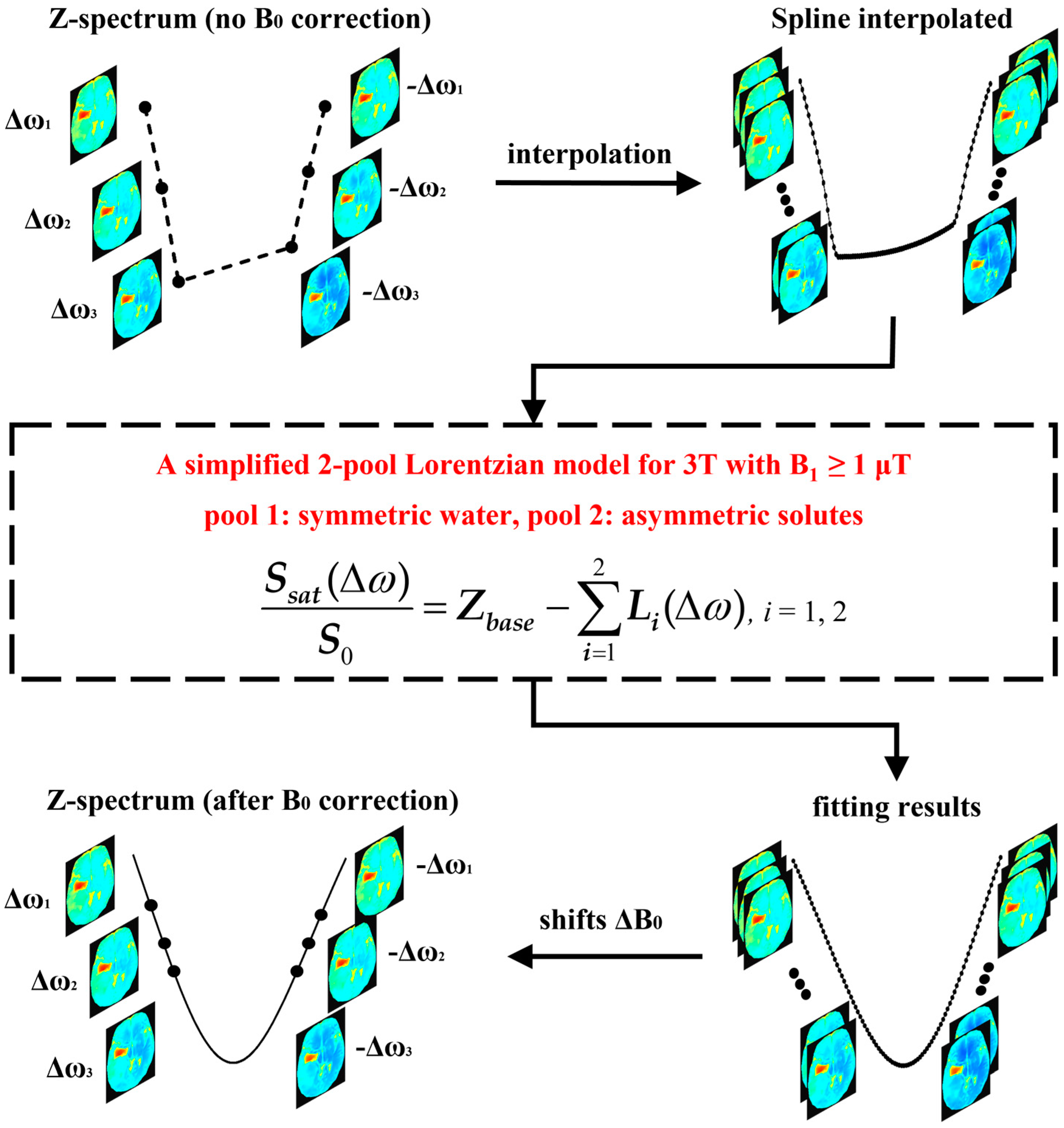
2. Theory
3. Materials and Methods
3.1. B0 inhomogeneity Correction
3.2. MTRasym Quantification of APT
3.3. Comparison Methods
3.4. Datasets
3.5. Evaluation Metrics
4. Results
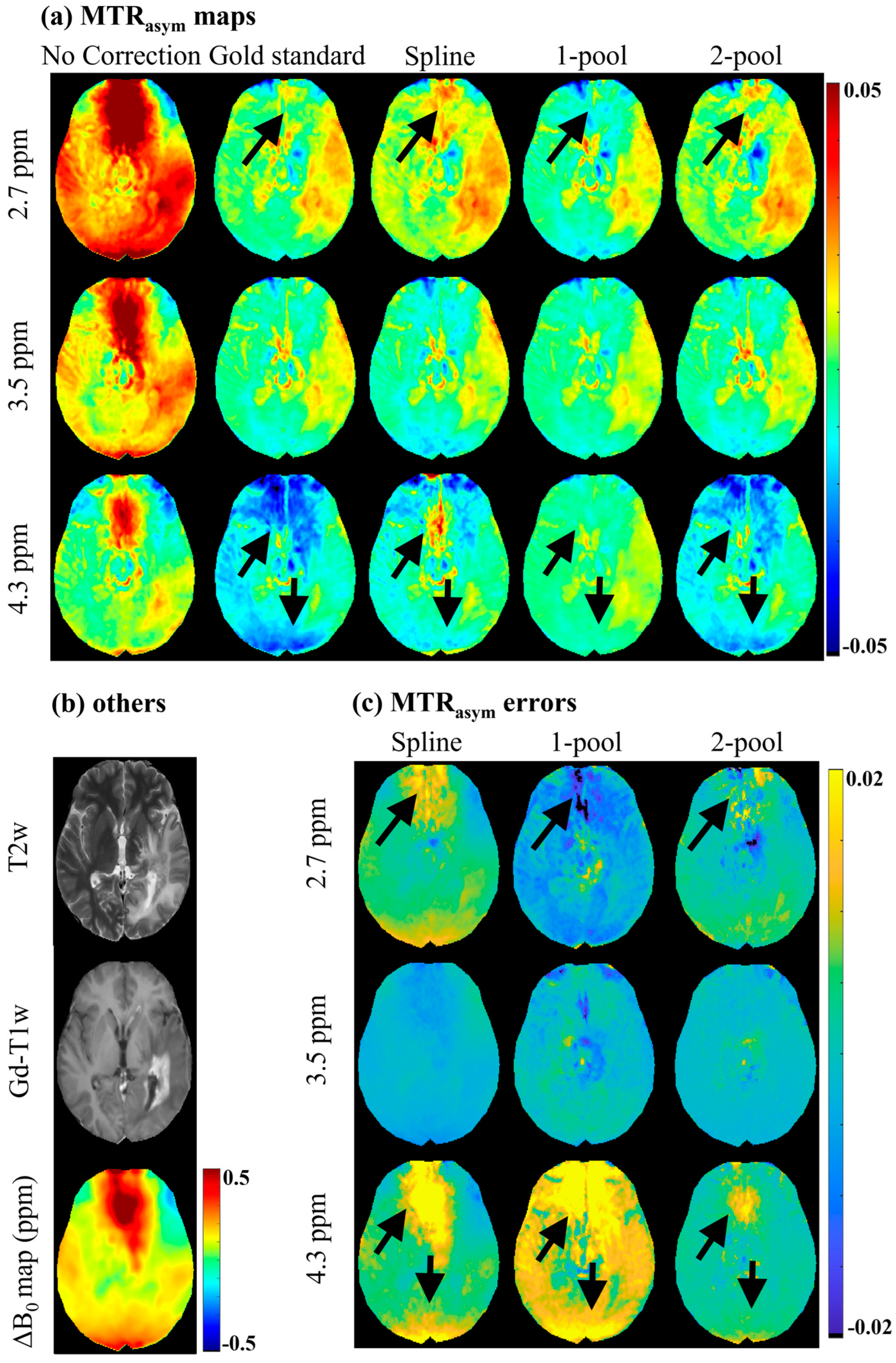
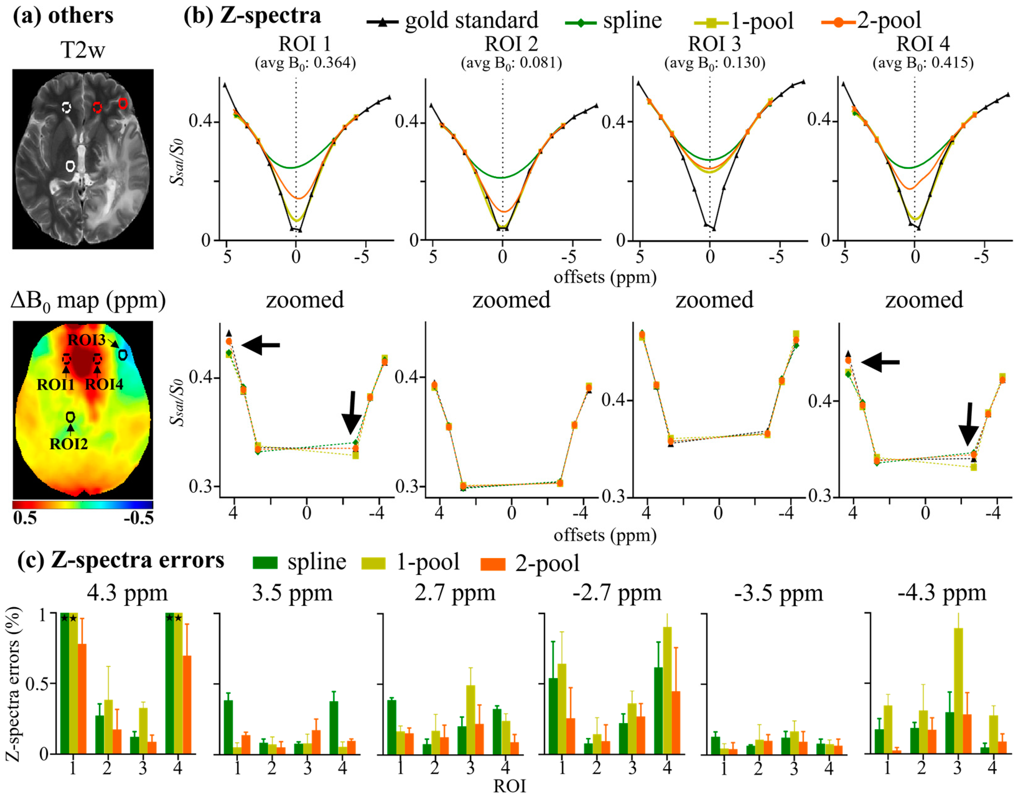
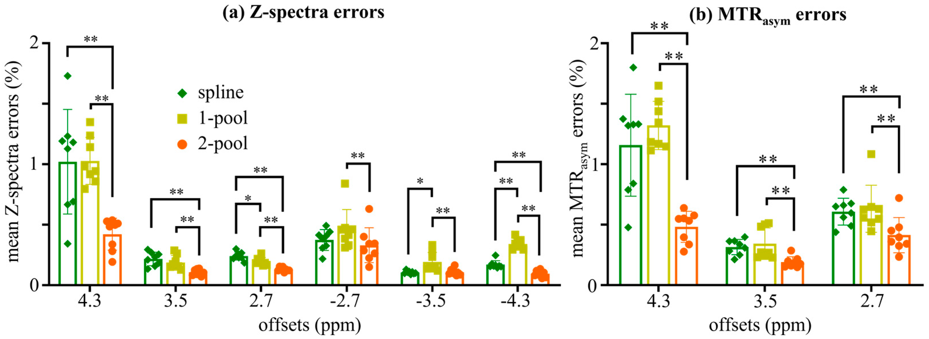
4.1. Accuracy Evaluation
4.2. Comparison with Vendor
5. Discussion
6. Conclusions
Supplementary Materials
Author Contributions
Funding
Institutional Review Board Statement
Informed Consent Statement
Data Availability Statement
Acknowledgments
Conflicts of Interest
Abbreviations
| APT | amide proton transfer |
| MTRasym | asymmetry analysis of magnetization transfer ratio |
| CEST | chemical exchange saturation transfer |
| ΔB0 | B0 inhomogeneity |
| WASSR | water saturation shift referencing |
| DS | direct water saturation |
| MT | magnetization transfer |
| NOE | nuclear Overhauser effect |
| Δi | central offset of the Lorentzian line |
| FWHM | peak full width at half maximum |
| Ai | peak amplitude |
| ROI | region-of-interest |
References
- Gao, T.; Zou, C.; Li, Y.; Jiang, Z.; Tang, X.; Song, X. A Brief History and Future Prospects of CEST MRI in Clinical Non-Brain Tumor Imaging. Int. J. Mol. Sci. 2021, 22, 1559. [Google Scholar] [CrossRef]
- Okuchi, S.; Hammam, A.; Golay, X.; Kim, M.; Thust, S. Endogenous Chemical Exchange Saturation Transfer MRI for the Diagnosis and Therapy Response Assessment of Brain Tumors: A Systematic Review. Radiol. Imaging Cancer 2020, 2, e190036. [Google Scholar] [CrossRef] [PubMed]
- Dou, W.; Lin, C.-Y.E.; Ding, H.; Shen, Y.; Dou, C.; Qian, L.; Wen, B.; Wu, B. Chemical exchange saturation transfer magnetic resonance imaging and its main and potential applications in pre-clinical and clinical studies. Quant. Imaging Med. Surg. 2019, 9, 1747–1766. [Google Scholar] [CrossRef]
- Zhou, J.Y.; Payen, J.F.; Wilson, D.A.; Traystman, R.J.; van Zijl, P.C.M. Using the amide proton signals of intracellular proteins and peptides to detect pH effects in MRI. Nat. Med. 2003, 9, 1085–1090. [Google Scholar] [CrossRef] [PubMed]
- Zhou, J.; Heo, H.-Y.; Knutsson, L.; van Zijl, P.C.M.; Jiang, S. APT-weighted MRI: Techniques, current neuro applications, and challenging issues. J. Magn. Reson. Imaging 2019, 50, 347–364. [Google Scholar] [CrossRef]
- Zhang, J.; Zhu, W.; Tain, R.; Zhou, X.J.; Cai, K. Improved Differentiation of Low-Grade and High-Grade Gliomas and Detection of Tumor Proliferation Using APT Contrast Fitted from Z-Spectrum. Mol. Imaging Biol. 2018, 20, 623–631. [Google Scholar] [CrossRef]
- Jiang, S.; Eberhart, C.G.; Lim, M.; Heo, H.Y.; Zhang, Y.; Blair, L.; Wen, Z.; Holdhoff, M.; Lin, D.; Huang, P.; et al. Identifying Recurrent Malignant Glioma after Treatment Using Amide Proton Transfer-Weighted MR Imaging: A Validation Study with Image-Guided Stereotactic Biopsy. Clin. Cancer Res. 2019, 25, 552–561. [Google Scholar] [CrossRef] [PubMed] [Green Version]
- Paech, D.; Dreher, C.; Regnery, S.; Meissner, J.E.; Goerke, S.; Windschuh, J.; Oberhollenzer, J.; Schultheiss, M.; Deike-Hofmann, K.; Bickelhaupt, S.; et al. Relaxation-compensated amide proton transfer (APT) MRI signal intensity is associated with survival and progression in high-grade glioma patients. Eur. Radiol. 2019, 29, 4957–4967. [Google Scholar] [CrossRef]
- Zhou, J.; Zaiss, M.; Knutsson, L.; Sun, P.Z.; Ahn, S.S.; Aime, S.; Bachert, P.; Blakeley, J.O.; Cai, K.; Chappell, M.A.; et al. Review and consensus recommendations on clinical APT-weighted imaging approaches at 3T: Application to brain tumors. Magn. Reson. Med. 2022, 88, 546–574. [Google Scholar] [CrossRef]
- Liu, R.; Zhang, H.; Niu, W.; Lai, C.; Ding, Q.; Chen, W.; Liang, S.; Zhou, J.; Wu, D.; Zhang, Y. Improved chemical exchange saturation transfer imaging with real-time frequency drift correction. Magn. Reson. Med. 2020, 83, 1884. [Google Scholar] [CrossRef]
- Simegn, G.L.; Van der Kouwe, A.J.W.; Robertson, F.C.; Meintjes, E.M.; Alhamud, A. Real-time simultaneous shim and motion measurement and correction in glycoCEST MRI using double volumetric navigators (DvNavs). Magn. Reson. Med. 2019, 81, 2600–2613. [Google Scholar] [CrossRef] [PubMed]
- Windschuh, J.; Zaiss, M.; Ehses, P.; Lee, J.-S.; Jerschow, A.; Regatte, R.R. Assessment of frequency drift on CEST MRI and dynamic correction: Application to gagCEST at 7 T. Magn. Reson. Med. 2019, 81, 573–582. [Google Scholar] [CrossRef] [PubMed]
- Poblador Rodriguez, E.; Moser, P.; Auno, S.; Eckstein, K.; Dymerska, B.; van der Kouwe, A.; Gruber, S.; Trattnig, S.; Bogner, W. Real-time motion and retrospective coil sensitivity correction for CEST using volumetric navigators (vNavs) at 7T. Magn. Reson. Med. 2021, 85, 1909–1923. [Google Scholar] [CrossRef]
- Yoo, C.H.; Oh, J.; Park, S.; Ryu, C.-W.; Kwon, Y.K.; Jahng, G.-H. Comparative evaluation of the polynomial and spline fitting methods for the B0 correction of CEST MRI data acquired from human brains. Int. J. Imaging Syst. Technol. 2019, 29, 272–282. [Google Scholar] [CrossRef]
- Debnath, A.; Gupta, R.K.; Reddy, R.; Singh, A. Effect of offset-frequency step size and interpolation methods on chemical exchange saturation transfer MRI computation in human brain. NMR Biomed. 2021, 34, e4468. [Google Scholar] [CrossRef] [PubMed]
- Sun, P.Z. Fast correction of B-0 field inhomogeneity for pH-specific magnetization transfer and relaxation normalized amide proton transfer imaging of acute ischemic stroke without Z-spectrum. Magn. Reson. Med. 2020, 83, 1688–1697. [Google Scholar] [CrossRef]
- Sun, P.Z.; Farrar, C.T.; Sorensen, A.G. Correction for artifacts induced by B-0 and B-1 field inhomogeneities in pH-Sensitive chemical exchange saturation transfer (CEST) Imaging. Magn. Reson. Med. 2007, 58, 1207–1215. [Google Scholar] [CrossRef]
- Li, Y.; Xie, D.; Cember, A.; Nanga, R.P.R.; Yang, H.; Kumar, D.; Hariharan, H.; Bai, L.; Detre, J.A.; Reddy, R.; et al. Accelerating GluCEST imaging using deep learning for B-0 correction. Magn. Reson. Med. 2020, 84, 1724–1733. [Google Scholar] [CrossRef]
- Kim, M.; Gillen, J.; Landman, B.A.; Zhou, J.; van Zijl, P.C.M. Water Saturation Shift Referencing (WASSR) for Chemical Exchange Saturation Transfer (CEST) Experiments. Magn. Reson. Med. 2009, 61, 1441–1450. [Google Scholar] [CrossRef] [Green Version]
- Mueller-Lutz, A.; Matuschke, F.; Schleich, C.; Wickrath, F.; Boos, J.; Schmitt, B.; Wittsack, H.-J. Improvement of water saturation shift referencing by sequence and analysis optimization to enhance chemical exchange saturation transfer imaging. Magn. Reson. Imaging 2016, 34, 771–778. [Google Scholar] [CrossRef]
- Togao, O.; Keupp, J.; Hiwatashi, A.; Yamashita, K.; Kikuchi, K.; Yoneyama, M.; Honda, H. Amide Proton Transfer Imaging of Brain Tumors Using a Self-Corrected 3D Fast Spin-Echo Dixon Method: Comparison With Separate B-0 Correction. Magn. Reson. Med. 2017, 77, 2272–2279. [Google Scholar] [CrossRef] [PubMed]
- Yao, J.; Ruan, D.; Raymond, C.; Liau, L.M.; Salamon, N.; Pope, W.B.; Nghiemphu, P.L.; Lai, A.; Cloughesy, T.F.; Ellingson, B.M. Improving B-0 Correction for pH-Weighted Amine Proton Chemical Exchange Saturation Transfer (CEST) Imaging by Use of k-Means Clustering and Lorentzian Estimation. Tomography 2018, 4, 123–137. [Google Scholar] [CrossRef]
- Lee, H.; Chung, J.J.; Lee, J.; Kim, S.G.; Han, J.H.; Park, J. Model-Based Chemical Exchange Saturation Transfer MRI for Robust z-Spectrum Analysis. IEEE Trans. Med. Imaging 2020, 39, 283–293. [Google Scholar] [CrossRef]
- Zhou, J.; Blakeley, J.O.; Hua, J.; Kim, M.; Laterra, J.; Pomper, M.G.; van Zijl, P.C. Practical data acquisition method for human brain tumor amide proton transfer (APT) imaging. Magn. Reson. Med. 2008, 60, 842–849. [Google Scholar] [CrossRef] [PubMed] [Green Version]
- Windschuh, J.; Zaiss, M.; Meissner, J.-E.; Paech, D.; Radbruch, A.; Ladd, M.E.; Bachert, P. Correction of B1-inhomogeneities for relaxation-compensated CEST imaging at 7T. NMR Biomed. 2015, 28, 529–537. [Google Scholar] [CrossRef]
- Cui, J.; Afzal, A.; Zu, Z. Comparative evaluation of polynomial and Lorentzian lineshape-fitted amine CEST imaging in acute ischemic stroke. Magn. Reson. Med. 2022, 87, 837–849. [Google Scholar] [CrossRef] [PubMed]
- Van de Ven, K.; Keupp, J. Amide proton transfer weighted imaging: Advancement in molecular tumor diagnosis. Philips White Pap. 2018. Available online: https://www.documents.philips.com/assets/20180614/1fa1f9ad18a74c2f9388a8ff008b3dcc.pdf (accessed on 30 June 2022).
- Stancanello, J.; Terreno, E.; Castelli, D.D.; Cabella, C.; Uggeri, F.; Aime, S. Development and validation of a smoothing-splines-based correction method for improving the analysis of CEST-MR images. Contrast Media Mol. Imaging 2008, 3, 136–149. [Google Scholar] [CrossRef]
- Goldenberg, J.M.; Pagel, M.D. Assessments of tumor metabolism with CEST MRI. NMR Biomed. 2019, 32, e3943. [Google Scholar] [CrossRef] [PubMed]
- Yelamanchi, S.D.; Jayaram, S.; Thomas, J.K.; Gundimeda, S.; Khan, A.A.; Singhal, A.; Keshava Prasad, T.S.; Pandey, A.; Somani, B.L.; Gowda, H. A pathway map of glutamate metabolism. J. Cell Commun. Signal 2016, 10, 69–75. [Google Scholar] [CrossRef] [Green Version]
- Cui, J.; Zu, Z. Towards the molecular origin of glutamate CEST (GluCEST) imaging in rat brain. Magn. Reson. Med. 2020, 83, 1405–1417. [Google Scholar] [CrossRef] [Green Version]
- Jia, Y.; Chen, Y.; Geng, K.; Cheng, Y.; Li, Y.; Qiu, J.; Huang, H.; Wang, R.; Zhang, Y.; Wu, R. Glutamate Chemical Exchange Saturation Transfer (GluCEST) Magnetic Resonance Imaging in Pre-clinical and Clinical Applications for Encephalitis. Front. NeuroSci. 2020, 14, 750. [Google Scholar] [CrossRef] [PubMed]
- Hilbert, T.; Xia, D.; Block, K.T.; Yu, Z.; Lattanzi, R.; Sodickson, D.K.; Kober, T.; Cloos, M.A. Magnetization transfer in magnetic resonance fingerprinting. Magn. Reson. Med. 2020, 84, 128–141. [Google Scholar] [CrossRef] [PubMed] [Green Version]
- Mehrabian, H.; Detsky, J.; Soliman, H.; Sahgal, A.; Stanisz, G.J. Advanced Magnetic Resonance Imaging Techniques in Management of Brain Metastases. Front. Oncol. 2019, 9, 440. [Google Scholar] [CrossRef] [PubMed]
- Mehrabian, H.; Myrehaug, S.; Soliman, H.; Sahgal, A.; Stanisz, G.J. Quantitative Magnetization Transfer in Monitoring Glioblastoma (GBM) Response to Therapy. Sci. Rep. 2018, 8, 2475. [Google Scholar] [CrossRef] [PubMed] [Green Version]
- Chen, Y.; Dang, X.; Zhao, B.; Chen, Z.; Zhao, Y.; Zhao, F.; Zheng, Z.; He, X.; Peng, J.; Song, X. Frequency importance analysis for chemical exchange saturation transfer magnetic resonance imaging using permuted random forest. NMR Biomed. 2022, 18, e4744. [Google Scholar] [CrossRef] [PubMed]
- Zaiss, M.; Deshmane, A.; Schuppert, M.; Herz, K.; Glang, F.; Ehses, P.; Lindig, T.; Bender, B.; Ernemann, U.; Scheffler, K. DeepCEST: 9.4 T Chemical exchange saturation transfer MRI contrast predicted from 3 T data—A proof of concept study. Magn. Reson. Med. 2019, 81, 3901–3914. [Google Scholar] [CrossRef] [Green Version]

| Δ1 | W1 | A1 | Δ2 | W2 | A2 | Zbase | |
|---|---|---|---|---|---|---|---|
| start | 0 | 50 | 25 | −2 | 50 | 0.1 | 0.7 |
| lower | −0.5 | 0 | 0 | −4 | −inf | −inf | −inf |
| upper | 0.5 | 100 | 50 | 4 | +inf | +inf | +inf |
Publisher’s Note: MDPI stays neutral with regard to jurisdictional claims in published maps and institutional affiliations. |
© 2022 by the authors. Licensee MDPI, Basel, Switzerland. This article is an open access article distributed under the terms and conditions of the Creative Commons Attribution (CC BY) license (https://creativecommons.org/licenses/by/4.0/).
Share and Cite
Chen, Y.; Dang, X.; Zhao, B.; Zheng, Z.; He, X.; Song, X. B0 Correction for 3T Amide Proton Transfer (APT) MRI Using a Simplified Two-Pool Lorentzian Model of Symmetric Water and Asymmetric Solutes. Tomography 2022, 8, 1974-1986. https://doi.org/10.3390/tomography8040165
Chen Y, Dang X, Zhao B, Zheng Z, He X, Song X. B0 Correction for 3T Amide Proton Transfer (APT) MRI Using a Simplified Two-Pool Lorentzian Model of Symmetric Water and Asymmetric Solutes. Tomography. 2022; 8(4):1974-1986. https://doi.org/10.3390/tomography8040165
Chicago/Turabian StyleChen, Yibing, Xujian Dang, Benqi Zhao, Zhuozhao Zheng, Xiaowei He, and Xiaolei Song. 2022. "B0 Correction for 3T Amide Proton Transfer (APT) MRI Using a Simplified Two-Pool Lorentzian Model of Symmetric Water and Asymmetric Solutes" Tomography 8, no. 4: 1974-1986. https://doi.org/10.3390/tomography8040165
APA StyleChen, Y., Dang, X., Zhao, B., Zheng, Z., He, X., & Song, X. (2022). B0 Correction for 3T Amide Proton Transfer (APT) MRI Using a Simplified Two-Pool Lorentzian Model of Symmetric Water and Asymmetric Solutes. Tomography, 8(4), 1974-1986. https://doi.org/10.3390/tomography8040165