


Multi-Strategy Improved Sand Cat Swarm Optimization: Global Optimization and Feature Selection


Abstract
:1. Introduction
- ♦
- Three improvement strategies (novel opposition-based learning strategy, novel exploration mechanism, and biological elimination update mechanism) are used to improve the optimization performance of the SCSO algorithm.
- ♦
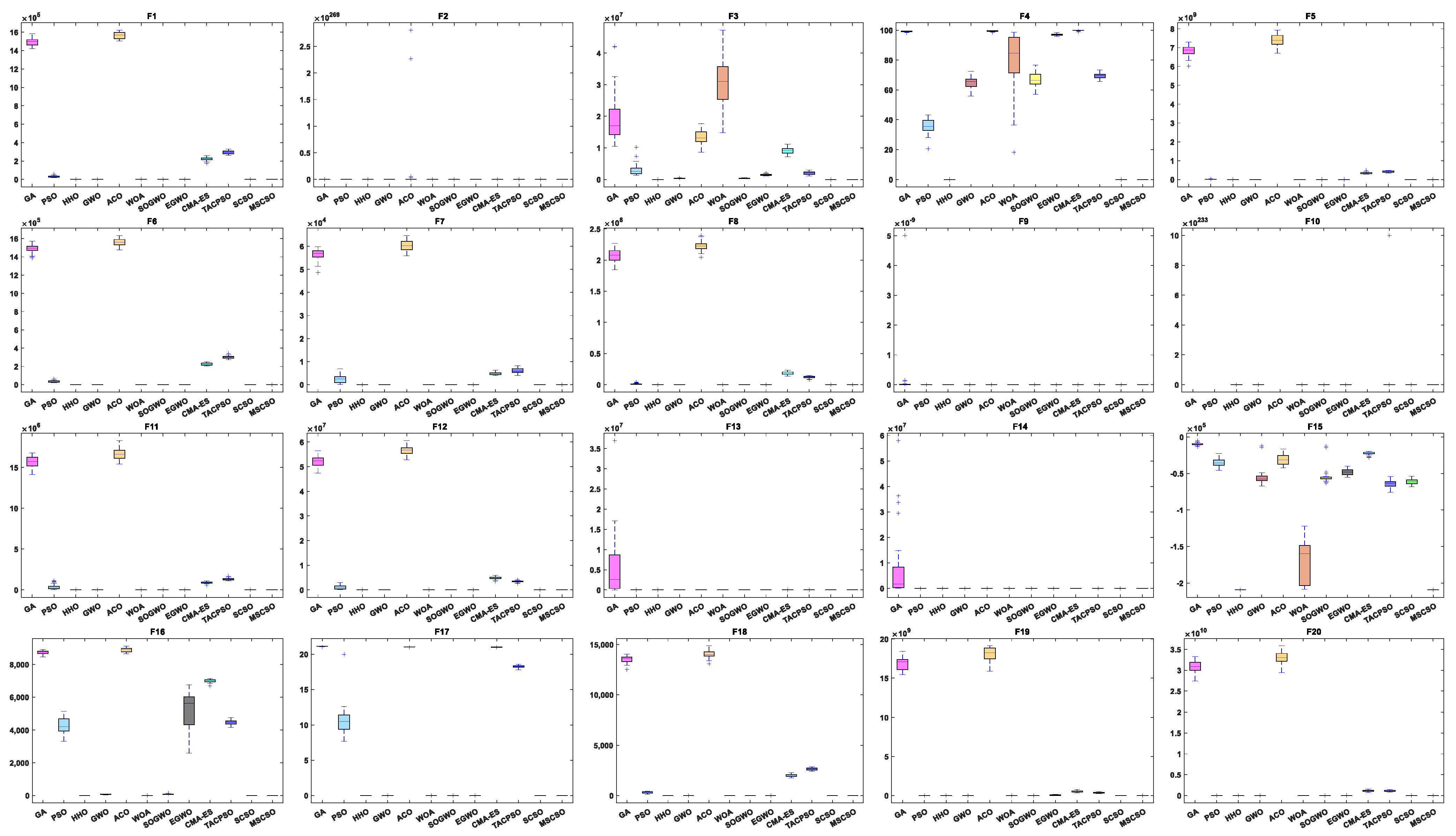
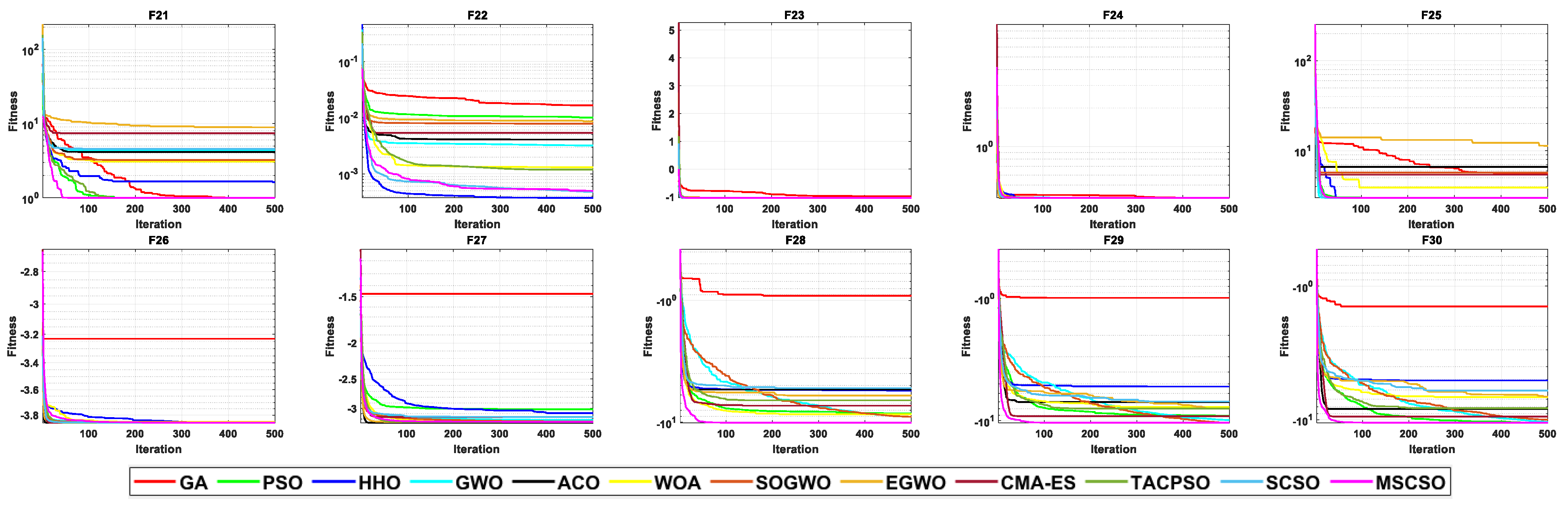
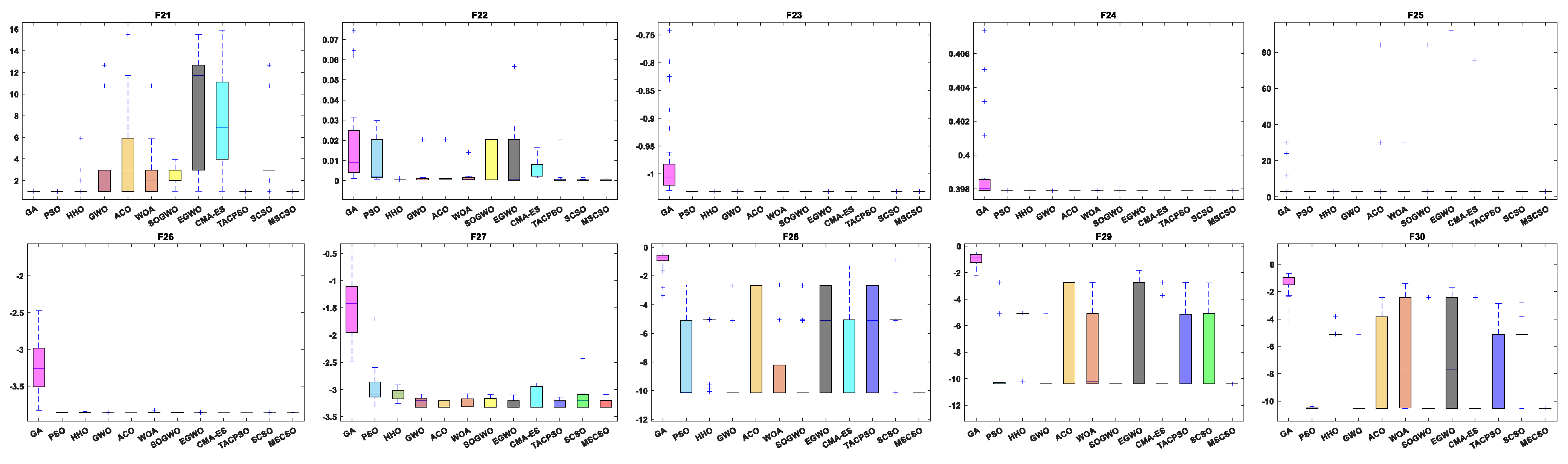
- Thirty standard test functions for intelligent optimization algorithm testing are used to evaluate the proposed MSCSO and compare the results with 11 other advanced optimization algorithms.
- ♦
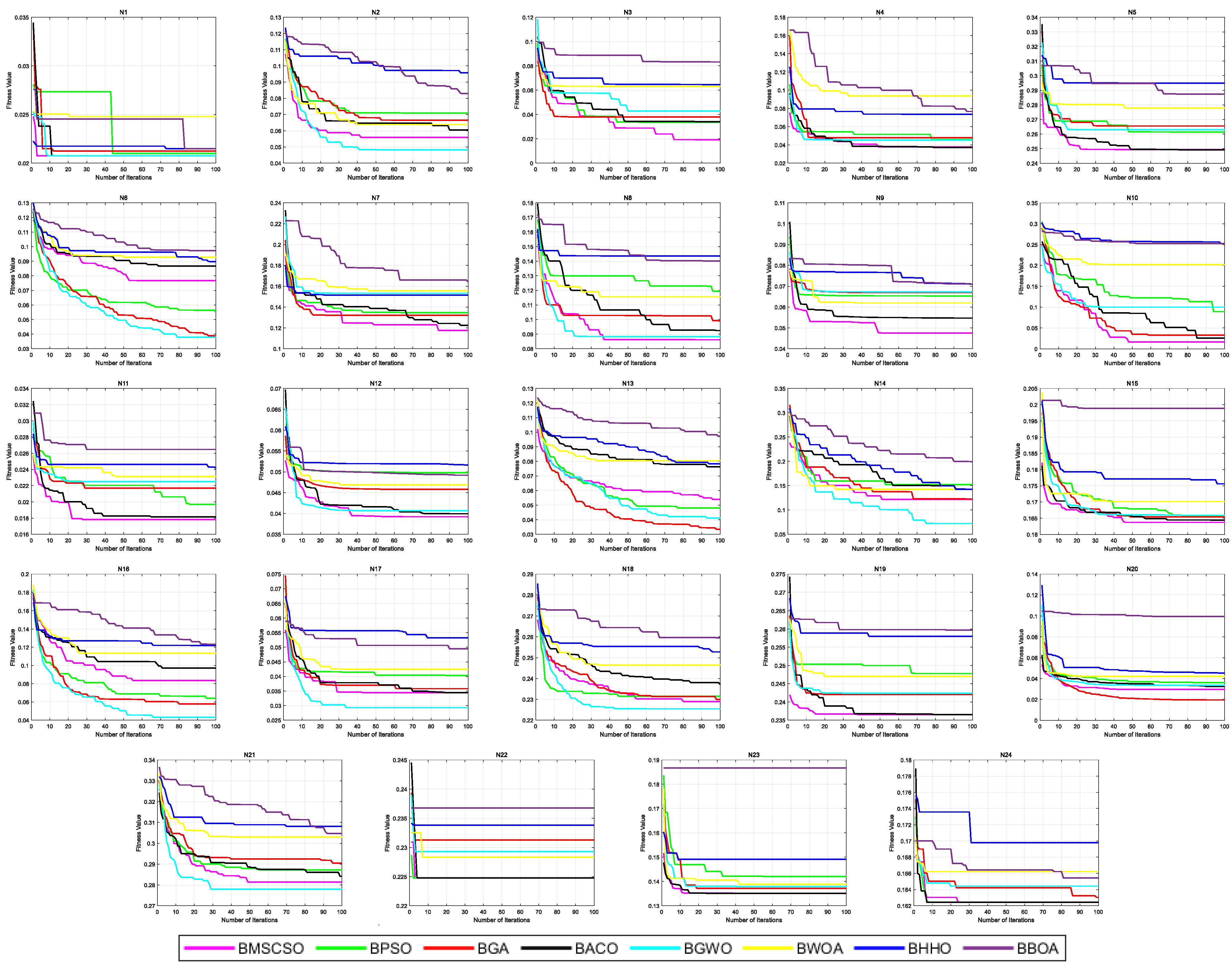
- Twenty-four feature selection datasets were used to evaluate the proposed MSCSO and compare the results with other advanced optimization algorithms.
2. Original SCSO
| Algorithm 1 The pseudocode of the SCSO | |
| 1. | Initialize the population Si |
| 2. | Calculate the fitness function based on the objective function |
| 3. | Initialize the |
| 4. | While (t < = ) |
| 5. | For each search agent |
| 6. | Obtain a random angle based on the Roulette Wheel Selection () |
| 7. | If (abs(R) > 1) |
| 8. | Update the search agent position based on the Equation (6) |
| 9. | Else |
| 10. | Update the search agent position based on the Equation (8) |
| 11 | End |
| 12. | End |
| 13. | t = t + 1 |
| 14. | End |
3. Proposed MSCSO
3.1. Nonlinear Lens Imaging Strategy
3.2. Novel Exploration Mechanisms
3.3. Elimination and Update Mechanism
| Algorithm 2. The pseudocode of MSCSO. | |
| 1. | Initialize the population |
| 2. | Calculate the fitness function based on the objective function |
| 3. | Initialize the |
| 4. | While (t <= ) |
| 5. | For each search agent |
| 6. | Obtain a random angle based on the Roulette Wheel Selection () |
| 7 | Obtain new position by Equation (10) |
| 8 | Calculate the fitness function values to obtain the optimal position |
| 9. | If (abs(R) > 1) |
| 10. | Update the search agent position based on the Equation (12) |
| 11. | Else |
| 12. | Update the search agent position based on the Equation (8) |
| 13 | End |
| 14 | Update new position using Equation (13) |
| 15 | Check the boundaries of new position and calculate fitness value |
| 16. | End |
| 17 | Find the current best solution |
| 18. | t = t + 1 |
| 19. | End |
3.4. Time Complexity of MSCSO
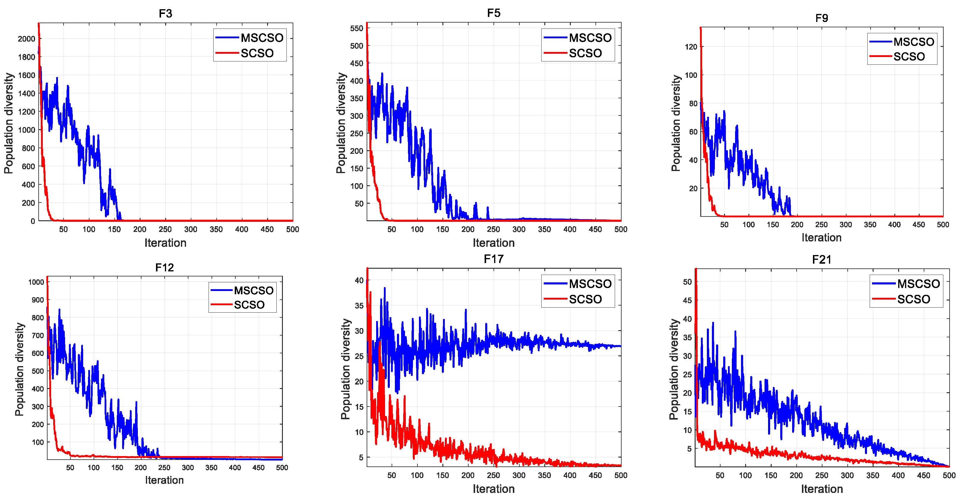
3.5. Population Diversity of MSCSO
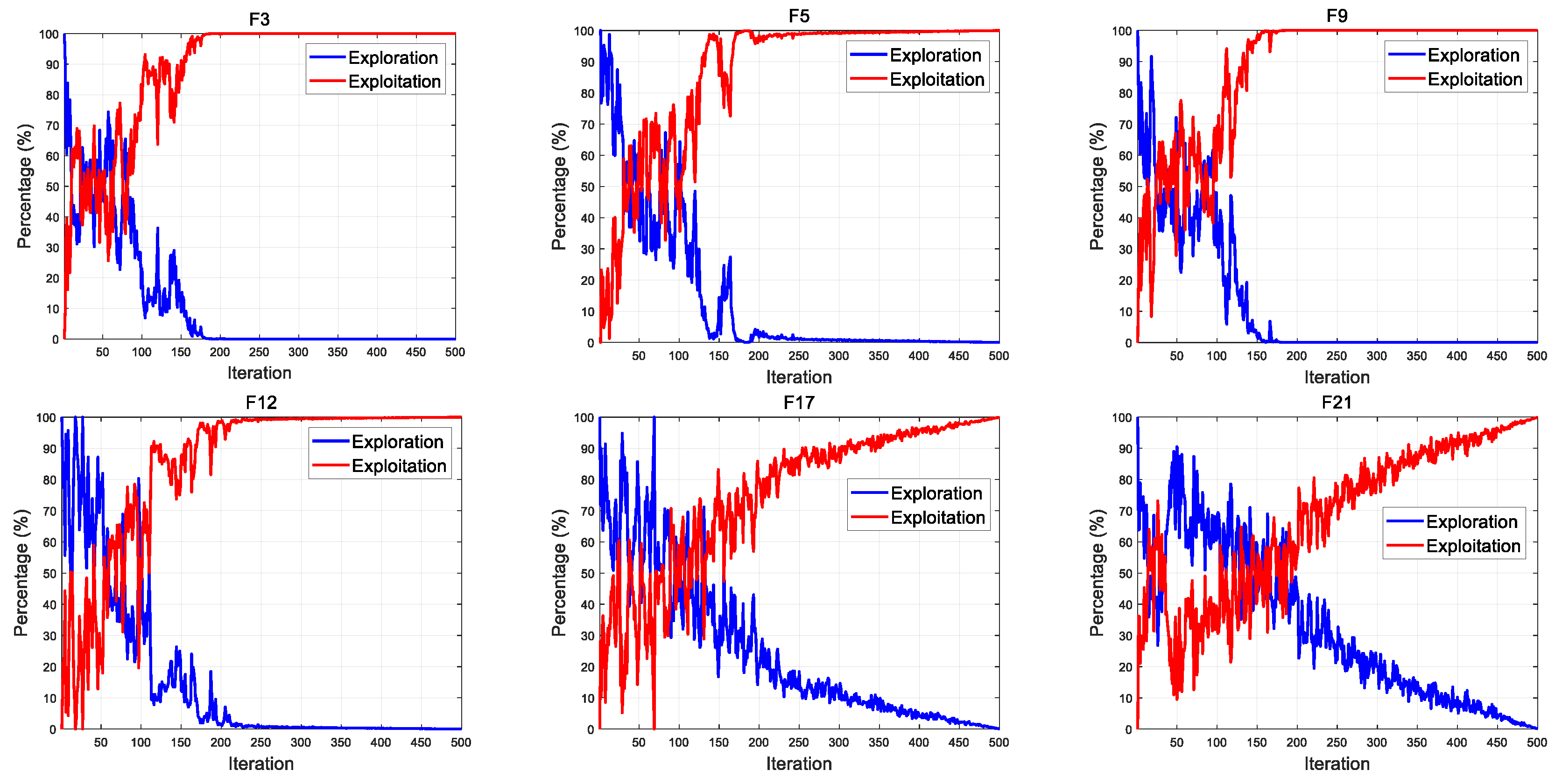
3.6. Exploration and Exploitation of MSCSO
4. Experiments and Results Analysis
4.1. Benchmark Datasets
4.2. Parameter Settings
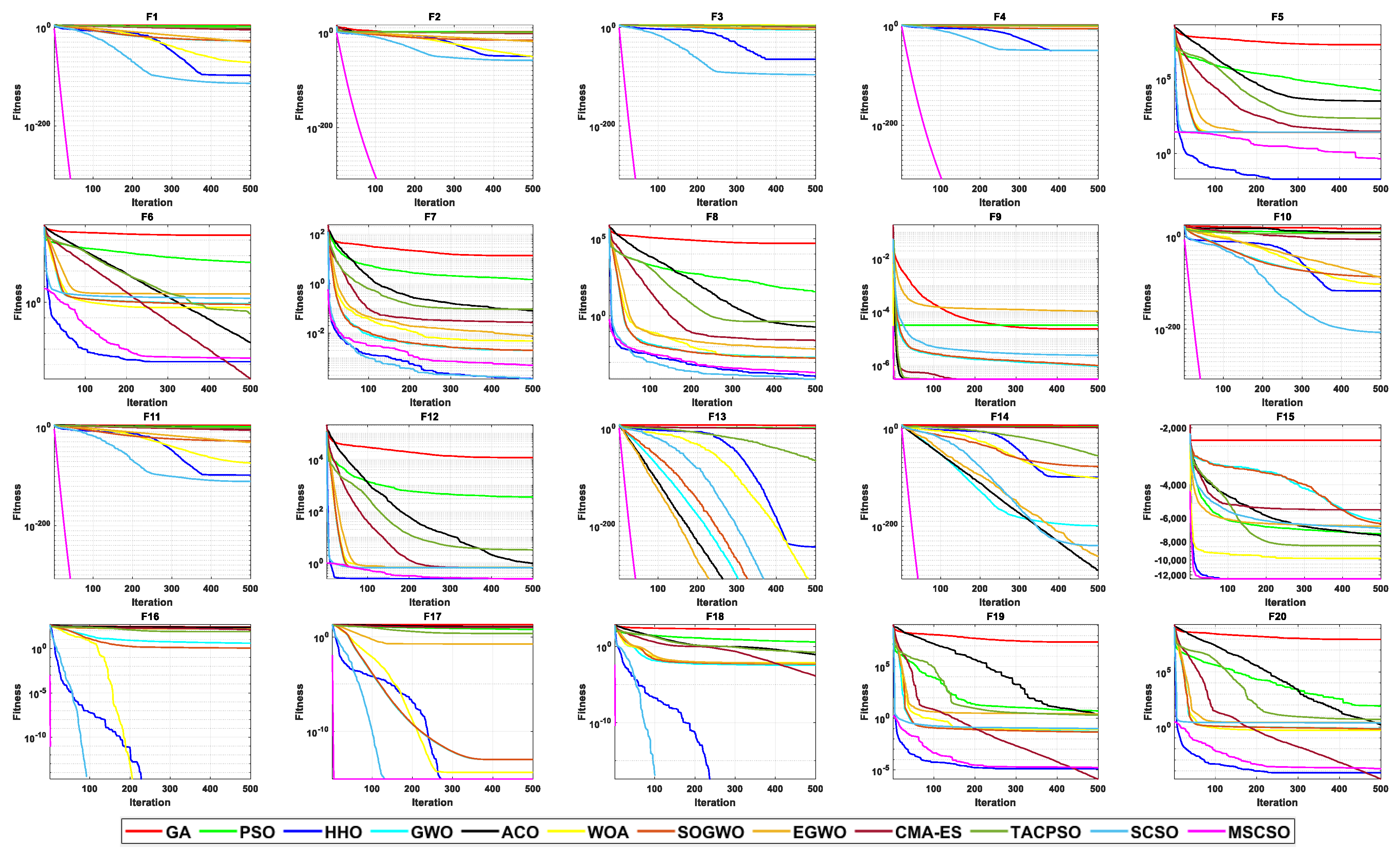
4.3. Results Analysis
5. Conclusions and Future Works
Author Contributions
Funding
Institutional Review Board Statement
Informed Consent Statement
Data Availability Statement
Conflicts of Interest
Appendix A

| Name | Function | Dim | Range | Type | |
|---|---|---|---|---|---|
| Sphere | 30, 100, 500 | [−100, 100] | 0 | Unimodal | |
| Schwefel 2.22 | 30, 100, 500 | [−1.28, 1.28] | 0 | Unimodal | |
| Schwefel 1.2 | 30, 100, 500 | [−100, 100] | 0 | Unimodal | |
| Schwefel 2.21 | 30, 100, 500 | [−100, 100] | 0 | Unimodal | |
| Rosenbroke | 30, 100, 500 | [−30, 30] | 0 | Unimodal | |
| Step | 30, 100, 500 | [−100, 100] | 0 | Unimodal | |
| Quartic | 30, 100, 500 | [−1.28, 1.28] | 0 | Unimodal | |
| Exponential | 30, 100, 500 | [−10, 10] | 0 | Unimodal | |
| Sum Power | 30, 100, 500 | [−1, 1] | 0 | Unimodal | |
| Sum Square | 30, 100, 500 | [−10, 10] | 0 | Unimodal | |
| Zakharov | 30, 100, 500 | [−10, 10] | 0 | Unimodal | |
| Trid | 30, 100, 500 | [−10, 10] | 0 | Unimodal | |
| Elliptic | 30, 100, 500 | [−100, 100] | 0 | Unimodal | |
| Cigar | 30, 100, 500 | [−100, 100] | 0 | Unimodal | |
| Generalized Schwefel’s problem 2.26 | 30, 100, 500 | [−500, 500] | −418.9829 × n | Multimodal | |
| Generalized Rastrigin’s Function | 30, 100, 500 | [−5.12, 5.12] | 0 | Multimodal | |
| Ackley’s Function | 30, 100, 500 | [−32, 32] | 0 | Multimodal | |
| Generalized Criewank Function | 30, 100, 500 | [−600, 600] | 0 | Multimodal | |
| Penalized 1 | 30, 100, 500 | [−50, 50] | 0 | Multimodal | |
| Penalized 2 | 30, 100, 500 | [−50, 50] | 0 | Multimodal | |
| Shekell’s Foxholes Function | 2 | [−65.536, 65.536] | 1 | Multimodal | |
| Kowalik’s Function | 4 | [−5, 5] | 0.0003 | Multimodal | |
| Six-Hump Camel-Back Function | 2 | [−5, 5] | −1.0316 | Multimodal | |
| Branin Function | 2 | [−5, 5] | 0.398 | Multimodal | |
| Goldstein-Price Function | 2 | [−2, 2] | 3 | Multimodal | |
| Hatman’s Function1 | 3 | [0, 1] | −3.86 | Multimodal | |
| Hatman’s Function2 | 6 | [0, 1] | −3.32 | Multimodal | |
| Schekel’s Family 1 | 4 | [0, 10] | −10.1532 | Multimodal | |
| Schekel’s Family 2 | 4 | [0, 10] | −10.4028 | Multimodal | |
| Schekel’s Family 3 | 4 | [0, 10] | −10.5364 | Multimodal |
References
- Yuan, Y.; Wei, J.; Huang, H.; Jiao, W.; Wang, J.; Chen, H. Review of resampling techniques for the treatment of imbalanced industrial data classification in equipment condition monitoring. Eng. Appl. Artif. Intell. 2023, 126, 106911. [Google Scholar] [CrossRef]
- Liang, Y.-C.; Minanda, V.; Gunawan, A. Waste collection routing problem: A mini-review of recent heuristic approaches and applications. Waste Manag. Res. 2022, 40, 519–537. [Google Scholar] [CrossRef] [PubMed]
- Kuo, R.; Li, S.-S. Applying particle swarm optimization algorithm-based collaborative filtering recommender system considering rating and review. Appl. Soft Comput. 2023, 135, 110038. [Google Scholar] [CrossRef]
- Fan, S.-K.S.; Lin, W.-K.; Jen, C.-H. Data-driven optimization of accessory combinations for final testing processes in semiconductor manufacturing. J. Manuf. Syst. 2022, 63, 275–287. [Google Scholar] [CrossRef]
- Huynh, N.-T.; Nguyen, T.V.T.; Tam, N.T.T.; Nguyen, Q. Optimizing Magnification Ratio for the Flexible Hinge Displacement Amplifier Mechanism Design. In Lecture Notes in Mechanical Engineering, Proceedings of the 2nd Annual International Conference on Material, Machines and Methods for Sustainable Development (MMMS2020), Nha Trang, Vietnam, 12–15 November 2020; Springer: Cham, Switzerland, 2021. [Google Scholar]
- Kler, R.; Gangurde, R.; Elmirzaev, S.; Hossain, M.S.; Vo, N.T.M.; Nguyen, T.V.T.; Kumar, P.N. Optimization of Meat and Poultry Farm Inventory Stock Using Data Analytics for Green Supply Chain Network. Discret. Dyn. Nat. Soc. 2022, 2022, 8970549. [Google Scholar] [CrossRef]
- Yu, K.; Liang, J.J.; Qu, B.; Luo, Y.; Yue, C. Dynamic Selection Preference-Assisted Constrained Multiobjective Differential Evolution. IEEE Trans. Syst. Man Cybern. Syst. 2021, 52, 2954–2965. [Google Scholar] [CrossRef]
- Yu, K.; Sun, S.; Liang, J.J.; Chen, K.; Qu, B.; Yue, C.; Wang, L. A bidirectional dynamic grouping multi-objective evolutionary algorithm for feature selection on high-dimensional classification. Inf. Sci. 2023, 648, 119619. [Google Scholar] [CrossRef]
- Tang, J.; Liu, G.; Pan, Q. A review on representative swarm intelligence algorithms for solving optimization problems: Applications and trends. IEEE/CAA J. Autom. Sin. 2021, 8, 1627–1643. [Google Scholar] [CrossRef]
- Yu, K.; Zhang, D.; Liang, J.J.; Chen, K.; Yue, C.; Qiao, K.; Wang, L. A Correlation-Guided Layered Prediction Approach for Evolutionary Dynamic Multiobjective Optimization. IEEE Trans. Evol. Comput. 2023, 27, 1398–1412. [Google Scholar] [CrossRef]
- Wei, J.; Huang, H.; Yao, L.; Hu, Y.; Fan, Q.; Huang, D. New imbalanced bearing fault diagnosis method based on Sample-characteristic Oversampling TechniquE (SCOTE) and multi-class LS-SVM. Appl. Soft Comput. 2021, 101, 107043. [Google Scholar] [CrossRef]
- Yu, K.; Zhang, D.; Liang, J.J.; Qu, B.; Liu, M.; Chen, K.; Yue, C.; Wang, L. A Framework Based on Historical Evolution Learning for Dynamic Multiobjective Optimization. IEEE Trans. Evol. Comput. 2023. early access. [Google Scholar] [CrossRef]
- Seyyedabbasi, A.; Kiani, F. Sand Cat swarm optimization: A nature-inspired algorithm to solve global optimization problems. Eng. Comput. 2023, 39, 2627–2651. [Google Scholar] [CrossRef]
- Chu, S.-C.; Tsai, P.-W.; Pan, J.-S. Cat swarm optimization. In PRICAI 2006: Trends in Artificial Intelligence, Proceedings of the 9th Pacific Rim International Conference on Artificial Intelligence, Guilin, China, 7–11 August 2006; Proceedings 9; Springer: Cham, Switzerland, 2006; pp. 854–858. [Google Scholar]
- Mirjalili, S.; Mirjalili, S.M.; Lewis, A. Grey wolf optimizer. Adv. Eng. Softw. 2014, 69, 46–61. [Google Scholar] [CrossRef]
- Mirjalili, S.; Lewis, A. The whale optimization algorithm. Adv. Eng. Softw. 2016, 95, 51–67. [Google Scholar] [CrossRef]
- Mirjalili, S.; Gandomi, A.H.; Mirjalili, S.Z.; Saremi, S.; Faris, H.; Mirjalili, S.M. Salp Swarm Algorithm: A bio-inspired optimizer for engineering design problems. Adv. Eng. Softw. 2017, 114, 163–191. [Google Scholar] [CrossRef]
- Rashedi, E.; Nezamabadi-Pour, H.; Saryazdi, S. GSA: A gravitational search algorithm. Inf. Sci. 2009, 179, 2232–2248. [Google Scholar] [CrossRef]
- Kennedy, J.; Eberhart, R. Particle swarm optimization. In Proceedings of the ICNN’95—International Conference on Neural Networks, Perth, Australia, 27 November–1 December 1995; pp. 1942–1948. [Google Scholar]
- Hayyolalam, V.; Kazem, A.A.P. Black widow optimization algorithm: A novel meta-heuristic approach for solving engineering optimization problems. Eng. Appl. Artif. Intell. 2020, 87, 103249. [Google Scholar] [CrossRef]
- Hu, G.; Guo, Y.; Wei, G.; Abualigah, L. Genghis Khan shark optimizer: A novel nature-inspired algorithm for engineering optimization. Adv. Eng. Inform. 2023, 58, 102210. [Google Scholar] [CrossRef]
- Heidari, A.A.; Mirjalili, S.; Faris, H.; Aljarah, I.; Mafarja, M.; Chen, H. Harris hawks optimization: Algorithm and applications. Future Gener. Comput. Syst. 2019, 97, 849–872. [Google Scholar] [CrossRef]
- Hashim, F.A.; Hussien, A.G. Snake Optimizer: A novel meta-heuristic optimization algorithm. Knowl.-Based Syst. 2022, 242, 108320. [Google Scholar] [CrossRef]
- Xue, J.; Shen, B. Dung beetle optimizer: A new meta-heuristic algorithm for global optimization. J. Supercomput. 2023, 79, 7305–7336. [Google Scholar] [CrossRef]
- Jia, H.; Rao, H.; Wen, C.; Mirjalili, S. Crayfish optimization algorithm. Artif. Intell. Rev. 2023, 1–61. [Google Scholar] [CrossRef]
- Wei, J.; Wang, J.; Huang, H.; Jiao, W.; Yuan, Y.; Chen, H.; Wu, R.; Yi, J. Novel extended NI-MWMOTE-based fault diagnosis method for data-limited and noise-imbalanced scenarios. Expert Syst. Appl. 2023, 238, 121799. [Google Scholar] [CrossRef]
- Kiani, F.; Nematzadeh, S.; Anka, F.A.; Fındıklı, M. Chaotic Sand Cat Swarm Optimization. Mathematics 2023, 11, 2340. [Google Scholar] [CrossRef]
- Seyyedabbasi, A. Binary Sand Cat Swarm Optimization Algorithm for Wrapper Feature Selection on Biological Data. Biomimetics 2023, 8, 310. [Google Scholar] [CrossRef] [PubMed]
- Qtaish, A.; Albashish, D.; Braik, M.; Alshammari, M.T.; Alreshidi, A.; Alreshidi, E. Memory-Based Sand Cat Swarm Optimization for Feature Selection in Medical Diagnosis. Electronics 2023, 12, 2042. [Google Scholar] [CrossRef]
- Wu, D.; Rao, H.; Wen, C.; Jia, H.; Liu, Q.; Abualigah, L. Modified Sand Cat Swarm Optimization Algorithm for Solving Constrained Engineering Optimization Problems. Mathematics 2022, 10, 4350. [Google Scholar] [CrossRef]
- Kiani, F.; Anka, F.A.; Erenel, F. PSCSO: Enhanced sand cat swarm optimization inspired by the political system to solve complex problems. Adv. Eng. Softw. 2023, 178, 103423. [Google Scholar] [CrossRef]
- Yao, L.; Yuan, P.; Tsai, C.-Y.; Zhang, T.; Lu, Y.; Ding, S. ESO: An Enhanced Snake Optimizer for Real-world Engineering Problems. Expert Syst. Appl. 2023, 230, 120594. [Google Scholar] [CrossRef]
- Yuan, P.; Zhang, T.; Yao, L.; Lu, Y.; Zhuang, W. A Hybrid Golden Jackal Optimization and Golden Sine Algorithm with Dynamic Lens-Imaging Learning for Global Optimization Problems. Appl. Sci. 2022, 12, 9709. [Google Scholar] [CrossRef]
- Yao, L.; Li, G.; Yuan, P.; Yang, J.; Tian, D.; Zhang, T. Reptile Search Algorithm Considering Different Flight Heights to Solve Engineering Optimization Design Problems. Biomimetics 2023, 8, 305. [Google Scholar] [CrossRef] [PubMed]
- Zhong, C.; Li, G.; Meng, Z. Beluga whale optimization: A novel nature-inspired metaheuristic algorithm. Knowl.-Based Syst. 2022, 251, 109215. [Google Scholar] [CrossRef]
- Abed-Alguni, B.H.; Alawad, N.A.; Al-Betar, M.A.; Paul, D. Opposition-based sine cosine optimizer utilizing refraction learning and variable neighborhood search for feature selection. Appl. Intell. 2023, 53, 13224–13260. [Google Scholar] [CrossRef] [PubMed]
- Ma, C.; Huang, H.; Fan, Q.; Wei, J.; Du, Y.; Gao, W. Grey wolf optimizer based on Aquila exploration method. Expert Syst. Appl. 2022, 205, 117629. [Google Scholar] [CrossRef]
- Wu, R.; Huang, H.; Wei, J.; Ma, C.; Zhu, Y.; Chen, Y.; Fan, Q. An improved sparrow search algorithm based on quantum computations and multi-strategy enhancement. Expert Syst. Appl. 2022, 215, 119421. [Google Scholar] [CrossRef]
- Fan, Q.; Huang, H.; Chen, Q.; Yao, L.; Yang, K.; Huang, D. A modified self-adaptive marine predators algorithm: Framework and engineering applications. Eng. Comput. 2021, 38, 3269–3294. [Google Scholar] [CrossRef]
- Wang, Y.; Ran, S.; Wang, G.-G. Role-Oriented Binary Grey Wolf Optimizer Using Foraging-Following and Lévy Flight for Feature Selection. Appl. Math. Model. 2023, in press. [CrossRef]
- Lahmar, I.; Zaier, A.; Yahia, M.; Boaullègue, R. A Novel Improved Binary Harris Hawks Optimization For High dimensionality Feature Selection. Pattern Recognit. Lett. 2023, 171, 170–176. [Google Scholar] [CrossRef]
- Turkoglu, B.; Uymaz, S.A.; Kaya, E. Binary Artificial Algae Algorithm for feature selection. Appl. Soft Comput. 2022, 120, 108630. [Google Scholar] [CrossRef]
- Hu, G.; Zhong, J.; Zhao, C.; Wei, G.; Chang, C.-T. LCAHA: A hybrid artificial hummingbird algorithm with multi-strategy for engineering applications. Comput. Methods Appl. Mech. Eng. 2023, 415, 116238. [Google Scholar] [CrossRef]
- Long, W.; Jiao, J.; Xu, M.; Tang, M.; Wu, T.; Cai, S. Lens-imaging learning Harris hawks optimizer for global optimization and its application to feature selection. Expert Syst. Appl. 2022, 202, 117255. [Google Scholar] [CrossRef]
- Chen, H.; Xu, Y.; Wang, M.; Zhao, X. A balanced whale optimization algorithm for constrained engineering design problems. Appl. Math. Model. 2019, 71, 45–59. [Google Scholar] [CrossRef]
- Jia, H.; Li, Y.; Wu, D.; Rao, H.; Wen, C.; Abualigah, L. Multi-strategy Remora Optimization Algorithm for Solving Multi-extremum Problems. J. Comput. Des. Eng. 2023, 10, qwad044. [Google Scholar] [CrossRef]
- Nadimi-Shahraki, M.H.; Zamani, H. DMDE: Diversity-maintained multi-trial vector differential evolution algorithm for non-decomposition large-scale global optimization. Expert Syst. Appl. 2022, 198, 116895. [Google Scholar] [CrossRef]
- Holland, J.H. Genetic algorithms. Sci. Am. 1992, 267, 66–73. [Google Scholar] [CrossRef]
- Dorigo, M.; Birattari, M.; Stutzle, T. Ant colony optimization. IEEE Comput. Intell. Mag. 2006, 1, 28–39. [Google Scholar] [CrossRef]
- Dhargupta, S.; Ghosh, M.; Mirjalili, S.; Sarkar, R. Selective opposition based grey wolf optimization. Expert Syst. Appl. 2020, 151, 113389. [Google Scholar] [CrossRef]
- Komathi, C.; Umamaheswari, M. Design of gray wolf optimizer algorithm-based fractional order PI controller for power factor correction in SMPS applications. IEEE Trans. Power Electron. 2019, 35, 2100–2118. [Google Scholar] [CrossRef]
- Ziyu, T.; Dingxue, Z. A modified particle swarm optimization with an adaptive acceleration coefficients. In Proceedings of the 2009 Asia-Pacific Conference on Information Processing, Shenzhen, China, 18–19 July 2009; pp. 330–332. [Google Scholar]
- Ewees, A.A.; Ismail, F.H.; Sahlol, A.T. Gradient-based optimizer improved by Slime Mould Algorithm for global optimization and feature selection for diverse computation problems. Expert Syst. Appl. 2023, 213, 118872. [Google Scholar] [CrossRef]
- Sun, L.; Si, S.; Zhao, J.; Xu, J.; Lin, Y.; Lv, Z. Feature selection using binary monarch butterfly optimization. Appl. Intell. 2023, 53, 706–727. [Google Scholar] [CrossRef]

| No. | Datasets | Features | Samples | No. | Datasets | Features | Samples |
|---|---|---|---|---|---|---|---|
| 1 | Iris | 4 | 150 | 13 | Clean1 | 167 | 476 |
| 2 | Ionosphere | 34 | 351 | 14 | Waveform3 | 73 | 325 |
| 3 | Zoo | 16 | 101 | 15 | PenglungEW | 21 | 5000 |
| 4 | Wine | 12 | 178 | 16 | Sonar | 60 | 208 |
| 5 | Glass | 9 | 214 | 17 | Vote | 16 | 435 |
| 6 | Musk1 | 467 | 476 | 18 | German | 24 | 1000 |
| 7 | HeartEW | 14 | 270 | 19 | Diabetes | 8 | 168 |
| 8 | Lymphography | 18 | 148 | 20 | KrvskpEW | 36 | 3196 |
| 9 | Parkinsons | 22 | 195 | 21 | Australian | 14 | 690 |
| 10 | Exactly | 13 | 1000 | 22 | Haberman | 4 | 306 |
| 11 | Breastcancer | 9 | 699 | 23 | Ecoli | 8 | 336 |
| 12 | BreastEW | 30 | 569 | 24 | Mammographic | 6 | 830 |
| Algorithms | Parameters and Assignments |
|---|---|
| GA | |
| PSO | , , , |
| GWO | , , |
| HHO | |
| ACO | |
| WOA | |
| SOGWO | , , |
| EGWO | , , |
| TACPSO | , , , |
| SCSO | , |
| MSCSO | , |
| S-Shaped | Transfer Functions | V-Shaped | Transfer Functions |
|---|---|---|---|
| S1 | V1 | ||
| S2 | V2 | ||
| S3 | V3 | ||
| S4 | V4 |
| F(x) | Metric | GA | PSO | GWO | HHO | ACO | WOA | CMA-ES | SOGWO | EGWO | TACPSO | SCSO | MSCSO |
|---|---|---|---|---|---|---|---|---|---|---|---|---|---|
| F1 | Mean | 2.3882 × 1004 | 4.0252 × 1002 | 9.4854 × 10⁻²⁸ | 1.0834 × 10−97 | 3.1450 × 10−03 | 1.2385 × 10−74 | 1.0751 × 10−05 | 2.5836 × 10⁻²⁷ | 1.2941 × 10⁻³⁰ | 1.5302 × 10−01 | 4.6963 × 10−114 | 0.0000 × 1000 |
| Std | 8.0237 × 1003 | 2.4914 × 1002 | 9.6209 × 10⁻²⁸ | 4.7523 × 10−97 | 3.4279 × 10−03 | 2.7928 × 10−74 | 4.1260 × 10−06 | 4.2308 × 10⁻²⁷ | 4.8761 × 10⁻³⁰ | 3.4246 × 10−01 | 1.5788 × 10−113 | 0.0000 × 1000 | |
| P | 1.2118 × 10⁻¹² | 1.2118 × 10⁻¹² | 1.2118 × 10⁻¹² | 1.2118 × 10⁻¹² | 1.2118 × 10⁻¹² | 1.2118 × 10⁻¹² | 1.2118 × 10⁻¹² | 1.2118 × 10⁻¹² | 1.2118 × 10⁻¹² | 1.2118 × 10⁻¹² | 1.2118 × 10⁻¹² | —— | |
| Wr | (+) | (+) | (+) | (+) | (+) | (+) | (+) | (+) | (+) | (+) | (+) | —— | |
| F2 | Mean | 5.5958 × 1001 | 1.6450 × 1001 | 8.0038 × 10⁻¹⁷ | 2.3736 × 10−50 | 6.7519 × 10−01 | 7.3908 × 10−51 | 4.8772 × 10−03 | 7.6346 × 10⁻¹⁷ | 1.8008 × 10⁻¹⁹ | 1.1305 × 1000 | 2.9535 × 10−59 | 0.0000 × 1000 |
| Std | 8.2859 × 1000 | 7.1315 × 1000 | 5.9003 × 10⁻¹⁷ | 9.1308 × 10−50 | 2.5363 × 1000 | 3.2765 × 10−50 | 1.2516 × 10−03 | 5.8232 × 10⁻¹⁷ | 4.9257 × 10⁻¹⁹ | 2.5175 × 1000 | 1.4573 × 10−58 | 0.0000 × 1000 | |
| P | 1.2118 × 10⁻¹² | 1.2118 × 10⁻¹² | 1.2118 × 10⁻¹² | 1.2118 × 10⁻¹² | 1.2118 × 10⁻¹² | 1.2118 × 10⁻¹² | 1.2118 × 10⁻¹² | 1.2118 × 10⁻¹² | 1.2118 × 10⁻¹² | 1.2118 × 10⁻¹² | 1.2118 × 10⁻¹² | —— | |
| Wr | (+) | (+) | (+) | (+) | (+) | (+) | (+) | (+) | (+) | (+) | (+) | —— | |
| F3 | Mean | 5.1764 × 1004 | 9.1934 × 1003 | 8.4566 × 10−06 | 2.0375 × 10−65 | 3.3823 × 1004 | 4.4908 × 1004 | 5.3514 × 1000 | 1.3368 × 10−04 | 5.5742 × 10−04 | 1.3350 × 1003 | 8.6436 × 10−97 | 0.0000 × 1000 |
| Std | 1.3440 × 1004 | 5.9570 × 1003 | 1.9506 × 10−05 | 1.1160 × 10−64 | 7.1006 × 1003 | 1.3375 × 1004 | 1.5242 × 1001 | 3.8736 × 10−04 | 2.7963 × 10−03 | 1.3539 × 1003 | 2.6872 × 10−96 | 0.0000 × 1000 | |
| P | 1.2118 × 10⁻¹² | 1.2118 × 10⁻¹² | 1.2118 × 10⁻¹² | 1.2118 × 10⁻¹² | 1.2118 × 10⁻¹² | 1.2118 × 10⁻¹² | 1.2118 × 10⁻¹² | 1.2118 × 10⁻¹² | 1.2118 × 10⁻¹² | 1.2118 × 10⁻¹² | 1.2118 × 10⁻¹² | —— | |
| Wr | (+) | (+) | (+) | (+) | (+) | (+) | (+) | (+) | (+) | (+) | (+) | —— | |
| F4 | Mean | 7.1899 × 1001 | 8.9183 × 1000 | 7.7056 × 10−07 | 6.4756 × 10−50 | 7.6759 × 1001 | 5.1504 × 1001 | 5.3379 × 1001 | 1.7477 × 10−06 | 5.9639 × 10−02 | 1.0062 × 1001 | 4.1841 × 10−50 | 0.0000 × 1000 |
| Std | 9.7846 × 1000 | 2.4777 × 1000 | 9.2735 × 10−07 | 1.6146 × 10−49 | 1.8395 × 1001 | 2.5189 × 1001 | 4.2940 × 1001 | 3.2233 × 10−06 | 2.3079 × 10−01 | 3.8593 × 1000 | 1.4644 × 10−49 | 0.0000 × 1000 | |
| P | 1.2118 × 10⁻¹² | 1.2118 × 10⁻¹² | 1.2118 × 10⁻¹² | 1.2118 × 10⁻¹² | 1.2118 × 10⁻¹² | 1.2118 × 10⁻¹² | 1.2118 × 10⁻¹² | 1.2118 × 10⁻¹² | 1.2118 × 10⁻¹² | 1.2118 × 10⁻¹² | 1.2118 × 10⁻¹² | —— | |
| Wr | (+) | (+) | (+) | (+) | (+) | (+) | (+) | (+) | (+) | (+) | (+) | —— | |
| F5 | Mean | 2.1880 × 1007 | 1.7601 × 1004 | 2.7143 × 1001 | 1.9384 × 10−02 | 3.4312 × 1003 | 2.7964 × 1001 | 3.1524 × 1001 | 2.7193 × 1001 | 2.8053 × 1001 | 2.3597 × 1002 | 2.8028 × 1001 | 4.4841 × 10−01 |
| Std | 1.6446 × 1007 | 1.8892 × 1004 | 8.1726 × 10−01 | 3.0642 × 10−02 | 1.6368 × 1004 | 4.7168 × 10−01 | 2.4178 × 1001 | 7.6903 × 10−01 | 7.7618 × 10−01 | 5.3466 × 1002 | 8.7610 × 10−01 | 1.2419 × 1000 | |
| P | 3.0199 × 10⁻¹¹ | 3.0199 × 10⁻¹¹ | 3.0199 × 10⁻¹¹ | 1.8608 × 10−06 | 3.0199 × 10⁻¹¹ | 3.0199 × 10⁻¹¹ | 3.0199 × 10⁻¹¹ | 3.0199 × 10⁻¹¹ | 3.0199 × 10⁻¹¹ | 3.0199 × 10⁻¹¹ | 3.0199 × 10⁻¹¹ | —— | |
| Wr | (+) | (+) | (+) | (−) | (+) | (+) | (+) | (+) | (+) | (+) | (+) | —— | |
| F6 | Mean | 2.0342 × 1004 | 3.5598 × 1002 | 8.1840 × 10−01 | 1.5320 × 10−04 | 2.5508 × 10−03 | 4.1990 × 10−01 | 1.1798 × 10−05 | 7.3664 × 10−01 | 3.3872 × 1000 | 1.8392 × 10−01 | 1.8160 × 1000 | 2.5493 × 10−04 |
| Std | 9.4131 × 1003 | 1.5762 × 1002 | 3.8138 × 10−01 | 1.5441 × 10−04 | 2.4175 × 10−03 | 2.2643 × 10−01 | 5.6766 × 10−06 | 3.8153 × 10−01 | 6.0128 × 10−01 | 3.8507 × 10−01 | 5.2389 × 10−01 | 3.2794 × 10−04 | |
| P | 3.0199 × 10⁻¹¹ | 3.0199 × 10⁻¹¹ | 3.0199 × 10⁻¹¹ | 1.3732 × 10−01 | 1.1737 × 10−09 | 3.0199 × 10⁻¹¹ | 6.7220 × 10⁻¹⁰ | 3.0199 × 10⁻¹¹ | 3.0199 × 10⁻¹¹ | 3.3384 × 10⁻¹¹ | 3.0199 × 10⁻¹¹ | —— | |
| Wr | (+) | (+) | (+) | (=) | (+) | (+) | (−) | (+) | (+) | (+) | (+) | —— | |
| F7 | Mean | 1.3664 × 1001 | 1.4687 × 1000 | 1.9841 × 10−03 | 1.4422 × 10−04 | 8.0345 × 10−02 | 3.7002 × 10−03 | 2.6953 × 10−02 | 2.0066 × 10−03 | 7.5552 × 10−03 | 9.1955 × 10−02 | 1.3950 × 10−04 | 5.0156 × 10−04 |
| Std | 8.7006 × 1000 | 3.2863 × 1000 | 1.0485 × 10−03 | 1.5180 × 10−04 | 2.9376 × 10−02 | 4.5906 × 10−03 | 6.3070 × 10−03 | 7.3785 × 10−04 | 4.0167 × 10−03 | 4.1518 × 10−02 | 1.4087 × 10−04 | 6.8478 × 10−04 | |
| P | 3.0199 × 10⁻¹¹ | 3.0199 × 10⁻¹¹ | 2.1947 × 10−08 | 6.6689 × 10−03 | 3.0199 × 10⁻¹¹ | 4.1127 × 10−07 | 3.0199 × 10⁻¹¹ | 4.5726 × 10−09 | 4.0772 × 10⁻¹¹ | 3.0199 × 10⁻¹¹ | 4.8560 × 10−03 | —— | |
| Wr | (+) | (+) | (+) | (−) | (+) | (+) | (+) | (+) | (+) | (+) | (−) | —— | |
| F8 | Mean | 4.8999 × 1004 | 3.6819 × 1001 | 2.1156 × 10−03 | 1.3081 × 10−04 | 1.9022 × 10−01 | 5.5122 × 10−03 | 2.5917 × 10−02 | 1.8879 × 10−03 | 7.1894 × 10−03 | 4.3129 × 10−01 | 8.3222 × 10−05 | 2.2013 × 10−04 |
| Std | 2.4132 × 1004 | 3.5570 × 1001 | 1.1600 × 10−03 | 1.3126 × 10−04 | 7.7122 × 10−02 | 6.3741 × 10−03 | 8.7268 × 10−03 | 1.1092 × 10−03 | 3.4171 × 10−03 | 2.3226 × 10−01 | 1.1264 × 10−04 | 2.2498 × 10−04 | |
| P | 3.0199 × 10⁻¹¹ | 3.0199 × 10⁻¹¹ | 5.4941 × 10⁻¹¹ | 9.9258 × 10−02 | 3.0199 × 10⁻¹¹ | 7.6950 × 10−08 | 3.0199 × 10⁻¹¹ | 5.4941 × 10⁻¹¹ | 3.0199 × 10⁻¹¹ | 3.0199 × 10⁻¹¹ | 4.0330 × 10−03 | —— | |
| Wr | (+) | (+) | (+) | (=) | (+) | (+) | (+) | (+) | (+) | (+) | (−) | —— | |
| F9 | Mean | 2.3492 × 10−05 | 3.2403 × 10−05 | 9.0901 × 10−07 | 3.0590 × 10−07 | 3.0590 × 10−07 | 3.0590 × 10−07 | 3.0590 × 10−07 | 9.7708 × 10−07 | 1.0893 × 10−04 | 3.0590 × 10−07 | 2.3376 × 10−06 | 3.0590 × 10−07 |
| Std | 1.7190 × 10−05 | 3.9762 × 10−05 | 5.6252 × 10−07 | 2.6922 × 10⁻²² | 2.6922 × 10⁻²² | 2.6922 × 10⁻²² | 2.6922 × 10⁻²² | 7.3193 × 10−07 | 1.0355 × 10−04 | 2.6922 × 10⁻²² | 1.5292 × 10−06 | 2.6922 × 10⁻²² | |
| P | 1.2118 × 10⁻¹² | 1.0239 × 10⁻¹² | 1.2118 × 10⁻¹² | NaN | NaN | NaN | NaN | 1.2118 × 10⁻¹² | 1.2118 × 10⁻¹² | NaN | 1.2118 × 10⁻¹² | —— | |
| Wr | (+) | (+) | (+) | (=) | (=) | (=) | (=) | (+) | (+) | (=) | (+) | —— | |
| F10 | Mean | 1.0145 × 10¹⁷ | 8.4409 × 1008 | 8.1966 × 10−87 | 5.5583 × 10−118 | 3.3982 × 1008 | 7.6823 × 10−102 | 1.8948 × 10−06 | 6.0445 × 10−87 | 2.1559 × 10−88 | 3.7142 × 1006 | 2.7945 × 10−207 | 0.0000 × 1000 |
| Std | 3.9055 × 10¹⁷ | 2.6029 × 1009 | 4.2284 × 10−86 | 2.1965 × 10−117 | 1.8250 × 1009 | 4.2059 × 10−101 | 2.9163 × 10−06 | 3.1459 × 10−86 | 1.1808 × 10−87 | 1.8277 × 1007 | 0.0000 × 1000 | 0.0000 × 1000 | |
| P | 1.2118 × 10⁻¹² | 1.2118 × 10⁻¹² | 1.2118 × 10⁻¹² | 1.2118 × 10⁻¹² | 1.2118 × 10⁻¹² | 1.2118 × 10⁻¹² | 1.2118 × 10⁻¹² | 1.2118 × 10⁻¹² | 1.2118 × 10⁻¹² | 1.2118 × 10⁻¹² | 1.2118 × 10⁻¹² | —— | |
| Wr | (+) | (+) | (+) | (+) | (+) | (+) | (+) | (+) | (+) | (+) | (+) | —— | |
| F11 | Mean | 4.1073 × 1003 | 1.9695 × 1001 | 1.2612 × 10⁻²⁸ | 6.3211 × 10−98 | 1.3240 × 10−03 | 2.7798 × 10−76 | 5.5566 × 10−07 | 1.3055 × 10⁻²⁸ | 6.1163 × 10⁻³² | 2.3031 × 10−02 | 6.5380 × 10−111 | 0.0000 × 1000 |
| Std | 2.5445 × 1003 | 9.5147 × 1000 | 1.9626 × 10⁻²⁸ | 3.4427 × 10−97 | 1.9224 × 10−03 | 9.6563 × 10−76 | 2.5350 × 10−07 | 2.5006 × 10⁻²⁸ | 1.4303 × 10⁻³¹ | 7.7778 × 10−02 | 3.5781 × 10−110 | 0.0000 × 1000 | |
| P | 1.2118 × 10⁻¹² | 1.2118 × 10⁻¹² | 1.2118 × 10⁻¹² | 1.2118 × 10⁻¹² | 1.2118 × 10⁻¹² | 1.2118 × 10⁻¹² | 1.2118 × 10⁻¹² | 1.2118 × 10⁻¹² | 1.2118 × 10⁻¹² | 1.2118 × 10⁻¹² | 1.2118 × 10⁻¹² | —— | |
| Wr | (+) | (+) | (+) | (+) | (+) | (+) | (+) | (+) | (+) | (+) | (+) | —— | |
| F12 | Mean | 1.1708 × 1004 | 3.4868 × 1002 | 6.6669 × 10−01 | 2.4973 × 10−01 | 9.6624 × 10−01 | 6.6701 × 10−01 | 6.6667 × 10−01 | 6.6668 × 10−01 | 6.7791 × 10−01 | 3.2344 × 1000 | 6.6667 × 10−01 | 2.4509 × 10−01 |
| Std | 8.6335 × 1003 | 1.2065 × 1003 | 5.8385 × 10−05 | 7.7056 × 10−04 | 7.7851 × 10−01 | 3.9840 × 10−04 | 1.3368 × 10−05 | 2.6822 × 10−05 | 6.0836 × 10−02 | 4.0159 × 1000 | 2.1578 × 10−07 | 1.1400 × 10−02 | |
| P | 3.0199 × 10⁻¹¹ | 3.0199 × 10⁻¹¹ | 3.0199 × 10⁻¹¹ | 1.0407 × 10−04 | 3.0199 × 10⁻¹¹ | 3.0199 × 10⁻¹¹ | 3.0199 × 10⁻¹¹ | 3.0199 × 10⁻¹¹ | 3.0199 × 10⁻¹¹ | 3.0199 × 10⁻¹¹ | 3.0199 × 10⁻¹¹ | —— | |
| Wr | (+) | (+) | (+) | (+) | (+) | (+) | (+) | (+) | (+) | (+) | (+) | —— | |
| F13 | Mean | 2.9962 × 1005 | 4.9379 × 1000 | 0.0000 × 1000 | 6.1378 × 10−243 | 0.0000 × 1000 | 0.0000 × 1000 | 2.7895 × 10−01 | 0.0000 × 1000 | 0.0000 × 1000 | 2.2045 × 10−67 | 0.0000 × 1000 | 0.0000 × 1000 |
| Std | 5.6755 × 1005 | 1.4569 × 1001 | 0.0000 × 1000 | 0.0000 × 1000 | 0.0000 × 1000 | 0.0000 × 1000 | 8.4603 × 10−01 | 0.0000 × 1000 | 0.0000 × 1000 | 7.4589 × 10−67 | 0.0000 × 1000 | 0.0000 × 1000 | |
| P | 1.2118 × 10⁻¹² | 1.2118 × 10⁻¹² | 1.2118 × 10⁻¹² | 1.7016 × 10−08 | NaN | NaN | 1.2118 × 10⁻¹² | NaN | NaN | 1.2118 × 10⁻¹² | NaN | —— | |
| Wr | (+) | (+) | (+) | (+) | (=) | (=) | (+) | (=) | (=) | (+) | (=) | —— | |
| F14 | Mean | 6.6487 × 1005 | 1.4240 × 1003 | 1.0865 × 10−199 | 2.1045 × 10−100 | 3.5179 × 10−291 | 7.7139 × 10−107 | 4.5316 × 1001 | 2.5201 × 10−78 | 1.5299 × 10−262 | 6.3626 × 10−57 | 1.8398 × 10−240 | 0.0000 × 1000 |
| Std | 1.4463 × 1006 | 3.4291 × 1003 | 0.0000 × 1000 | 1.1527 × 10−99 | 0.0000 × 1000 | 2.8284 × 10−106 | 3.7111 × 1001 | 1.3803 × 10−77 | 0.0000 × 1000 | 2.8667 × 10−56 | 0.0000 × 1000 | 0.0000 × 1000 | |
| P | 1.2118 × 10⁻¹² | 1.2118 × 10⁻¹² | 1.2118 × 10⁻¹² | 1.2118 × 10⁻¹² | 1.2118 × 10⁻¹² | 1.2118 × 10⁻¹² | 1.2118 × 10⁻¹² | 1.2118 × 10⁻¹² | 5.8522 × 10−09 | 1.2118 × 10⁻¹² | 1.2118 × 10⁻¹² | —— | |
| Wr | (+) | (+) | (+) | (+) | (+) | (+) | (+) | (+) | (+) | (+) | (+) | —— | |
| F15 | Mean | −2.3265 × 1003 | −7.2536 × 1003 | −6.2034 × 1003 | −1.2569 × 1004 | −7.3992 × 1003 | −9.6875 × 1003 | −5.4185 × 1003 | −6.4035 × 1003 | −6.6208 × 1003 | −8.3848 × 1003 | −6.7829 × 1003 | −1.2568 × 1004 |
| Std | 4.9200 × 1002 | 1.0589 × 1003 | 5.9953 × 1002 | 7.9718 × 10−01 | 1.1202 × 1003 | 1.8009 × 1003 | 2.8361 × 1000 | 7.6384 × 1002 | 6.1800 × 1002 | 5.2569 × 1002 | 8.8936 × 1002 | 1.4088 × 1000 | |
| P | 3.0199 × 10⁻¹¹ | 3.0199 × 10⁻¹¹ | 3.0199 × 10⁻¹¹ | 1.0188 × 10−05 | 3.0199 × 10⁻¹¹ | 3.0199 × 10⁻¹¹ | 3.1602 × 10⁻¹² | 3.1602 × 10⁻¹² | 3.1602 × 10⁻¹² | 3.1602 × 10⁻¹² | 3.1602 × 10⁻¹² | —— | |
| Wr | (+) | (+) | (+) | (−) | (+) | (+) | (+) | (+) | (+) | (+) | (+) | —— | |
| F16 | Mean | 2.6969 × 1002 | 2.0122 × 1002 | 3.9097 × 1000 | 0.0000 × 1000 | 2.3545 × 1002 | 1.8948 × 10⁻¹⁵ | 1.3219 × 1002 | 1.1182 × 1000 | 1.6074 × 1002 | 8.0006 × 1001 | 0.0000 × 1000 | 0.0000 × 1000 |
| Std | 5.1650 × 1001 | 3.7574 × 1001 | 4.9670 × 1000 | 0.0000 × 1000 | 2.8249 × 1001 | 1.0378 × 10⁻¹⁴ | 6.4843 × 1001 | 1.8024 × 1000 | 4.5943 × 1001 | 2.2926 × 1001 | 0.0000 × 1000 | 0.0000 × 1000 | |
| P | 1.2118 × 10⁻¹² | 1.2118 × 10⁻¹² | 1.1921 × 10⁻¹² | NaN | 1.2118 × 10⁻¹² | 3.3371 × 10−01 | 1.2118 × 10⁻¹² | 1.1462 × 10⁻¹² | 1.2118 × 10⁻¹² | 1.2118 × 10⁻¹² | NaN | —— | |
| Wr | (+) | (+) | (+) | (=) | (+) | (+) | (+) | (+) | (+) | (+) | (=) | —— | |
| F17 | Mean | 1.9918 × 1001 | 6.2986 × 1000 | 1.0427 × 10⁻¹³ | 8.8818 × 10⁻¹⁶ | 1.2668 × 1001 | 4.7962 × 10⁻¹⁵ | 1.0646 × 1001 | 1.0451 × 10⁻¹³ | 1.8196 × 10−01 | 2.3619 × 1000 | 8.8818 × 10⁻¹⁶ | 8.8818 × 10⁻¹⁶ |
| Std | 4.0001 × 10−01 | 2.7508 × 1000 | 1.5169 × 10⁻¹⁴ | 0.0000 × 1000 | 9.8240 × 1000 | 2.1580 × 10⁻¹⁵ | 1.0128 × 1001 | 1.8093 × 10⁻¹⁴ | 6.9249 × 10−01 | 9.2248 × 10−01 | 0.0000 × 1000 | 0.0000 × 1000 | |
| P | 1.2118 × 10⁻¹² | 1.2118 × 10⁻¹² | 1.0947 × 10⁻¹² | NaN | 1.2118 × 10⁻¹² | 8.0416 × 10⁻¹¹ | 1.2118 × 10⁻¹² | 1.1453 × 10⁻¹² | 8.6036 × 10⁻¹³ | 1.2118 × 10⁻¹² | NaN | —— | |
| Wr | (+) | (+) | (+) | (=) | (+) | (+) | (+) | (+) | (+) | (+) | (=) | —— | |
| F18 | Mean | 1.9614 × 1002 | 4.0914 × 1000 | 3.5675 × 10−03 | 0.0000 × 1000 | 8.9299 × 10−02 | 5.0132 × 10−03 | 1.3486 × 10−04 | 5.0762 × 10−03 | 5.8190 × 10−03 | 1.8384 × 10−01 | 0.0000 × 1000 | 0.0000 × 1000 |
| Std | 7.7683 × 1001 | 1.6958 × 1000 | 7.6611 × 10−03 | 0.0000 × 1000 | 1.7726 × 10−01 | 2.7459 × 10−02 | 4.9410 × 10−05 | 9.6453 × 10−03 | 9.3203 × 10−03 | 2.0792 × 10−01 | 0.0000 × 1000 | 0.0000 × 1000 | |
| P | 1.2118 × 10⁻¹² | 1.2118 × 10⁻¹² | 1.1035 × 10−02 | NaN | 1.2118 × 10⁻¹² | 3.3371 × 10−01 | 1.2118 × 10⁻¹² | 2.7880 × 10−03 | 1.4552 × 10−04 | 1.2118 × 10⁻¹² | NaN | —— | |
| Wr | (+) | (+) | (+) | (=) | (+) | (=) | (+) | (+) | (+) | (+) | (=) | —— | |
| F19 | Mean | 2.3968 × 1007 | 5.3044 × 1000 | 5.3218 × 10−02 | 1.2764 × 10−05 | 2.4202 × 1000 | 2.3134 × 10−02 | 1.2759 × 10−06 | 4.7523 × 10−02 | 2.7727 × 1000 | 2.0992 × 1000 | 1.0182 × 10−01 | 1.6282 × 10−05 |
| Std | 2.4219 × 1007 | 2.2030 × 1000 | 2.7722 × 10−02 | 1.1330 × 10−05 | 2.8971 × 1000 | 2.7220 × 10−02 | 4.8945 × 10−07 | 3.3122 × 10−02 | 2.9934 × 1000 | 1.7822 × 1000 | 4.8569 × 10−02 | 1.7897 × 10−05 | |
| P | 3.0199 × 10⁻¹¹ | 3.0199 × 10⁻¹¹ | 3.0199 × 10⁻¹¹ | 7.3940 × 10−01 | 3.0199 × 10⁻¹¹ | 3.0199 × 10⁻¹¹ | 5.8587 × 10−06 | 3.0199 × 10⁻¹¹ | 3.0199 × 10⁻¹¹ | 3.0199 × 10⁻¹¹ | 3.0199 × 10⁻¹¹ | —— | |
| Wr | (+) | (+) | (+) | (=) | (+) | (+) | (−) | (+) | (+) | (+) | (+) | —— | |
| F20 | Mean | 9.3930 × 1007 | 7.9378 × 1001 | 7.1729 × 10−01 | 6.5993 × 10−05 | 1.5778 × 1000 | 5.5696 × 10−01 | 1.7743 × 10−05 | 6.7547 × 10−01 | 2.5680 × 1000 | 4.8580 × 1000 | 2.4786 × 1000 | 1.4439 × 10−04 |
| Std | 7.8709 × 1007 | 3.0201 × 1002 | 2.2320 × 10−01 | 9.3433 × 10−05 | 2.2858 × 1000 | 2.3534 × 10−01 | 9.7499 × 10−06 | 2.3352 × 10−01 | 3.9348 × 10−01 | 5.6359 × 1000 | 3.1401 × 10−01 | 2.2463 × 10−04 | |
| P | 3.0199 × 10⁻¹¹ | 3.0199 × 10⁻¹¹ | 3.0199 × 10⁻¹¹ | 2.1156 × 10−01 | 3.0199 × 10⁻¹¹ | 3.0199 × 10⁻¹¹ | 8.5641 × 10−04 | 3.0199 × 10⁻¹¹ | 3.0199 × 10⁻¹¹ | 3.0199 × 10⁻¹¹ | 3.0199 × 10⁻¹¹ | —— | |
| Wr | (+) | (+) | (+) | (=) | (+) | (+) | (−) | (+) | (+) | (+) | (+) | —— | |
| Wilcoxon’s rank sum test | 20/0/0 | 20/0/0 | 20/0/0 | 9/8/3 | 18/2/0 | 17/3/0 | 16/1/3 | 19/1/0 | 19/1/0 | 19/1/0 | 13/5/2 | —— | |
| Friedman value | 1.1450 × 1001 | 1.0350 × 1001 | 5.4625 × 1000 | 2.8875 × 1000 | 8.2375 × 1000 | 5.4625 × 1000 | 6.7625 × 1000 | 5.8125 × 1000 | 6.9125 × 1000 | 8.4750 × 1000 | 3.8125 × 1000 | 2.3750 × 1000 | |
| Friedman rank | 12 | 11 | 4 | 2 | 9 | 4 | 7 | 6 | 8 | 10 | 3 | 1 | |
| F(x) | Metric | GA | PSO | GWO | HHO | ACO | WOA | CMA-ES | SOGWO | EGWO | TACPSO | SCSO | MSCSO |
|---|---|---|---|---|---|---|---|---|---|---|---|---|---|
| F1 | Mean | 2.2796 × 1005 | 4.1309 × 1003 | 1.9649 × 10⁻¹² | 8.1783 × 10−94 | 1.1445 × 1005 | 7.9144 × 10−73 | 1.7426 × 1001 | 3.0552 × 10⁻¹² | 8.5587 × 10⁻¹⁶ | 6.2226 × 1003 | 8.4594 × 10−104 | 0.0000 × 1000 |
| Std | 2.1903 × 1004 | 1.5709 × 1003 | 1.6092 × 10⁻¹² | 4.4712 × 10−93 | 1.4191 × 1004 | 4.1414 × 10−72 | 3.4458 × 1000 | 2.3656 × 10⁻¹² | 1.3989 × 10⁻¹⁵ | 2.2899 × 1003 | 4.4412 × 10−103 | 0.0000 × 1000 | |
| P | 1.2118 × 10⁻¹² | 1.2118 × 10⁻¹² | 1.2118 × 10⁻¹² | 1.2118E−12 | 1.2118 × 10⁻¹² | 1.2118 × 10⁻¹² | 1.2118 × 10⁻¹² | 1.2118 × 10⁻¹² | 1.2118 × 10⁻¹² | 1.2118 × 10⁻¹² | 1.2118 × 10⁻¹² | —— | |
| Wr | (+) | (+) | (+) | (+) | (+) | (+) | (+) | (+) | (+) | (+) | (+) | —— | |
| F2 | Mean | 2.6881 × 1002 | 7.8502 × 1001 | 4.3109 × 10−08 | 6.2289 × 10−50 | 2.8672 × 10²³ | 1.4848 × 10−49 | 1.0948 × 1001 | 4.3769 × 10−08 | 1.0503 × 10⁻¹⁰ | 1.0912 × 1002 | 4.7898 × 10−55 | 0.0000 × 1000 |
| Std | 1.6706 × 1001 | 1.7924 × 1001 | 1.6356 × 10−08 | 3.1766 × 10−49 | 1.2002 × 1024 | 6.6602 × 10−49 | 2.0627 × 1000 | 1.6609 × 10−08 | 8.7046 × 10⁻¹¹ | 3.1014 × 1001 | 1.9093 × 10−54 | 0.0000 × 1000 | |
| P | 1.2118 × 10⁻¹² | 1.2118 × 10⁻¹² | 1.2118 × 10⁻¹² | 1.2118 × 10⁻¹² | 1.2118 × 10⁻¹² | 1.2118 × 10⁻¹² | 1.2118 × 10⁻¹² | 1.2118 × 10⁻¹² | 1.2118 × 10⁻¹² | 1.2118 × 10⁻¹² | 1.2118 × 10⁻¹² | —— | |
| Wr | (+) | (+) | (+) | (+) | (+) | (+) | (+) | (+) | (+) | (+) | (+) | —— | |
| F3 | Mean | 6.0279 × 1005 | 1.2364 × 1005 | 8.1177 × 1002 | 9.7975 × 10−65 | 5.4162 × 1005 | 1.0311 × 1006 | 4.0662 × 1005 | 1.5336 × 1003 | 2.7234 × 1004 | 8.6711 × 1004 | 3.5996 × 10−87 | 0.0000 × 1000 |
| Std | 1.6306 × 1005 | 4.8487 × 1004 | 1.2470 × 1003 | 5.2305 × 10−64 | 6.0352 × 1004 | 3.2664 × 1005 | 5.0995 × 1004 | 1.2227 × 1003 | 1.3463 × 1004 | 1.5929 × 1004 | 1.9623 × 10−86 | 0.0000 × 1000 | |
| P | 1.2118 × 10⁻¹² | 1.2118 × 10⁻¹² | 1.2118 × 10⁻¹² | 1.2118 × 10⁻¹² | 1.2118 × 10⁻¹² | 1.2118 × 10⁻¹² | 1.2118 × 10⁻¹² | 1.2118 × 10⁻¹² | 1.2118 × 10⁻¹² | 1.2118 × 10⁻¹² | 1.2118 × 10⁻¹² | —— | |
| Wr | (+) | (+) | (+) | (+) | (+) | (+) | (+) | (+) | (+) | (+) | (+) | —— | |
| F4 | Mean | 9.3715 × 1001 | 2.2901 × 1001 | 1.2118 × 1000 | 4.1398 × 10−48 | 9.7205 × 1001 | 7.6390 × 1001 | 9.9136 × 1001 | 1.4083 × 1000 | 7.2801 × 1001 | 4.7416 × 1001 | 3.0384 × 10−47 | 0.0000 × 1000 |
| Std | 2.6212 × 1000 | 5.0716 × 1000 | 1.8149 × 1000 | 1.5216 × 10−47 | 1.2321 × 1000 | 1.9532 × 1001 | 1.3058 × 1000 | 1.1685 × 1000 | 9.1623 × 1000 | 3.4754 × 1000 | 1.5472 × 10−46 | 0.0000 × 1000 | |
| P | 1.2118 × 10⁻¹² | 1.2118 × 10⁻¹² | 1.2118 × 10⁻¹² | 1.2118 × 10⁻¹² | 1.2118 × 10⁻¹² | 1.2118 × 10⁻¹² | 1.2118 × 10⁻¹² | 1.2118 × 10⁻¹² | 1.2118 × 10⁻¹² | 1.2118 × 10⁻¹² | 1.2118 × 10⁻¹² | —— | |
| Wr | (+) | (+) | (+) | (+) | (+) | (+) | (+) | (+) | (+) | (+) | (+) | —— | |
| F5 | Mean | 8.8575 × 1008 | 2.9507 × 1005 | 9.7907 × 1001 | 6.1032 × 10−02 | 1.1344 × 1009 | 9.8113 × 1001 | 9.2200 × 1002 | 9.7793 × 1001 | 9.8304 × 1001 | 3.2176 × 1006 | 9.8589 × 1001 | 8.1960 × 10−01 |
| Std | 1.2162 × 1008 | 1.7422 × 1005 | 7.6201 × 10−01 | 9.6318 × 10−02 | 2.1787 × 1008 | 2.7765 × 10−01 | 6.9787 × 1002 | 8.1377 × 10−01 | 5.2734 × 10−01 | 2.0883 × 1006 | 1.9354 × 10−01 | 1.4538 × 1000 | |
| P | 3.0199 × 10⁻¹¹ | 3.0199 × 10⁻¹¹ | 3.0199 × 10⁻¹¹ | 1.0188 × 10−05 | 3.0199 × 10⁻¹¹ | 3.0199 × 10⁻¹¹ | 3.0199 × 10⁻¹¹ | 3.0199 × 10⁻¹¹ | 3.0199 × 10⁻¹¹ | 3.0199 × 10⁻¹¹ | 3.0199 × 10⁻¹¹ | —— | |
| Wr | (+) | (+) | (+) | (−) | (+) | (+) | (+) | (+) | (+) | (+) | (+) | —— | |
| F6 | Mean | 2.2850 × 1005 | 4.0293 × 1003 | 9.9389 × 1000 | 2.4948 × 10−04 | 1.1967 × 1005 | 4.3402 × 1000 | 1.7082 × 1001 | 1.0292 × 1001 | 1.5039 × 1001 | 6.3488 × 1003 | 1.4374 × 1001 | 8.8979 × 10−04 |
| Std | 2.1925 × 1004 | 1.4985 × 1003 | 9.6829 × 10−01 | 2.8808 × 10−04 | 1.4465 × 1004 | 1.3761 × 1000 | 3.0428 × 1000 | 9.8669 × 10−01 | 1.0101 × 1000 | 2.0877 × 1003 | 1.3427 × 1000 | 9.0667 × 10−04 | |
| P | 3.0199 × 10⁻¹¹ | 3.0199 × 10⁻¹¹ | 3.0199 × 10⁻¹¹ | 3.3679 × 10−04 | 3.0199 × 10⁻¹¹ | 3.0199 × 10⁻¹¹ | 3.0199 × 10⁻¹¹ | 3.0199 × 10⁻¹¹ | 3.0199 × 10⁻¹¹ | 3.0199 × 10⁻¹¹ | 3.0199 × 10⁻¹¹ | —— | |
| Wr | (+) | (+) | (+) | (−) | (+) | (+) | (+) | (+) | (+) | (+) | (+) | —— | |
| F7 | Mean | 1.2880 × 1003 | 1.8519 × 1001 | 7.3043 × 10−03 | 1.4652 × 10−04 | 8.3847 × 1002 | 4.8867 × 10−03 | 1.6478 × 10−01 | 5.9650 × 10−03 | 3.1838 × 10−02 | 1.4838 × 1001 | 2.7908 × 10−04 | 3.8534 × 10−04 |
| Std | 2.7904 × 1002 | 3.4375 × 1001 | 3.3281 × 10−03 | 1.2302 × 10−04 | 2.7992 × 1002 | 5.4639 × 10−03 | 2.7897 × 10−02 | 2.2195 × 10−03 | 1.7459 × 10−02 | 1.3548 × 1001 | 5.8690 × 10−04 | 6.0105 × 10−04 | |
| P | 3.0199 × 10⁻¹¹ | 3.0199 × 10⁻¹¹ | 3.0199 × 10⁻¹¹ | 2.9047 × 10−01 | 3.0199 × 10⁻¹¹ | 2.3897 × 10−08 | 3.0199 × 10⁻¹¹ | 3.3384 × 10⁻¹¹ | 3.0199 × 10⁻¹¹ | 3.0199 × 10⁻¹¹ | 4.6427 × 10−01 | —— | |
| Wr | (+) | (+) | (+) | (=) | (+) | (+) | (+) | (+) | (+) | (+) | (=) | —— | |
| F8 | Mean | 4.6556 × 1006 | 1.0718 × 1004 | 8.7212 × 10−03 | 1.3345 × 10−04 | 3.1155 × 1006 | 4.0181 × 10−03 | 1.4693 × 1000 | 9.0207 × 10−03 | 3.5840 × 10−02 | 1.5888 × 1004 | 1.9658 × 10−04 | 3.2212 × 10−04 |
| Std | 1.0644 × 1006 | 3.0968 × 1004 | 3.4001 × 10−03 | 1.0575 × 10−04 | 5.1347 × 1005 | 4.7751 × 10−03 | 4.9195 × 10−01 | 3.4850 × 10−03 | 2.0738 × 10−02 | 1.1767 × 1004 | 1.8249 × 10−04 | 7.1252 × 10−04 | |
| P | 3.0199 × 10⁻¹¹ | 3.0199 × 10⁻¹¹ | 3.0199 × 10⁻¹¹ | 8.4180 × 10−01 | 3.0199 × 10⁻¹¹ | 8.3520 × 10−08 | 3.0199 × 10⁻¹¹ | 3.0199 × 10⁻¹¹ | 3.0199 × 10⁻¹¹ | 3.0199 × 10⁻¹¹ | 5.1060 × 10−01 | —— | |
| Wr | (+) | (+) | (+) | (=) | (+) | (+) | (+) | (+) | (+) | (+) | (=) | —— | |
| F9 | Mean | 3.2977 × 10−08 | 1.5079 × 10−09 | 6.4755 × 10⁻¹⁶ | 1.9287 × 10⁻²² | 1.9287 × 10⁻²² | 1.9287 × 10⁻²² | 7.7732 × 10⁻¹⁹ | 1.1438 × 10⁻¹⁵ | 9.5797 × 10⁻¹⁰ | 1.1098 × 10⁻²¹ | 2.5733 × 10⁻¹³ | 1.9287 × 10⁻²² |
| Std | 6.1594 × 10−08 | 3.0777 × 10−09 | 7.9144 × 10⁻¹⁶ | 0.0000 × 1000 | 1.0729 × 10−36 | 0.0000 × 1000 | 9.9456 × 10⁻¹⁹ | 2.5022 × 10⁻¹⁵ | 2.4510 × 10−09 | 2.0133 × 10⁻²¹ | 4.8276 × 10⁻¹³ | 0.0000 × 1000 | |
| P | 1.2118 × 10⁻¹² | 1.1064 × 10⁻¹² | 1.2118 × 10⁻¹² | NaN | 1.2864 × 10−08 | Na | 1.2118 × 10⁻¹² | 1.2118 × 10⁻¹² | 1.2118 × 10⁻¹² | 3.0208 × 10−07 | 1.2118 × 10⁻¹² | —— | |
| Wr | (+) | (+) | (+) | (=) | (+) | (=) | (+) | (+) | (+) | (+) | (+) | —— | |
| F10 | Mean | 5.1483 × 1082 | 3.5975 × 1051 | 2.6735 × 10−53 | 3.4519 × 10−121 | 1.1690 × 1073 | 3.5429 × 10−82 | 9.3166 × 1048 | 5.8934 × 10−51 | 2.6623 × 1027 | 4.0074 × 1044 | 4.6375 × 10−211 | 0.0000 × 1000 |
| Std | 1.8609 × 1083 | 1.8265 × 1052 | 1.4630 × 10−52 | 1.7459 × 10−120 | 5.1268 × 1073 | 1.9405 × 10−81 | 3.9737 × 1049 | 2.8320 × 10−50 | 1.4581 × 1028 | 1.8306 × 1045 | 0.0000 × 1000 | 0.0000 × 1000 | |
| P | 1.2118 × 10⁻¹² | 1.2118 × 10⁻¹² | 1.2118 × 10⁻¹² | 1.2118 × 10⁻¹² | 1.2118 × 10⁻¹² | 1.2118 × 10⁻¹² | 1.2118 × 10⁻¹² | 1.2118 × 10⁻¹² | 1.2118 × 10⁻¹² | 1.2118 × 10⁻¹² | 1.2118 × 10⁻¹² | —— | |
| Wr | (+) | (+) | (+) | (+) | (+) | (+) | (+) | (+) | (+) | (+) | (+) | —— | |
| F11 | Mean | 3.9619 × 1005 | 4.1432 × 1003 | 7.0203 × 10⁻¹³ | 1.8974 × 10−95 | 5.3103 × 1005 | 4.1676 × 10−72 | 3.1191 × 1000 | 9.9913 × 10⁻¹³ | 9.9624 × 10⁻¹⁶ | 2.3445 × 1003 | 2.0590 × 10−104 | 0.0000 × 1000 |
| Std | 8.6142 × 1004 | 9.7870 × 1003 | 5.6979 × 10⁻¹³ | 7.8619 × 10−95 | 1.1470 × 1005 | 1.9547 × 10−71 | 5.6696 × 10−01 | 8.3325 × 10⁻¹³ | 2.1026 × 10⁻¹⁵ | 9.3347 × 1002 | 1.1273 × 10−103 | 0.0000 × 1000 | |
| P | 1.2118 × 10⁻¹² | 1.2118 × 10⁻¹² | 1.2118 × 10⁻¹² | 1.2118 × 10⁻¹² | 1.2118 × 10⁻¹² | 1.2118 × 10⁻¹² | 1.2118 × 10⁻¹² | 1.2118 × 10⁻¹² | 1.2118 × 10⁻¹² | 1.2118 × 10⁻¹² | 1.2118 × 10⁻¹² | —— | |
| Wr | (+) | (+) | (+) | (+) | (+) | (+) | (+) | (+) | (+) | (+) | (+) | —— | |
| F12 | Mean | 1.2109 × 1006 | 1.0441 × 1004 | 6.8895 × 10−01 | 2.5098 × 10−01 | 7.4605 × 1005 | 6.6762 × 10−01 | 2.0708 × 1001 | 6.6674 × 10−01 | 6.6668 × 10−01 | 5.1931 × 1003 | 6.6667 × 10−01 | 2.9749 × 10−01 |
| Std | 1.7705 × 1005 | 2.2701 × 1004 | 8.4553 × 10−02 | 1.6496 × 10−03 | 2.4831 × 1005 | 9.8690 × 10−04 | 5.6741 × 1000 | 2.5311 × 10−05 | 2.2236 × 10−05 | 3.3124 × 1003 | 6.3080 × 10−07 | 8.4863 × 10−02 | |
| P | 3.0199 × 10⁻¹¹ | 3.0199 × 10⁻¹¹ | 3.0199 × 10⁻¹¹ | 7.6973 × 10−04 | 3.0199 × 10⁻¹¹ | 3.0199 × 10⁻¹¹ | 3.0199 × 10⁻¹¹ | 3.0199 × 10⁻¹¹ | 3.0199 × 10⁻¹¹ | 3.0199 × 10⁻¹¹ | 3.0199 × 10⁻¹¹ | —— | |
| Wr | (+) | (+) | (+) | (−) | (+) | (+) | (+) | (+) | (+) | (+) | (+) | —— | |
| F13 | Mean | 6.9563 × 1006 | 3.2556 × 1000 | 0.0000 × 1000 | 3.7898 × 10−215 | 0.0000 × 1000 | 0.0000 × 1000 | 7.8789 × 1000 | 0.0000 × 1000 | 0.0000 × 1000 | 1.7522 × 10−66 | 0.0000 × 1000 | 0.0000 × 1000 |
| Std | 2.4021 × 1007 | 9.7576 × 1000 | 0.0000 × 1000 | 0.0000 × 1000 | 0.0000 × 1000 | 0.0000 × 1000 | 1.6600 × 1001 | 0.0000 × 1000 | 0.0000 × 1000 | 9.0765 × 10−66 | 0.0000 × 1000 | 0.0000 × 1000 | |
| P | 1.2118 × 10⁻¹² | 1.2118 × 10⁻¹² | NaN | 5.8522 × 10−09 | NaN | NaN | 1.2118 × 10⁻¹² | NaN | NaN | 1.2118 × 10⁻¹² | NaN | —— | |
| Wr | (+) | (+) | (=) | (+) | (=) | (=) | (+) | (=) | (=) | (+) | (=) | —— | |
| F14 | Mean | 1.0643 × 1007 | 1.1869 × 1003 | 1.5923 × 10−202 | 1.7476 × 10−99 | 2.1583 × 10−296 | 2.6076 × 10−102 | 2.7539 × 1002 | 5.1224 × 10−62 | 1.4005 × 10−267 | 4.5004 × 10−58 | 5.1791 × 10−244 | 0.0000 × 1000 |
| Std | 3.3461 × 1007 | 2.9411 × 1003 | 0.0000 × 1000 | 9.5623 × 10−99 | 0.0000 × 1000 | 1.0957 × 10−101 | 3.0001 × 1002 | 2.8057 × 10−61 | 0.0000 × 1000 | 1.1347 × 10−57 | 0.0000 × 1000 | 0.0000 × 1000 | |
| P | 1.2118 × 10⁻¹² | 1.2118 × 10⁻¹² | 1.2118 × 10⁻¹² | 1.2118 × 10⁻¹² | 1.2118 × 10⁻¹² | 1.2118 × 10⁻¹² | 1.2118 × 10⁻¹² | 1.2118 × 10⁻¹² | 1.9457 × 10−09 | 1.2118 × 10⁻¹² | 1.2118 × 10⁻¹² | —— | |
| Wr | (+) | (+) | (+) | (+) | (+) | (+) | (+) | (+) | (+) | (+) | (+) | —— | |
| F15 | Mean | −4.0513 × 1003 | −1.4926 × 1004 | −1.6092 × 1004 | −4.1896 × 1004 | −1.5725 × 1004 | −3.5063 × 1004 | −1.3104 × 1004 | −1.6515 × 1004 | −1.7161 × 1004 | −2.2572 × 1004 | −1.9187 × 1004 | −4.1892 × 1004 |
| Std | 6.2481 × 1002 | 2.0901 × 1003 | 2.4194 × 1003 | 3.3138 × 1000 | 3.4541 × 1003 | 5.4556 × 1003 | 5.2254 × 1002 | 3.3694 × 1003 | 1.5809 × 1003 | 1.6226 × 1003 | 1.4736 × 1003 | 7.4988 × 1000 | |
| P | 3.0199 × 10⁻¹¹ | 3.0199 × 10⁻¹¹ | 3.0199 × 10⁻¹¹ | 8.1200 × 10−04 | 3.0199 × 10⁻¹¹ | 3.8202 × 10⁻¹⁰ | 2.9691 × 10⁻¹¹ | 3.0199 × 10⁻¹¹ | 3.0199 × 10⁻¹¹ | 3.0199 × 10⁻¹¹ | 3.0199 × 10⁻¹¹ | —— | |
| Wr | (+) | (+) | (+) | (−) | (+) | (+) | (+) | (+) | (+) | (+) | (+) | —— | |
| F16 | Mean | 1.5305 × 1003 | 8.7163 × 1002 | 1.0704 × 1001 | 0.0000 × 1000 | 1.4030 × 1003 | 2.2737 × 10⁻¹⁴ | 9.1420 × 1002 | 9.2606 × 1000 | 8.3838 × 1002 | 4.5994 × 1002 | 0.0000 × 1000 | 0.0000 × 1000 |
| Std | 7.4282 × 1001 | 9.8737 × 1001 | 6.0539 × 1000 | 0.0000 × 1000 | 4.1987 × 1001 | 6.9378 × 10⁻¹⁴ | 3.3052 × 1001 | 5.2711 × 1000 | 1.5836 × 1002 | 6.3770 × 1001 | 0.0000 × 1000 | 0.0000 × 1000 | |
| P | 1.2118 × 10⁻¹² | 1.2118 × 10⁻¹² | 1.2118 × 10⁻¹² | NaN | 1.2118 × 10⁻¹² | 8.1404 × 10−02 | 1.2118 × 10⁻¹² | 1.2118 × 10⁻¹² | 1.2118 × 10⁻¹² | 1.2118 × 10⁻¹² | NaN | —— | |
| Wr | (+) | (+) | (+) | (=) | (+) | (−) | (+) | (+) | (+) | (+) | (=) | —— | |
| F17 | Mean | 2.0813 × 1001 | 8.9150 × 1000 | 1.1883 × 10−07 | 8.8818 × 10⁻¹⁶ | 2.0778 × 1001 | 4.4409 × 10⁻¹⁵ | 1.8915 × 1001 | 1.3312 × 10−07 | 6.8008 × 10−09 | 1.2287 × 1001 | 8.8818 × 10⁻¹⁶ | 8.8818 × 10⁻¹⁶ |
| Std | 1.1073 × 10−01 | 3.2976 × 1000 | 4.2129 × 10−08 | 0.0000 × 1000 | 3.3228 × 10−02 | 2.2853 × 10⁻¹⁵ | 4.3504 × 1000 | 4.9113 × 10−08 | 5.1643 × 10−09 | 9.6392 × 10−01 | 0.0000 × 1000 | 0.0000 × 1000 | |
| P | 1.2118 × 10⁻¹² | 1.2118 × 10⁻¹² | 1.2118 × 10⁻¹² | NaN | 1.2118 × 10⁻¹² | 9.8401 × 10⁻¹⁰ | 1.2118 × 10⁻¹² | 1.2118 × 10⁻¹² | 1.2118 × 10⁻¹² | 1.2118 × 10⁻¹² | NaN | —— | |
| Wr | (+) | (+) | (+) | (=) | (+) | (+) | (+) | (+) | (+) | (+) | (=) | —— | |
| F18 | Mean | 2.0005 × 1003 | 3.6336 × 1001 | 5.6536 × 10−03 | 0.0000 × 1000 | 1.0152 × 1003 | 0.0000 × 1000 | 1.1646 × 1000 | 9.6033 × 10−03 | 7.9317 × 10−03 | 5.8580 × 1001 | 0.0000 × 1000 | 0.0000 × 1000 |
| Std | 2.3542 × 1002 | 1.5089 × 1001 | 1.2226 × 10−02 | 0.0000 × 1000 | 1.3432 × 1002 | 0.0000 × 1000 | 2.2550 × 10−02 | 1.3643 × 10−02 | 1.2348 × 10−02 | 1.9599 × 1001 | 0.0000 × 1000 | 0.0000 × 1000 | |
| P | 1.2118 × 10⁻¹² | 1.2118 × 10⁻¹² | 1.2118 × 10⁻¹² | NaN | 1.2118 × 10⁻¹² | NaN | 1.2118 × 10⁻¹² | 1.2118 × 10⁻¹² | 1.9154 × 10−09 | 1.2118 × 10⁻¹² | NaN | —— | |
| Wr | (+) | (+) | (+) | (=) | (+) | (=) | (+) | (+) | (+) | (+) | (=) | —— | |
| F19 | Mean | 1.7363 × 1009 | 1.0009 × 1003 | 3.0634 × 10−01 | 3.7823 × 10−06 | 3.1386 × 1009 | 4.9345 × 10−02 | 3.2312 × 10−01 | 2.8489 × 10−01 | 1.5560 × 1001 | 6.9676 × 1004 | 3.4836 × 10−01 | 1.3032 × 10−05 |
| Std | 4.2025 × 1008 | 5.2710 × 1003 | 7.2027 × 10−02 | 4.4886 × 10−06 | 2.8856 × 1008 | 2.2000 × 10−02 | 1.2786 × 10−01 | 7.0244 × 10−02 | 1.0702 × 1001 | 9.3768 × 1004 | 9.5973 × 10−02 | 1.5304 × 10−05 | |
| P | 3.0199 × 10⁻¹¹ | 3.0199 × 10⁻¹¹ | 3.0199 × 10⁻¹¹ | 3.1830 × 10−03 | 3.0199 × 10⁻¹¹ | 3.0199 × 10⁻¹¹ | 3.0199 × 10⁻¹¹ | 3.0199 × 10⁻¹¹ | 3.0199 × 10⁻¹¹ | 3.0199 × 10⁻¹¹ | 3.0199 × 10⁻¹¹ | —— | |
| Wr | (+) | (+) | (+) | (−) | (+) | (+) | (+) | (+) | (+) | (+) | (+) | —— | |
| F20 | Mean | 3.5933 × 1009 | 5.6724 × 1004 | 6.9081 × 1000 | 1.5929 × 10−04 | 5.5965 × 1009 | 2.7952 × 1000 | 4.0591 × 1000 | 6.8193 × 1000 | 2.7049 × 1001 | 2.3673 × 1006 | 9.7397 × 1000 | 4.4916 × 10−04 |
| Std | 5.9842 × 1008 | 8.4445 × 1004 | 4.2975 × 10−01 | 1.5891 × 10−04 | 6.1779 × 1008 | 8.5577 × 10−01 | 1.0288 × 1000 | 4.0145 × 10−01 | 4.2160 × 1001 | 2.7130 × 1006 | 9.3944 × 10−02 | 6.4329 × 10−04 | |
| P | 3.0199 × 10⁻¹¹ | 3.0199 × 10⁻¹¹ | 3.0199 × 10⁻¹¹ | 1.2235 × 10−01 | 3.0199 × 10⁻¹¹ | 3.0199 × 10⁻¹¹ | 3.0199 × 10⁻¹¹ | 3.0199 × 10⁻¹¹ | 3.0199 × 10⁻¹¹ | 3.0199 × 10⁻¹¹ | 3.0199 × 10⁻¹¹ | —— | |
| Wr | (+) | (+) | (+) | (=) | (+) | (+) | (+) | (+) | (+) | (+) | (+) | —— | |
| Wilcoxon’s rank sum test | 20/0/0 | 20/0/0 | 19/1/0 | 8/7/5 | 19/1/0 | 16/3/1 | 20/0/0 | 19/1/0 | 19/1/0 | 20/0/0 | 14/6/0 | —— | |
| Friedman value | 1.1150 × 1001 | 9.4750 × 1000 | 5.4375 × 1000 | 2.4500 × 1000 | 9.7250 × 1000 | 5.0250 × 1000 | 8.2250 × 1000 | 5.7625 × 1000 | 6.2875 × 1000 | 8.8000 × 1000 | 3.4500 × 1000 | 2.2125 × 1000 | |
| Friedman rank | 12 | 10 | 5 | 2 | 11 | 4 | 8 | 6 | 7 | 9 | 3 | 1 | |
| F(x) | Metric | GA | PSO | GWO | HHO | ACO | WOA | CMA-ES | SOGWO | EGWO | TACPSO | SCSO | MSCSO |
|---|---|---|---|---|---|---|---|---|---|---|---|---|---|
| F1 | Mean | 1.4977 × 1006 | 3.1397 × 1004 | 1.7613 × 10−03 | 8.8328 × 10−95 | 1.5648 × 1006 | 2.9543 × 10−68 | 2.2126 × 1005 | 2.2573 × 10−03 | 1.0849 × 10−05 | 2.9514 × 1005 | 5.6077 × 10−97 | 0.0000 × 1000 |
| Std | 4.4331 × 1004 | 8.5563 × 1003 | 5.5599 × 10−04 | 3.3822 × 10−94 | 3.5002 × 1004 | 1.6151 × 10−67 | 1.6771 × 1004 | 8.5204 × 10−04 | 1.2365 × 10−05 | 1.9603 × 1004 | 2.7758 × 10−96 | 0.0000 × 1000 | |
| P | 1.2118 × 10⁻¹² | 1.2118 × 10⁻¹² | 1.2118 × 10⁻¹² | 1.2118 × 10⁻¹² | 1.2118 × 10⁻¹² | 1.2118 × 10⁻¹² | 1.2118 × 10⁻¹² | 1.2118 × 10⁻¹² | 1.2118 × 10⁻¹² | 1.2118 × 10⁻¹² | 1.2118 × 10⁻¹² | —— | |
| Wr | (+) | (+) | (+) | (+) | (+) | (+) | (+) | (+) | (+) | (+) | (+) | —— | |
| F2 | Mean | 5.4992 × 10222 | 4.2782 × 1002 | 1.1083 × 10−02 | 3.5377 × 10−47 | 1.7181 × 10268 | 2.5354 × 10−49 | 1.0609 × 10150 | 4.0119 × 10150 | 1.3815 × 10−04 | 4.2159 × 10²³ | 2.0238 × 10−52 | 0.0000 × 1000 |
| Std | Inf | 7.8024 × 1001 | 1.7558 × 10−03 | 1.6076 × 10−46 | Inf | 1.0333 × 10−48 | 4.0119 × 10150 | 1.6260 × 10−03 | 7.1073 × 10−05 | 2.2984 × 1024 | 3.7943 × 10−52 | 0.0000 × 1000 | |
| P | 1.2118 × 10⁻¹² | 1.2118 × 10⁻¹² | 1.2118 × 10⁻¹² | 1.2118 × 10⁻¹² | 1.2118 × 10⁻¹² | 1.2118 × 10⁻¹² | 1.2118 × 10⁻¹² | 1.2118 × 10⁻¹² | 1.2118 × 10⁻¹² | 1.2118 × 10⁻¹² | 1.2118 × 10⁻¹² | —— | |
| Wr | (+) | (+) | (+) | (+) | (+) | (+) | (+) | (+) | (+) | (+) | (+) | —— | |
| F3 | Mean | 1.9802 × 1007 | 3.0740 × 1006 | 3.2480 × 1005 | 9.0454 × 10−46 | 1.3429 × 1007 | 3.0265 × 1007 | 9.0761 × 1006 | 3.6470 × 1005 | 1.4732 × 1006 | 2.0009 × 1006 | 6.2146 × 10−81 | 0.0000 × 1000 |
| Std | 8.0170 × 1006 | 1.8959 × 1006 | 8.2783 × 1004 | 4.9542 × 10−45 | 2.0759 × 1006 | 1.0334 × 1007 | 8.7328 × 1005 | 9.2667 × 1004 | 2.5059 × 1005 | 5.0885 × 1005 | 3.3915 × 10−80 | 0.0000 × 1000 | |
| P | 1.2118 × 10⁻¹² | 1.2118 × 10⁻¹² | 1.2118 × 10⁻¹² | 1.2118 × 10⁻¹² | 1.2118 × 10⁻¹² | 1.2118 × 10⁻¹² | 1.2118 × 10⁻¹² | 1.2118 × 10⁻¹² | 1.2118 × 10⁻¹² | 1.2118 × 10⁻¹² | 1.2118 × 10⁻¹² | —— | |
| Wr | (+) | (+) | (+) | (+) | (+) | (+) | (+) | (+) | (+) | (+) | (+) | —— | |
| F4 | Mean | 9.9138 × 1001 | 3.5549 × 1001 | 6.4807 × 1001 | 1.2872 × 10−48 | 9.9396 × 1001 | 8.2266 × 1001 | 9.9812 × 1001 | 6.6963 × 1001 | 9.7072 × 1001 | 6.9371 × 1001 | 2.1131 × 10−44 | 0.0000 × 1000 |
| Std | 2.6133 × 10−01 | 4.8545 × 1000 | 4.0676 × 1000 | 4.1619 × 10−48 | 2.8396 × 10−01 | 2.4726 × 1001 | 2.4606 × 10−01 | 5.0286 × 1000 | 6.4644 × 10−01 | 1.7810 × 1000 | 1.1365 × 10−43 | 0.0000 × 1000 | |
| P | 1.2118 × 10⁻¹² | 1.2118 × 10⁻¹² | 1.2118 × 10⁻¹² | 1.2118 × 10⁻¹² | 1.2118 × 10⁻¹² | 1.2118 × 10⁻¹² | 1.2118 × 10⁻¹² | 1.2118 × 10⁻¹² | 1.2118 × 10⁻¹² | 1.2118 × 10⁻¹² | 1.2118 × 10⁻¹² | —— | |
| Wr | (+) | (+) | (+) | (+) | (+) | (+) | (+) | (+) | (+) | (+) | (+) | —— | |
| F5 | Mean | 6.8192 × 1009 | 1.0362 × 1007 | 4.9804 × 1002 | 1.6816 × 10−01 | 4.9891 × 1002 | 4.9631 × 1002 | 3.5042 × 1008 | 4.9807 × 1002 | 9.7400 × 1004 | 4.2102 × 1008 | 4.9845 × 1002 | 2.0871 × 1001 |
| Std | 2.8680 × 1008 | 6.4980 × 1006 | 2.6747 × 10−01 | 2.8584 × 10−01 | 4.1249 × 10−02 | 3.8186 × 10−01 | 5.0317 × 1007 | 3.8521 × 10−01 | 3.0459 × 1005 | 4.9563 × 1007 | 8.9807 × 10−02 | 5.0497 × 1001 | |
| P | 3.0199 × 10⁻¹¹ | 3.0199 × 10⁻¹¹ | 3.0199 × 10⁻¹¹ | 4.6856 × 10−08 | 3.0199 × 10⁻¹¹ | 3.0199 × 10⁻¹¹ | 3.0199 × 10⁻¹¹ | 3.0199 × 10⁻¹¹ | 3.0199 × 10⁻¹¹ | 3.0199 × 10⁻¹¹ | 3.0199 × 10⁻¹¹ | —— | |
| Wr | (+) | (+) | (+) | (−) | (+) | (+) | (+) | (+) | (+) | (+) | (+) | —— | |
| F6 | Mean | 1.4913 × 1006 | 3.5389 × 1004 | 9.1566 × 1001 | 3.7310 × 10−03 | 1.5608 × 1006 | 3.2604 × 1001 | 2.2310 × 1005 | 9.1592 × 1001 | 1.0576 × 1002 | 3.0073 × 1005 | 1.0674 × 1002 | 7.0995 × 10−03 |
| Std | 4.2928 × 1004 | 1.0628 × 1004 | 2.2706 × 1000 | 4.2920 × 10−03 | 4.1429 × 1004 | 9.6870 × 1000 | 1.2747 × 1004 | 1.8252 × 1000 | 1.4150 × 1000 | 1.4538 × 1004 | 2.7812 × 1000 | 1.1931 × 10−02 | |
| P | 3.0199 × 10⁻¹¹ | 3.0199 × 10⁻¹¹ | 3.0199 × 10⁻¹¹ | 1.3732E−01 | 3.0199 × 10⁻¹¹ | 3.0199 × 10⁻¹¹ | 3.0199 × 10⁻¹¹ | 3.0199 × 10⁻¹¹ | 3.0199 × 10⁻¹¹ | 3.0199 × 10⁻¹¹ | 3.0199 × 10⁻¹¹ | —— | |
| Wr | (+) | (+) | (+) | (=) | (+) | (+) | (+) | (+) | (+) | (+) | (+) | —— | |
| F7 | Mean | 5.6255 × 1004 | 2.5865 × 1003 | 5.0710 × 10−02 | 2.3710 × 10−04 | 6.0085 × 1004 | 3.9607 × 10−03 | 4.7686 × 1003 | 4.5808 × 10−02 | 2.1429 × 1000 | 6.0645 × 1003 | 1.1311 × 10−04 | 4.8096 × 10−04 |
| Std | 2.6073 × 1003 | 1.7603 × 1003 | 1.2792 × 10−02 | 4.0484 × 10−04 | 2.5759 × 1003 | 4.7070 × 10−03 | 4.9426 × 1002 | 9.6847 × 10−03 | 2.0928 × 1000 | 1.1985 × 1003 | 9.3870 × 10−05 | 9.7120 × 10−04 | |
| P | 3.0199 × 10⁻¹¹ | 3.0199 × 10⁻¹¹ | 3.0199 × 10⁻¹¹ | 7.5059 × 10−01 | 3.0199 × 10⁻¹¹ | 5.0723 × 10⁻¹⁰ | 3.0199 × 10⁻¹¹ | 3.0199 × 10⁻¹¹ | 3.0199 × 10⁻¹¹ | 3.0199 × 10⁻¹¹ | 3.6322 × 10−01 | —— | |
| Wr | (+) | (+) | (+) | (=) | (+) | (+) | (+) | (+) | (+) | (+) | (=) | —— | |
| F8 | Mean | 2.0767 × 1008 | 1.1618 × 1006 | 1.1913 × 10−01 | 1.8727 × 10−04 | 2.2269 × 1008 | 3.6961 × 10−03 | 1.8301 × 1007 | 1.2687 × 10−01 | 4.4363 × 1003 | 1.2149 × 1007 | 2.7154 × 10−04 | 4.1224 × 10−04 |
| Std | 1.0727 × 1007 | 1.1187 × 1006 | 2.7234 × 10−02 | 1.5671 × 10−04 | 7.6520 × 1006 | 5.6367 × 10−03 | 2.4005 × 1006 | 2.3678 × 10−02 | 2.2041 × 1004 | 1.6307 × 1006 | 4.9701 × 10−04 | 6.7304 × 10−04 | |
| P | 3.0199 × 10⁻¹¹ | 3.0199 × 10⁻¹¹ | 3.0199 × 10⁻¹¹ | 2.3399 × 10−01 | 3.0199 × 10⁻¹¹ | 1.0277 × 10−06 | 1.6980 × 10−08 | 3.0199 × 10⁻¹¹ | 3.0199 × 10⁻¹¹ | 3.0199 × 10⁻¹¹ | 2.5805 × 10−01 | —— | |
| Wr | (+) | (+) | (+) | (=) | (+) | (+) | (+) | (+) | (+) | (+) | (=) | —— | |
| F9 | Mean | 1.7925 × 10⁻¹⁰ | 1.3682 × 10⁻¹⁸ | 2.0314 × 10−38 | 2.6692 × 10−109 | 2.2041 × 10−108 | 2.6692 × 10−109 | 7.8137 × 10−65 | 3.8006 × 10−38 | 6.4597 × 10⁻²⁴ | 8.7207 × 10−101 | 3.7782 × 10⁻³⁰ | 2.6692 × 10−109 |
| Std | 9.1302 × 10⁻¹⁰ | 5.7709 × 10⁻¹⁸ | 5.5846 × 10−38 | 9.6162 × 10−125 | 3.4167 × 10−108 | 9.6162 × 10−125 | 2.0501 × 10−64 | 1.5688 × 10−37 | 3.1494 × 10⁻²³ | 4.7480 × 10−100 | 2.0638 × 10⁻²⁹ | 9.6162 × 10−125 | |
| P | 1.2118 × 10⁻¹² | 1.2118 × 10⁻¹² | 1.2000 × 10⁻¹² | NaN | 1.2118 × 10⁻¹² | NaN | 1.2118 × 10⁻¹² | 1.2118 × 10⁻¹² | 1.2118 × 10⁻¹² | 1.1651 × 10⁻¹² | 1.2118 × 10⁻¹² | —— | |
| Wr | (+) | (+) | (+) | (=) | (+) | (=) | (+) | (+) | (+) | (+) | (+) | —— | |
| F10 | Mean | Inf | Inf | 3.6934 × 10¹⁰ | 4.0490 × 10−119 | Inf | 1.2129 × 10−101 | Inf | 2.5286 × 10−04 | 3.7059 × 10207 | 3.3333 × 10232 | 1.3386 × 10−210 | 0.0000 × 1000 |
| Std | NaN | NaN | 2.0229 × 10¹¹ | 2.2168 × 10−118 | NaN | 6.6401 × 10−101 | NaN | 1.3850 × 10−03 | Inf | Inf | 0.0000 × 1000 | 0.0000 × 1000 | |
| P | 1.6853 × 10⁻¹⁴ | 1.6853 × 10⁻¹⁴ | 1.2118 × 10⁻¹² | 1.2118 × 10⁻¹² | 1.6853 × 10⁻¹⁴ | 1.2118 × 10⁻¹² | 1.6853 × 10⁻¹⁴ | 1.2118 × 10⁻¹² | 1.2118 × 10⁻¹² | 1.2118 × 10⁻¹² | 1.2118 × 10⁻¹² | —— | |
| Wr | (+) | (+) | (+) | (+) | (+) | (+) | (+) | (+) | (+) | (+) | (+) | —— | |
| F11 | Mean | 1.5676 × 1007 | 3.6029 × 1005 | 7.0041 × 10−03 | 2.0151 × 10−94 | 1.6670 × 1007 | 4.9140 × 10−70 | 8.8429 × 1005 | 6.5687 × 10−03 | 2.2807 × 1000 | 8.7724 × 1000 | 1.2842 × 10−97 | 0.0000 × 1000 |
| Std | 6.3020 × 1005 | 3.2012 × 1005 | 2.3146 × 10−03 | 2.0151 × 10−94 | 6.6729 × 1005 | 1.8243 × 10−69 | 1.0381 × 1005 | 2.4959 × 10−03 | 8.7724 × 1000 | 1.3034 × 1005 | 4.7136 × 10−97 | 0.0000 × 1000 | |
| P | 1.2118 × 10⁻¹² | 1.2118 × 10⁻¹² | 1.2118 × 10⁻¹² | 1.2118 × 10⁻¹² | 1.2118 × 10⁻¹² | 1.2118 × 10⁻¹² | 1.2118 × 10⁻¹² | 1.2118 × 10⁻¹² | 1.2118 × 10⁻¹² | 1.2118 × 10⁻¹² | 1.2118 × 10⁻¹² | —— | |
| Wr | (+) | (+) | (+) | (+) | (+) | (+) | (+) | (+) | (+) | (+) | (+) | —— | |
| F12 | Mean | 5.2208 × 1007 | 1.0206 × 1006 | 8.1360 × 10−01 | 2.5151 × 10−01 | 5.6751 × 1007 | 7.0253 × 10−01 | 4.8663 × 1006 | 8.8203 × 10−01 | 1.7687 × 1002 | 3.4207 × 1006 | 6.6667 × 10−01 | 7.0904 × 10−01 |
| Std | 2.0914 × 1006 | 7.9598 × 1005 | 1.5772 × 10−01 | 3.7954 × 10−03 | 1.7916 × 1006 | 7.5690 × 10−02 | 5.1206 × 1005 | 1.5918 × 10−01 | 5.5992 × 1002 | 3.4454 × 1005 | 7.6552 × 10−07 | 7.0904 × 10−01 | |
| P | 3.0199 × 10⁻¹¹ | 3.0199 × 10⁻¹¹ | 8.7710 × 10−02 | 5.5727 × 10⁻¹⁰ | 3.0199 × 10⁻¹¹ | 1.9073 × 10−01 | 3.0199 × 10⁻¹¹ | 6.5486 × 10−04 | 1.0702 × 10−09 | 3.0199 × 10⁻¹¹ | 7.7272 × 10−02 | —— | |
| Wr | (+) | (+) | (=) | (−) | (+) | (=) | (+) | (+) | (+) | (+) | (=) | —— | |
| F13 | Mean | 5.5514 × 1006 | 1.7456 × 1000 | 0.0000 × 1000 | 3.8344 × 10−204 | 0.0000 × 1000 | 0.0000 × 1000 | 1.1121 × 1001 | 0.0000 × 1000 | 0.0000 × 1000 | 4.6247 × 10−67 | 0.0000 × 1000 | 0.0000 × 1000 |
| Std | 7.7247 × 1006 | 4.0383 × 1000 | 0.0000 × 1000 | 0.0000 × 1000 | 0.0000 × 1000 | 0.0000 × 1000 | 2.0778 × 1001 | 0.0000 × 1000 | 0.0000 × 1000 | 1.8707 × 10−66 | 0.0000 × 1000 | 0.0000 × 1000 | |
| P | 1.2118 × 10⁻¹² | 1.2118 × 10⁻¹² | NaN | 1.9346 × 10⁻¹⁰ | NaN | NaN | 1.2118 × 10⁻¹² | NaN | NaN | 1.2118 × 10⁻¹² | NaN | —— | |
| Wr | (+) | (+) | (=) | (+) | (=) | (=) | (+) | (=) | (=) | (+) | (=) | —— | |
| F14 | Mean | 8.2125 × 1006 | 4.5534 × 1002 | 1.9021 × 10−206 | 2.5887 × 10−100 | 6.4825 × 10−294 | 4.6056 × 10−102 | 3.6800 × 1002 | 2.7047 × 10−47 | 2.8033 × 10−256 | 1.6283 × 10−57 | 4.7963 × 10−237 | 0.0000 × 1000 |
| Std | 1.3622 × 1007 | 1.6572 × 1003 | 0.0000 × 1000 | 1.4145 × 10−99 | 0.0000 × 1000 | 2.3305 × 10−101 | 2.6847 × 1002 | 1.1742 × 10−46 | 0.0000 × 1000 | 5.5162 × 10−57 | 0.0000 × 1000 | 0.0000 × 1000 | |
| P | 1.2118 × 10⁻¹² | 1.2118 × 10⁻¹² | 1.2118 × 10⁻¹² | 1.2118 × 10⁻¹² | 1.2118 × 10⁻¹² | 1.2118 × 10⁻¹² | 1.2118 × 10⁻¹² | 1.2118 × 10⁻¹² | 1.9346 × 10⁻¹⁰ | 1.2118 × 10⁻¹² | 1.2118 × 10⁻¹² | —— | |
| Wr | (+) | (+) | (+) | (+) | (+) | (+) | (+) | (+) | (+) | (+) | (+) | —— | |
| F15 | Mean | −9.4627 × 1003 | −3.5233 × 1004 | −5.4762 × 1004 | −2.0948 × 1005 | −3.0797 × 1004 | −1.8122 × 1005 | −2.2446 × 1004 | −5.2633 × 1004 | −4.7961 × 1004 | −6.3985 × 1004 | −6.1348 × 1004 | −2.0944 × 1005 |
| Std | 1.7324 × 1003 | 5.0990 × 1003 | 1.2302 × 1004 | 1.8715 × 1001 | 6.6733 × 1003 | 2.6623 × 1004 | 2.2163 × 1003 | 1.3708 × 1004 | 4.3140 × 1003 | 4.5266 × 1003 | 3.6742 × 1003 | 8.2445 × 1001 | |
| P | 3.0199 × 10⁻¹¹ | 3.0199 × 10⁻¹¹ | 3.0199 × 10⁻¹¹ | 2.1506 × 10−02 | 3.0199 × 10⁻¹¹ | 9.9186 × 10⁻¹¹ | 3.0199 × 10⁻¹¹ | 3.0199 × 10⁻¹¹ | 3.0199 × 10⁻¹¹ | 3.0199 × 10⁻¹¹ | 3.0199 × 10⁻¹¹ | —— | |
| Wr | (+) | (+) | (+) | (−) | (+) | (+) | (+) | (+) | (+) | (+) | (+) | —— | |
| F16 | Mean | 8.7350 × 1003 | 4.2617 × 1003 | 6.9260 × 1001 | 0.0000 × 1000 | 8.8896 × 1003 | 0.0000 × 1000 | 6.9922 × 1003 | 9.7784 × 1001 | 5.2329 × 1003 | 4.4655 × 1003 | 0.0000 × 1000 | 0.0000 × 1000 |
| Std | 1.0567 × 1002 | 4.7422 × 1002 | 1.8520 × 1001 | 0.0000 × 1000 | 1.3020 × 1002 | 0.0000 × 1000 | 9.7784 × 1001 | 2.6807 × 1001 | 1.0524 × 1003 | 1.5555 × 1002 | 0.0000 × 1000 | 0.0000 × 1000 | |
| P | 1.2118 × 10⁻¹² | 1.2118 × 10⁻¹² | 1.2118 × 10⁻¹² | NaN | 1.2118 × 10⁻¹² | NaN | 1.2118 × 10⁻¹² | 1.2118 × 10⁻¹² | 1.2118 × 10⁻¹² | 1.2118 × 10⁻¹² | NaN | —— | |
| Wr | (+) | (+) | (+) | (=) | (+) | (=) | (+) | (+) | (+) | (+) | (=) | —— | |
| F17 | Mean | 2.1104 × 1001 | 1.1179 × 1001 | 1.7992 × 10−03 | 8.8818 × 10⁻¹⁶ | 2.1013 × 1001 | 5.2699 × 10⁻¹⁵ | 2.0988 × 1001 | 1.9941 × 10−03 | 1.4581 × 10−04 | 1.8243 × 1001 | 8.8818 × 10⁻¹⁶ | 8.8818 × 10⁻¹⁶ |
| Std | 2.7540 × 10−02 | 3.2017 × 1000 | 3.0725 × 10−04 | 0.0000 × 1000 | 1.1582 × 10−02 | 2.4120 × 10⁻¹⁵ | 1.4466 × 10−02 | 3.8350 × 10−04 | 1.0052 × 10−04 | 1.7898 × 10−01 | 0.0000 × 1000 | 0.0000 × 1000 | |
| P | 1.2118 × 10⁻¹² | 1.2078 × 10⁻¹² | 1.2118 × 10⁻¹² | NaN | 1.2118 × 10⁻¹² | 1.1003 × 10⁻¹⁰ | 1.2118 × 10⁻¹² | 1.2118 × 10⁻¹² | 1.2118 × 10⁻¹² | 1.2118 × 10⁻¹² | NaN | —— | |
| Wr | (+) | (+) | (+) | (=) | (+) | (+) | (+) | (+) | (+) | (+) | (=) | —— | |
| F18 | Mean | 1.3531 × 1004 | 3.0519 × 1002 | 1.1862 × 10−02 | 0.0000 × 1000 | 1.4049 × 1004 | 0.0000 × 1000 | 1.9821 × 1003 | 4.1634 × 10−02 | 1.2083 × 10−02 | 2.6489 × 1003 | 0.0000 × 1000 | 0.0000 × 1000 |
| Std | 3.4343 × 1002 | 8.1281 × 1001 | 3.1222 × 10−02 | 0.0000 × 1000 | 4.0180 × 1002 | 0.0000 × 1000 | 1.3456 × 1002 | 5.8013 × 10−02 | 2.6952 × 10−02 | 1.2709 × 1002 | 0.0000 × 1000 | 0.0000 × 1000 | |
| P | 1.2118 × 10⁻¹² | 1.2118 × 10⁻¹² | 1.2118 × 10⁻¹² | NaN | 1.2118 × 10⁻¹² | NaN | 1.2118 × 10⁻¹² | 1.2118 × 10⁻¹² | 1.2118 × 10⁻¹² | 1.2118 × 10⁻¹² | NaN | —— | |
| Wr | (+) | (+) | (+) | (=) | (+) | (=) | (+) | (+) | (+) | (+) | (=) | —— | |
| F19 | Mean | 1.6871 × 10¹⁰ | 2.3391 × 1005 | 2.7477 × 1005 | 3.2586 × 10−06 | 1.8114 × 10¹⁰ | 9.9567 × 10−02 | 5.1739 × 1008 | 7.9653 × 10−01 | 4.3263 × 1007 | 3.5742 × 1008 | 7.8758 × 10−01 | 7.6443 × 10−06 |
| Std | 8.2188 × 1008 | 2.7477 × 1005 | 6.3557 × 10−02 | 4.7260 × 10−06 | 8.1213 × 1008 | 4.9571 × 10−02 | 1.1508 × 1008 | 7.9933 × 10−02 | 4.7311 × 1007 | 6.4163 × 1007 | 7.2447 × 10−02 | 8.5768 × 10−06 | |
| P | 3.0199 × 10⁻¹¹ | 3.0199 × 10⁻¹¹ | 3.0199 × 10⁻¹¹ | 9.0688 × 10−03 | 3.0199 × 10⁻¹¹ | 3.0199 × 10⁻¹¹ | 3.0199 × 10⁻¹¹ | 3.0199 × 10⁻¹¹ | 3.0199 × 10⁻¹¹ | 3.0199 × 10⁻¹¹ | 3.0199 × 10⁻¹¹ | —— | |
| Wr | (+) | (+) | (+) | (−) | (+) | (+) | (+) | (+) | (+) | (+) | (+) | —— | |
| F20 | Mean | 3.0778 × 10¹⁰ | 4.4311 × 1006 | 5.0740 × 1001 | 4.7357 × 10−04 | 3.2917 × 10¹⁰ | 1.8085 × 1001 | 1.1541 × 1009 | 5.1221 × 1001 | 1.2245 × 1007 | 1.7574 × 1007 | 4.9816 × 1001 | 2.0716 × 10−03 |
| Std | 1.4788 × 1009 | 3.3146 × 1006 | 1.6573 × 1000 | 6.1694 × 10−04 | 1.5376 × 1009 | 7.5770 × 1000 | 1.8369 × 1008 | 1.8298 × 1000 | 1.7574 × 1007 | 1.7874 × 1008 | 7.2371 × 10−02 | 3.0945 × 10−03 | |
| P | 3.0199 × 10⁻¹¹ | 3.0199 × 10⁻¹¹ | 3.0199 × 10⁻¹¹ | 8.1200 × 10−04 | 3.0199 × 10⁻¹¹ | 3.0199 × 10⁻¹¹ | 3.0199 × 10⁻¹¹ | 3.0199 × 10⁻¹¹ | 3.0199 × 10⁻¹¹ | 3.0199 × 10⁻¹¹ | 3.0199 × 10⁻¹¹ | —— | |
| Wr | (+) | (+) | (+) | (−) | (+) | (+) | (+) | (+) | (+) | (+) | (+) | —— | |
| Wilcoxon’s rank sum test | 20/0/0 | 20/0/0 | 18/2/0 | 8/7/5 | 19/1/0 | 15/5/0 | 20/0/0 | 19/1/0 | 19/1/0 | 20/0/0 | 13/7/0 | —— | |
| Friedman value | 1.0888 × 1001 | 8.7250 × 1000 | 5.4375 × 1000 | 2.5625 × 1000 | 9.4750 × 1000 | 4.6625 × 1000 | 9.1750 × 1000 | 6.3125 × 1000 | 6.7000 × 1000 | 8.5875 × 1000 | 3.2250 × 1000 | 2.2500 × 1000 | |
| Friedman rank | 12 | 9 | 5 | 2 | 11 | 4 | 10 | 6 | 7 | 8 | 3 | 1 | |
| F(x) | Metric | GA | PSO | GWO | HHO | ACO | WOA | CMA-ES | SOGWO | EGWO | TACPSO | SCSO | MSCSO |
|---|---|---|---|---|---|---|---|---|---|---|---|---|---|
| F21 | Mean | 9.9996 × 10−01 | 9.9800 × 10−01 | 4.2992 × 1000 | 1.6235 × 1000 | 4.1334 × 1000 | 3.6486 × 1000 | 7.4200 × 1000 | 3.2311 × 1000 | 8.8986 × 1000 | 9.9800 × 10−01 | 4.5586 × 1000 | 9.9800 × 10−01 |
| Std | 1.0163 × 10−02 | 1.6020 × 10⁻¹⁰ | 3.8844 × 1000 | 1.5213 × 1000 | 4.0030 × 1000 | 3.5083 × 1000 | 4.1400 × 1000 | 2.6989 × 1000 | 5.0473 × 1000 | 1.4867 × 10⁻¹⁶ | 4.0421 × 1000 | 2.5409 × 10⁻¹² | |
| P | 3.6897 × 10⁻¹¹ | 2.6099 × 10⁻¹⁰ | 9.9186 × 10⁻¹¹ | 3.3384 × 10⁻¹¹ | 1.8398 × 10−01 | 4.0772 × 10⁻¹¹ | 3.0199 × 10⁻¹¹ | 3.0199 × 10⁻¹¹ | 3.4548 × 10⁻¹⁰ | 7.7632 × 10⁻¹² | 7.6950 × 10−08 | —— | |
| Wr | (+) | (+) | (+) | (+) | (=) | (+) | (+) | (+) | (+) | (−) | (+) | —— | |
| F22 | Mean | 1.6642 × 10−02 | 1.0024 × 10−02 | 3.2080 × 10−03 | 3.7552 × 10−04 | 4.0808 × 10−03 | 7.9626 × 10−04 | 5.3984 × 10−03 | 7.7841 × 10−03 | 8.5570 × 10−03 | 1.1908 × 10−03 | 4.7696 × 10−04 | 4.9924 × 10−04 |
| Std | 1.9314 × 10−02 | 9.8328 × 10−03 | 6.8552 × 10−03 | 1.7199 × 10−04 | 7.4081 × 10−03 | 5.5383 × 10−04 | 3.8866 × 10−03 | 9.6429 × 10−03 | 1.3336 × 10−02 | 3.6376 × 10−03 | 3.5300 × 10−04 | 3.3424 × 10−04 | |
| P | 4.9752 × 10⁻¹¹ | 1.3289 × 10⁻¹⁰ | 5.1877 × 10−02 | 7.9585 × 10−01 | 1.6057 × 10−06 | 3.8481 × 10−03 | 3.0199 × 10⁻¹¹ | 3.9881 × 10−04 | 2.0095 × 10−01 | 1.5013 × 10−02 | 7.4827 × 10−02 | —— | |
| Wr | (+) | (+) | (=) | (=) | (+) | (+) | (+) | (+) | (=) | (−) | (=) | —— | |
| F23 | Mean | −9.7347 × 10−01 | −1.0316 × 1000 | −1.0316 × 1000 | −1.0316 × 1000 | −1.0316 × 1000 | −1.0316 × 1000 | −1.0316 × 1000 | −1.0316 × 1000 | −1.0316 × 1000 | −1.0316 × 1000 | −1.0316 × 1000 | −1.0316 × 1000 |
| Std | 7.7637 × 10−02 | 3.1472 × 10−05 | 4.3488 × 10−08 | 2.5625 × 10−09 | 6.7752 × 10⁻¹⁶ | 3.0772 × 10−09 | 6.7752 × 10⁻¹⁶ | 2.6709 × 10−08 | 4.0944 × 10−09 | 6.0459 × 10⁻¹⁶ | 7.3591 × 10⁻¹⁰ | 5.3275 × 10−08 | |
| P | 3.0199 × 10⁻¹¹ | 3.6897 × 10⁻¹¹ | 4.4440 × 10−07 | 9.0292 × 10−04 | 1.2118 × 10⁻¹² | 2.8913 × 10−03 | 1.2118 × 10⁻¹² | 1.8682 × 10−05 | 4.1279 × 10−03 | 1.2455 × 10⁻¹¹ | 5.7460 × 10−02 | —— | |
| Wr | (+) | (+) | (+) | (−) | (−) | (−) | (−) | (+) | (+) | (−) | (=) | —— | |
| F24 | Mean | 3.9902 × 10−01 | 3.9789 × 10−01 | 3.9789 × 10−01 | 3.9789 × 10−01 | 3.9789 × 10−01 | 3.9790 × 10−01 | 3.9789 × 10−01 | 3.9789 × 10−01 | 3.9789 × 10−01 | 3.9789 × 10−01 | 3.9789 × 10−01 | 3.9789 × 10−01 |
| Std | 2.3114 × 10−03 | 4.4680 × 10−06 | 1.1344 × 10−06 | 1.8372 × 10−06 | 0.0000 × 1000 | 1.5164 × 10−05 | 0.0000 × 1000 | 8.6789 × 10−07 | 1.6174 × 10−07 | 0.0000 × 1000 | 2.2747 × 10−08 | 5.6349 × 10−08 | |
| P | 3.6897 × 10⁻¹¹ | 1.3289 × 10⁻¹⁰ | 2.4386 × 10−09 | 4.1127 × 10−07 | 1.2118 × 10⁻¹² | 9.9186 × 10⁻¹¹ | 1.2118 × 10⁻¹² | 4.6159 × 10⁻¹⁰ | 6.7362 × 10−06 | 1.2118 × 10⁻¹² | 9.4696 × 10−01 | —— | |
| Wr | (+) | (+) | (+) | (+) | (−) | (+) | (−) | (+) | (+) | (−) | (=) | —— | |
| F25 | Mean | 5.6019 × 1000 | 3.0003 × 1000 | 3.0000 × 1000 | 3.0000 × 1000 | 6.6000 × 1000 | 3.0001 × 1000 | 5.4112 × 1000 | 5.7000 × 1000 | 1.1368 × 1001 | 3.0000 × 1000 | 3.0000 × 1000 | 3.0004 × 1000 |
| Std | 7.1539 × 1000 | 4.8541 × 10−04 | 3.6279 × 10−05 | 2.4443 × 10−06 | 1.5426 × 1001 | 2.2400 × 10−04 | 1.3207 × 1001 | 1.4789 × 1001 | 2.5562 × 1001 | 2.2281 × 10⁻¹⁵ | 1.0066 × 10−05 | 1.6404 × 10−03 | |
| P | 6.2828 × 10−06 | 1.7666 × 10−03 | 2.0621 × 10−01 | 8.1014 × 10⁻¹⁰ | 3.5048 × 10−09 | 7.3940 × 10−01 | 1.4516 × 10⁻¹⁰ | 1.9579 × 10−01 | 1.0315 × 10−02 | 2.7391 × 10⁻¹¹ | 3.6709 × 10−03 | —— | |
| Wr | (+) | (+) | (=) | (−) | (−) | (=) | (−) | (=) | (−) | (−) | (−) | —— | |
| F26 | Mean | −3.2300 × 1000 | −3.8601 × 1000 | −3.8621 × 1000 | −3.8593 × 1000 | −3.8628 × 1000 | −3.8544 × 1000 | −3.8628 × 1000 | −3.8607 × 1000 | −3.8618 × 1000 | −3.8628 × 1000 | −3.8618 × 1000 | −3.8618 × 1000 |
| Std | 4.4069 × 10−01 | 3.7334 × 10−03 | 1.8444 × 10−03 | 4.3845 × 10−03 | 2.7101 × 10⁻¹⁵ | 1.5473 × 10−02 | 2.7101 × 10⁻¹⁵ | 3.1028 × 10−03 | 2.5789 × 10−03 | 2.5684 × 10⁻¹⁵ | 2.4887 × 10−03 | 2.6529 × 10−03 | |
| P | 3.0199 × 10⁻¹¹ | 5.2978 × 10−01 | 9.2344 × 10−01 | 4.7138 × 10−04 | 1.2118 × 10⁻¹² | 2.6695 × 10−09 | 1.2118 × 10⁻¹² | 2.0621 × 10−01 | 2.4157 × 10−02 | 1.1364 × 10⁻¹¹ | 1.0763 × 10−02 | —— | |
| Wr | (+) | (=) | (=) | (+) | (−) | (+) | (−) | (=) | (−) | (−) | (−) | —— | |
| F27 | Mean | −1.4744 × 1000 | −3.0142 × 1000 | −3.2249 × 1000 | −3.0907 × 1000 | −3.2784 × 1000 | −3.2359 × 1000 | −3.1633 × 1000 | −3.2538 × 1000 | −3.2658 × 1000 | −3.2604 × 1000 | −3.1612 × 1000 | −3.2607 × 1000 |
| Std | 5.5810 × 10−01 | −3.0142 × 1000 | 1.0807 × 10−01 | 9.3938 × 10−02 | 5.8273 × 10−02 | 9.1771 × 10−02 | 1.8828 × 10−01 | 8.2493 × 10−02 | 8.0172 × 10−02 | 6.3773 × 10−02 | 2.1967 × 10−01 | 7.4356 × 10−02 | |
| P | 3.0199 × 10⁻¹¹ | 5.1857 × 10−07 | 8.3026 × 10−01 | 2.0152 × 10−08 | 7.6093 × 10−05 | 3.8481 × 10−03 | 3.7449 × 10−01 | 1.6687 × 10−01 | 9.0490 × 10−02 | 6.1841 × 10−03 | 4.6427 × 10−01 | —— | |
| Wr | (+) | (+) | (=) | (+) | (−) | (+) | (=) | (=) | (=) | (−) | (=) | —— | |
| F28 | Mean | −9.1447 × 10−01 | −8.5278 × 1000 | −9.0605 × 1000 | −5.5277 × 1000 | −5.4185 × 1000 | −7.9164 × 1000 | −7.3444 × 1000 | −9.0563 × 1000 | −6.0541 × 1000 | −6.6356 × 1000 | −5.2589 × 1000 | −1.0153 × 1001 |
| Std | 6.9185 × 10−01 | 2.5091 × 1000 | 2.2568 × 1000 | 1.4563 × 1000 | 3.6642 × 1000 | 2.7743 × 1000 | 3.2173 × 1000 | 2.2649 × 1000 | 3.3166 × 1000 | 3.2628 × 1000 | 1.5331 × 1000 | 1.5412 × 10−04 | |
| P | 3.0199 × 10⁻¹¹ | 5.9615 × 10−09 | 4.0772 × 10⁻¹¹ | 3.0199 × 10⁻¹¹ | 7.3554 × 10−02 | 3.0199 × 10⁻¹¹ | 6.6056 × 10−01 | 6.0658 × 10⁻¹¹ | 6.6955 × 10⁻¹¹ | 3.7805 × 10−01 | 5.5727 × 10⁻¹⁰ | —— | |
| Wr | (+) | (+) | (+) | (+) | (=) | (+) | (=) | (+) | (+) | (=) | (+) | —— | |
| F29 | Mean | −9.9176 × 10−01 | −9.0792 × 1000 | −9.8709 × 1000 | −5.2550 × 1000 | −7.0297 × 1000 | −8.4873 × 1000 | −9.1620 × 1000 | −1.0401 × 1001 | −7.9763 × 1000 | −7.9478 × 1000 | −6.9606 × 1000 | −1.0403 × 1001 |
| Std | 4.9834 × 10−01 | 2.4464 × 1000 | 1.6171 × 1000 | 9.3970 × 10−01 | 3.6826 × 1000 | 3.0282 × 1000 | 2.8266 × 1000 | 8.0404 × 10−04 | 3.5316 × 1000 | 3.3520 × 1000 | 2.6969 × 1000 | 3.6603 × 10−05 | |
| P | 3.0199 × 10⁻¹¹ | 1.3854 × 10−09 | 3.0199 × 10⁻¹¹ | 3.0199 × 10⁻¹¹ | 6.6168 × 10−01 | 4.0772 × 10⁻¹¹ | 7.8548 × 10−06 | 3.0199 × 10⁻¹¹ | 4.5043 × 10⁻¹¹ | 7.4445 × 10−02 | 4.9980 × 10−09 | —— | |
| Wr | (+) | (+) | (+) | (+) | (=) | (+) | (−) | (+) | (+) | (=) | (+) | —— | |
| F30 | Mean | −1.4199 × 1000 | −1.0508 × 1001 | −1.0354 × 1001 | −5.0779 × 1000 | −8.3101 × 1000 | −7.4034 × 1000 | −9.4552 × 1000 | −9.9938 × 1000 | −6.7009 × 1000 | −8.1710 × 1000 | −6.0465 × 1000 | −1.0536 × 1001 |
| Std | 7.8499 × 10−01 | 3.8371 × 10−02 | 9.8702 × 10−01 | 2.4010 × 10−01 | 3.5013 × 1000 | 3.2711 × 1000 | 2.8037 × 1000 | 2.0583 × 1000 | 3.9600 × 1000 | 3.2254 × 1000 | 2.3410 × 1000 | 3.5501 × 10−05 | |
| P | 3.0199 × 10⁻¹¹ | 1.0808 × 10⁻¹⁰ | 3.0199 × 10⁻¹¹ | 3.0199 × 10⁻¹¹ | 6.8412 × 10−03 | 3.0199 × 10⁻¹¹ | 3.7124 × 10−07 | 3.0199 × 10⁻¹¹ | 3.3384 × 10⁻¹¹ | 7.6240 × 10−02 | 1.3111 × 10−08 | —— | |
| Wr | (+) | (+) | (+) | (+) | (−) | (+) | (−) | (+) | (+) | (=) | (+) | —— | |
| Wilcoxon’s rank sum test | 10/0/0 | 9/1/0 | 6/4/0 | 7/1/2 | 1/3/6 | 8/1/1 | 2/2/6 | 7/3/0 | 6/2/2 | 0/3/7 | 4/4/2 | —— | |
| Friedman value | 9.4500 × 1000 | 6.2250 × 1000 | 5.5000 × 1000 | 6.0000 × 1000 | 6.8750 × 1000 | 7.2500 × 1000 | 6.4750 × 1000 | 6.2250 × 1000 | 8.5250 × 1000 | 4.5500 × 1000 | 6.5500 × 1000 | 4.3750 × 1000 | |
| Friedman rank | 12 | 5 | 3 | 4 | 9 | 10 | 7 | 5 | 11 | 2 | 8 | 1 | |
| Dataset | Metric | BACO | BBOA | BHHO | BWOA | BGWO | BGA | BPSO | BMSCSO |
|---|---|---|---|---|---|---|---|---|---|
| N1 | Mean | 9.8333 × 10−01 | 9.8333 × 10−01 | 9.8333 × 10−01 | 9.8000 × 10−01 | 9.8333 × 10−01 | 9.8333 × 10−01 | 9.8333 × 10−01 | 9.8333 × 10−01 |
| Std | 1.7568E−02 | 1.7568 × 10−02 | 1.7568 × 10−02 | 1.7213 × 10−02 | 1.7568 × 10−02 | 1.7568 × 10−02 | 1.7568 × 10−02 | 1.7568 × 10−02 | |
| N2 | Mean | 9.4000 × 10−01 | 9.1857 × 10−01 | 9.0571 × 10−01 | 9.3714 × 10−01 | 9.5286 × 10−01 | 9.3571 × 10−01 | 9.3143 × 10−01 | 9.4571 × 10−01 |
| Std | 3.0713 × 10−02 | 3.4372 × 10−02 | 4.4772 × 10−02 | 3.8803 × 10−02 | 3.6916 × 10−02 | 3.8832 × 10−02 | 4.4057 × 10−02 | 3.2156 × 10−02 | |
| N3 | Mean | 9.7000 × 10−01 | 9.2000 × 10−01 | 9.4000 × 10−01 | 9.4000 × 10−01 | 9.6000 × 10−01 | 9.6500 × 10−01 | 9.7000 × 10−01 | 9.8500 × 10−01 |
| Std | 3.4960 × 10−02 | 2.5820 × 10−02 | 3.9441 × 10−02 | 3.9441 × 10−02 | 3.9441 × 10−02 | 4.1164 × 10−02 | 3.4960 × 10−02 | 2.4152 × 10−02 | |
| N4 | Mean | 9.6571 × 10−01 | 9.2571 × 10−01 | 9.2857 × 10−01 | 9.0857 × 10−01 | 9.5714 × 10−01 | 9.5429 × 10−01 | 9.5714 × 10−01 | 9.6571 × 10−01 |
| Std | 2.6255 × 10−02 | 2.4094 × 10−02 | 3.8686 × 10−02 | 8.2808 × 10−02 | 4.3121 × 10−02 | 3.3537 × 10−02 | 3.3672 × 10−02 | 2.6255 × 10−02 | |
| N5 | Mean | 7.5238 × 10−01 | 7.1429 × 10−01 | 7.0714 × 10−01 | 7.2381 × 10−01 | 7.3810 × 10−01 | 7.3571 × 10−01 | 7.4048 × 10−01 | 7.5238 × 10−01 |
| Std | 6.3690 × 10−02 | 7.0093 × 10−02 | 5.6176 × 10−02 | 5.9603 × 10−02 | 6.2492 × 10−02 | 7.2261 × 10−02 | 6.1935 × 10−02 | 6.3690 × 10−02 | |
| N6 | Mean | 9.1684 × 10−01 | 9.0526 × 10−01 | 9.1263 × 10−01 | 9.1158 × 10−01 | 9.6421 × 10−01 | 9.6421 × 10−01 | 9.4842 × 10−01 | 9.2737 × 10−01 |
| Std | 2.5520 × 10−02 | 3.1773 × 10−02 | 2.9377 × 10−02 | 3.5158 × 10−02 | 2.5879 × 10−02 | 1.8699 × 10−02 | 2.8699 × 10−02 | 2.5520 × 10−02 | |
| N7 | Mean | 8.7963 × 10−01 | 8.3704 × 10−01 | 8.5000 × 10−01 | 8.4630 × 10−01 | 8.4815 × 10−01 | 8.7037 × 10−01 | 8.6667 × 10−01 | 8.8519 × 10−01 |
| Std | 3.7293 × 10−02 | 6.1605 × 10−02 | 2.3827 × 10−02 | 4.2811 × 10−02 | 6.2830 × 10−02 | 3.3810 × 10−02 | 2.2764 × 10−02 | 3.1232 × 10−02 | |
| N8 | Mean | 9.1034 × 10−01 | 8.6207 × 10−01 | 8.5862 × 10−01 | 8.8621 × 10−01 | 9.1379 × 10−01 | 9.0345 × 10−01 | 8.8276 × 10−01 | 9.1724 × 10−01 |
| Std | 2.9078 × 10−02 | 2.8155 × 10−02 | 4.4368 × 10−02 | 4.3161 × 10−02 | 2.4383 × 10−02 | 5.0887 × 10−02 | 3.3314 × 10−02 | 3.3314 × 10−02 | |
| N9 | Mean | 9.4615 × 10−01 | 9.3077 × 10−01 | 9.3077 × 10−01 | 9.3846 × 10−01 | 9.3333 × 10−01 | 9.3333 × 10−01 | 9.3590 × 10−01 | 9.5385 × 10−01 |
| Std | 1.4555 × 10−02 | 1.2386 × 10−02 | 2.9731 × 10−02 | 2.1622 × 10−02 | 1.7928 × 10−02 | 2.4772 × 10−02 | 2.7695 × 10−02 | 2.3562 × 10−02 | |
| N10 | Mean | 9.7950 × 10−01 | 7.4950 × 10−01 | 7.5000 × 10−01 | 8.0400 × 10−01 | 9.0400 × 10−01 | 9.7200 × 10−01 | 9.1500 × 10−01 | 9.8850 × 10−01 |
| Std | 3.3702 × 10−02 | 6.4354 × 10−02 | 7.4498 × 10−02 | 7.5085 × 10−02 | 1.2449 × 10−01 | 8.8544 × 10−02 | 1.1350 × 10−01 | 1.1316 × 10−02 | |
| N11 | Mean | 9.8705 × 10−01 | 9.7842 × 10−01 | 9.8129 × 10−01 | 9.8201 × 10−01 | 9.8129 × 10−01 | 9.8345 × 10−01 | 9.8561 × 10−01 | 9.8705 × 10−01 |
| Std | 8.1676 × 10−03 | 1.3566 × 10−02 | 9.1001 × 10−03 | 1.0858 × 10−02 | 9.1001 × 10−03 | 1.0751 × 10−02 | 8.3072 × 10−03 | 8.1676 × 10−03 | |
| N12 | Mean | 9.6283 × 10−01 | 9.5398 × 10−01 | 9.5044 × 10−01 | 9.5487 × 10−01 | 9.6018 × 10−01 | 9.5487 × 10−01 | 9.5221 × 10−01 | 9.6372 × 10−01 |
| Std | 1.3060 × 10−02 | 1.4925 × 10−02 | 1.7301 × 10−02 | 1.4116 × 10−02 | 1.5185 × 10−02 | 2.0202 × 10−02 | 1.4571 × 10−02 | 1.3486 × 10−02 | |
| N13 | Mean | 9.2737 × 10−01 | 9.0526 × 10−01 | 9.2526 × 10−01 | 9.2316 × 10−01 | 9.6105 × 10−01 | 9.6947 × 10−01 | 9.5579 × 10−01 | 9.5053 × 10−01 |
| Std | 2.9125 × 10−02 | 2.8070 × 10−02 | 2.2440 × 10−02 | 3.1403 × 10−02 | 2.1658 × 10−02 | 2.4536 × 10−02 | 2.7982 × 10−02 | 2.8527 × 10−02 | |
| N14 | Mean | 8.5714 × 10−01 | 8.0000 × 10−01 | 8.5714 × 10−01 | 8.5714 × 10−01 | 9.2857 × 10−01 | 8.7857 × 10−01 | 8.5000 × 10−01 | 8.7857 × 10−01 |
| Std | 8.9087 × 10−02 | 1.1567 × 10−01 | 8.9087 × 10−02 | 1.1168 × 10−01 | 5.8321 × 10−02 | 9.5535 × 10−02 | 1.1394 × 10−01 | 9.5535 × 10−02 | |
| N15 | Mean | 8.4230 × 10−01 | 8.0540 × 10−01 | 8.3090 × 10−01 | 8.3710 × 10−01 | 8.3900 × 10−01 | 8.4000 × 10−01 | 8.3980 × 10−01 | 8.4270 × 10−01 |
| Std | 7.4095 × 10−03 | 1.1108 × 10−02 | 1.3076 × 10−02 | 8.5434 × 10−03 | 8.7560 × 10−03 | 7.2265 × 10−03 | 8.4564 × 10−03 | 7.1032 × 10−03 | |
| N16 | Mean | 9.0488 × 10−01 | 8.7805 × 10−01 | 8.8049 × 10−01 | 8.8780 × 10−01 | 9.5854 × 10−01 | 9.4390 × 10−01 | 9.3902 × 10−01 | 9.1951 × 10−01 |
| Std | 2.4254 × 10−02 | 3.4493 × 10−02 | 3.1383 × 10−02 | 3.2924 × 10−02 | 2.3139 × 10−02 | 2.0080 × 10−02 | 3.4969 × 10−02 | 2.8281 × 10−02 | |
| N17 | Mean | 9.6782 × 10−01 | 9.5402 × 10−01 | 9.4943 × 10−01 | 9.5977 × 10−01 | 9.7356 × 10−01 | 9.6667 × 10−01 | 9.6322 × 10−01 | 9.6897 × 10−01 |
| Std | 1.1871 × 10−02 | 2.0274 × 10−02 | 2.8774 × 10−02 | 2.1842 × 10−02 | 1.3328 × 10−02 | 2.0597 × 10−02 | 2.0845 × 10−02 | 1.3328 × 10−02 | |
| N18 | Mean | 7.6450 × 10−01 | 7.4200 × 10−01 | 7.4900 × 10−01 | 7.5650 × 10−01 | 7.7550 × 10−01 | 7.7200 × 10−01 | 7.7050 × 10−01 | 7.7350 × 10−01 |
| Std | 1.6406 × 10−02 | 1.6700 × 10−02 | 2.2211 × 10−02 | 1.7329 × 10−02 | 1.7393 × 10−02 | 2.6055 × 10−02 | 1.6907 × 10−02 | 1.7167 × 10−02 | |
| N19 | Mean | 7.6536 × 10−01 | 7.4183 × 10−01 | 7.4379 × 10−01 | 7.5556 × 10−01 | 7.5948 × 10−01 | 7.6013 × 10−01 | 7.5425 × 10−01 | 7.6536 × 10−01 |
| Std | 2.2314 × 10−02 | 1.9303 × 10−02 | 2.1960 × 10−02 | 2.0714 × 10−02 | 1.8435 × 10−02 | 2.1579 × 10−02 | 1.8792 × 10−02 | 2.2314 × 10−02 | |
| N20 | Mean | 9.7418 × 10−01 | 9.0407 × 10−01 | 9.6103 × 10−01 | 9.6651 × 10−01 | 9.6964 × 10−01 | 9.8482 × 10−01 | 9.6901 × 10−01 | 9.7653 × 10−01 |
| Std | 7.2751 × 10−03 | 4.8269 × 10−02 | 1.0497 × 10−02 | 8.5779 × 10−03 | 1.1193 × 10−02 | 7.7391 × 10−03 | 1.3954 × 10−02 | 4.5476 × 10−03 | |
| N21 | Mean | 7.1667 × 10−01 | 6.9420 × 10−01 | 6.9203 × 10−01 | 6.9710 × 10−01 | 7.2246 × 10−01 | 7.1087 × 10−01 | 7.1304 × 10−01 | 7.1884 × 10−01 |
| Std | 1.2528 × 10−02 | 1.5579 × 10−02 | 2.1127 × 10−02 | 1.2221 × 10−02 | 1.2340 × 10−02 | 2.4739 × 10−02 | 1.7148 × 10−02 | 1.7684 × 10−02 | |
| N22 | Mean | 7.7869 × 10−01 | 7.6557 × 10−01 | 7.6885 × 10−01 | 7.7541 × 10−01 | 7.7377 × 10−01 | 7.7213 × 10−01 | 7.7869 × 10−01 | 7.7869 × 10−01 |
| Std | 3.2097 × 10−02 | 3.1910 × 10−02 | 3.1343 × 10−02 | 2.8967 × 10−02 | 3.4387 × 10−02 | 2.9376 × 10−02 | 3.2097 × 10−02 | 3.2097 × 10−02 | |
| N23 | Mean | 8.6866 × 10−01 | 8.1791 × 10−01 | 8.5672 × 10−01 | 8.6716 × 10−01 | 8.6716 × 10−01 | 8.6866 × 10−01 | 8.6269 × 10−01 | 8.7015 × 10−01 |
| Std | 3.0507 × 10−02 | 5.9619 × 10−02 | 4.1146 × 10−02 | 3.1817 × 10−02 | 3.4790 × 10−02 | 2.9684 × 10−02 | 3.9676 × 10−02 | 2.9892 × 10−02 | |
| N24 | Mean | 8.4036 × 10−01 | 8.3735 × 10−01 | 8.3313 × 10−01 | 8.3675 × 10−01 | 8.3795 × 10−01 | 8.3976 × 10−01 | 8.4036 × 10−01 | 8.4036 × 10−01 |
| Std | 3.2781 × 10−02 | 3.3117 × 10−02 | 2.9655 × 10−02 | 3.5746 × 10−02 | 3.4131 × 10−02 | 3.3745 × 10−02 | 3.2781 × 10−02 | 3.2781 × 10−02 |
| Dataset | BACO | BBOA | BHHO | BWOA | BGWO | BGA | BPSO | BMSCSO |
|---|---|---|---|---|---|---|---|---|
| N1 | 4 | 4 | 4 | 8 | 4 | 4 | 4 | 4 |
| N2 | 3 | 7 | 8 | 4 | 1 | 5 | 6 | 2 |
| N3 | 2.5 | 8 | 6.5 | 6.5 | 5 | 4 | 2.5 | 1 |
| N4 | 1.5 | 7 | 6 | 8 | 3.5 | 5 | 3.5 | 1.5 |
| N5 | 1.5 | 7 | 8 | 6 | 4 | 5 | 3 | 1.5 |
| N6 | 5 | 8 | 6 | 7 | 1.5 | 1.5 | 3 | 4 |
| N7 | 2 | 8 | 5 | 7 | 6 | 3 | 4 | 1 |
| N8 | 3 | 7 | 8 | 5 | 2 | 4 | 6 | 1 |
| N9 | 2 | 7.5 | 7.5 | 3 | 5.5 | 5.5 | 4 | 1 |
| N10 | 2 | 8 | 7 | 6 | 5 | 3 | 4 | 1 |
| N11 | 1.5 | 8 | 6.5 | 5 | 6.5 | 4 | 3 | 1.5 |
| N12 | 2 | 6 | 8 | 4.5 | 3 | 4.5 | 7 | 1 |
| N13 | 5 | 8 | 6 | 7 | 2 | 1 | 3 | 4 |
| N14 | 5 | 8 | 5 | 5 | 1 | 2.5 | 7 | 2.5 |
| N15 | 2 | 8 | 7 | 6 | 5 | 3 | 4 | 1 |
| N16 | 5 | 8 | 7 | 6 | 1 | 2 | 3 | 4 |
| N17 | 3 | 7 | 8 | 6 | 1 | 4 | 5 | 2 |
| N18 | 5 | 8 | 7 | 6 | 1 | 3 | 4 | 2 |
| N19 | 1.5 | 8 | 7 | 5 | 4 | 3 | 6 | 1.5 |
| N20 | 3 | 8 | 7 | 6 | 4 | 1 | 5 | 2 |
| N21 | 3 | 7 | 8 | 6 | 1 | 5 | 4 | 2 |
| N22 | 2 | 8 | 7 | 4 | 5 | 6 | 2 | 2 |
| N23 | 2.5 | 8 | 7 | 4.5 | 4.5 | 2.5 | 6 | 1 |
| N24 | 2 | 6 | 8 | 7 | 5 | 4 | 2 | 2 |
| Sum of ranks | 69 | 177.5 | 164.5 | 138.5 | 81.5 | 85.5 | 101 | 46.5 |
| Sum of ranks squared | 4761 | 31,506.25 | 27,060.25 | 19,182.25 | 6642.25 | 7310.25 | 10201 | 2162.25 |
| Average of ranks | 2.8750 | 7.3958 | 6.8542 | 5.7708 | 3.3958 | 3.5625 | 4.2083 | 1.9375 |
| Dataset | Metric | BACO | BBOA | BHHO | BWOA | BGWO | BGA | BPSO | BMSCSO |
|---|---|---|---|---|---|---|---|---|---|
| N1 | Mean | 2.0750 × 10−02 | 2.1500 × 10−02 | 2.1500 × 10−02 | 2.4800 × 10−02 | 2.0750 × 10−02 | 2.1250 × 10−02 | 2.1000 × 10−02 | 2.0750 × 10−02 |
| Std | 1.7210 × 10−02 | 1.7472 × 10−02 | 1.7989 × 10−02 | 1.7689 × 10−02 | 1.7210 × 10−02 | 1.7750 × 10−02 | 1.7504 × 10−02 | 1.7210 × 10−02 | |
| N2 | Mean | 6.0459 × 10−02 | 8.2908 × 10−02 | 9.5755 × 10−02 | 6.3846 × 10−02 | 4.8260 × 10−02 | 6.6496 × 10−02 | 7.0856 × 10−02 | 5.5890 × 10−02 |
| Std | 3.0147 × 10−02 | 3.3392 × 10−02 | 4.4206 × 10−02 | 3.7801 × 10−02 | 3.6420 × 10−02 | 3.8245 × 10−02 | 4.3603 × 10−02 | 3.1943 × 10−02 | |
| N3 | Mean | 3.4075 × 10−02 | 8.3263 × 10−02 | 6.4650 × 10−02 | 6.3150 × 10−02 | 4.2850 × 10−02 | 3.7963 × 10−02 | 3.3638 × 10−02 | 1.9288 × 10−02 |
| Std | 3.3048 × 10−02 | 2.5051 × 10−02 | 3.8308 × 10−02 | 3.7395 × 10−02 | 3.8556 × 10−02 | 3.9903 × 10−02 | 3.4338 × 10−02 | 2.3161 × 10−02 | |
| N4 | Mean | 3.7276 × 10−02 | 7.6710 × 10−02 | 7.3714 × 10−02 | 9.3681 × 10−02 | 4.5262 × 10−02 | 4.8007 × 10−02 | 4.5929 × 10−02 | 3.7776 × 10−02 |
| Std | 2.5626 × 10−02 | 2.3663 × 10−02 | 3.8177 × 10−02 | 8.1330 × 10−02 | 4.3066 × 10−02 | 3.3071 × 10−02 | 3.3196 × 10−02 | 2.6817 × 10−02 | |
| N5 | Mean | 2.4925 × 10−01 | 2.8741 × 10−01 | 2.9482 × 10−01 | 2.7787 × 10−01 | 2.6295 × 10−01 | 2.6553 × 10−01 | 2.6137 × 10−01 | 2.4937 × 10−01 |
| Std | 6.2291 × 10−02 | 6.8497 × 10−02 | 5.5994 × 10−02 | 5.7787 × 10−02 | 6.1638 × 10−02 | 7.1237 × 10−02 | 6.0426 × 10−02 | 6.2452 × 10−02 | |
| N6 | Mean | 8.6609 × 10−02 | 9.7187 × 10−02 | 8.9784 × 10−02 | 9.2832 × 10−02 | 3.7938 × 10−02 | 3.8817 × 10−02 | 5.5394 × 10−02 | 7.6658 × 10−02 |
| Std | 2.4783 × 10−02 | 3.1049 × 10−02 | 2.9625 × 10−02 | 3.4197 × 10−02 | 2.5889 × 10−02 | 1.8765 × 10−02 | 2.8520 × 10−02 | 2.5526 × 10−02 | |
| N7 | Mean | 1.2247 × 10−01 | 1.6433 × 10−01 | 1.5158 × 10−01 | 1.5571 × 10−01 | 1.5333 × 10−01 | 1.3210 × 10−01 | 1.3477 × 10−01 | 1.1759 × 10−01 |
| Std | 3.5687 × 10−02 | 6.0503 × 10−02 | 2.3815 × 10−02 | 4.2621 × 10−02 | 6.2034 × 10−02 | 3.3254 × 10−02 | 2.2460 × 10−02 | 3.0119 × 10−02 | |
| N8 | Mean | 9.2481 × 10−02 | 1.4016 × 10−01 | 1.4358 × 10−01 | 1.1566 × 10−01 | 8.8345 × 10−02 | 9.9086 × 10−02 | 1.1946 × 10−01 | 8.6153 × 10−02 |
| Std | 2.8815 × 10−02 | 2.7508 × 10−02 | 4.3007 × 10−02 | 4.2646 × 10−02 | 2.4154 × 10−02 | 5.0409 × 10−02 | 3.3471 × 10−02 | 3.2651 × 10−02 | |
| N9 | Mean | 5.4717 × 10−02 | 7.0993 × 10−02 | 7.1084 × 10−02 | 6.1969 × 10−02 | 6.7318 × 10−02 | 6.6955 × 10−02 | 6.5280 × 10−02 | 4.7510 × 10−02 |
| Std | 1.4138 × 10−02 | 1.1693 × 10−02 | 2.9006 × 10−02 | 2.1395 × 10−02 | 1.8088 × 10−02 | 2.4493 × 10−02 | 2.7141 × 10−02 | 2.2621 × 10−02 | |
| N10 | Mean | 2.5526 × 10−02 | 2.5253 × 10−01 | 2.5250 × 10−01 | 2.0204 × 10−01 | 1.0004 × 10−01 | 3.2643 × 10−02 | 8.9381 × 10−02 | 1.6616 × 10−02 |
| Std | 3.3737 × 10−02 | 6.2487 × 10−02 | 7.1911 × 10−02 | 7.5714 × 10−02 | 1.2376 × 10−01 | 8.8631 × 10−02 | 1.1273 × 10−01 | 1.1380 × 10−02 | |
| N11 | Mean | 1.8153 × 10−02 | 2.6478 × 10−02 | 2.4185 × 10−02 | 2.3139 × 10−02 | 2.2518 × 10−02 | 2.1715 × 10−02 | 1.9689 × 10−02 | 1.7820 × 10−02 |
| Std | 8.1168 × 10−03 | 1.3261 × 10−02 | 9.2854 × 10−03 | 1.0615 × 10−02 | 9.2964 × 10−03 | 1.0488 × 10−02 | 7.9495 × 10−03 | 7.6715 × 10−03 | |
| N12 | Mean | 3.9930 × 10−02 | 4.9191 × 10−02 | 5.1629 × 10−02 | 4.6881 × 10−02 | 4.0658 × 10−02 | 4.5781 × 10−02 | 4.9776 × 10−02 | 3.9220 × 10−02 |
| Std | 1.2495 × 10−02 | 1.4799 × 10−02 | 1.7656 × 10−02 | 1.4514 × 10−02 | 1.4897 × 10−02 | 1.9883 × 10−02 | 1.4003 × 10−02 | 1.3138 × 10−02 | |
| N13 | Mean | 7.6294 × 10−02 | 9.7263 × 10−02 | 7.8259 × 10−02 | 8.0505 × 10−02 | 4.1067 × 10−02 | 3.3401 × 10−02 | 4.8062 × 10−02 | 5.3943 × 10−02 |
| Std | 2.8333 × 10−02 | 2.7740 × 10−02 | 2.1545 × 10−02 | 3.0766 × 10−02 | 2.1286 × 10−02 | 2.4403 × 10−02 | 2.7740 × 10−02 | 2.8149 × 10−02 | |
| N14 | Mean | 1.4285 × 10−01 | 1.9944 × 10−01 | 1.4249 × 10−01 | 1.4244 × 10−01 | 7.2157 × 10−02 | 1.2278 × 10−01 | 1.5229 × 10−01 | 1.2177 × 10−01 |
| Std | 8.7565 × 10−02 | 1.1365 × 10−01 | 8.7845 × 10−02 | 1.1021 × 10−01 | 5.7467 × 10−02 | 9.4502 × 10−02 | 1.1271 × 10−01 | 9.4325 × 10−02 | |
| N15 | Mean | 1.6441 × 10−01 | 1.9884 × 10−01 | 1.7560 × 10−01 | 1.7013 × 10−01 | 1.6591 × 10−01 | 1.6540 × 10−01 | 1.6555 × 10−01 | 1.6373 × 10−01 |
| Std | 6.9856 × 10−03 | 1.0952 × 10−02 | 1.2407 × 10−02 | 7.9506 × 10−03 | 8.4674 × 10−03 | 6.7921 × 10−03 | 7.9944 × 10−03 | 7.1104 × 10−03 | |
| N16 | Mean | 9.7071 × 10−02 | 1.2332 × 10−01 | 1.2197 × 10−01 | 1.1344 × 10−01 | 4.3115 × 10−02 | 5.7770 × 10−02 | 6.3966 × 10−02 | 8.3466 × 10−02 |
| Std | 2.4255 × 10−02 | 3.3907 × 10−02 | 3.0706 × 10−02 | 3.3025 × 10−02 | 2.2877 × 10−02 | 2.0283 × 10−02 | 3.5103 × 10−02 | 2.7712 × 10−02 | |
| N17 | Mean | 3.4425 × 10−02 | 4.9455 × 10−02 | 5.3256 × 10−02 | 4.2453 × 10−02 | 2.9297 × 10−02 | 3.5812 × 10−02 | 4.0351 × 10−02 | 3.4474 × 10−02 |
| Std | 1.2014 × 10−02 | 2.0127 × 10−02 | 2.9055 × 10−02 | 2.1762 × 10−02 | 1.2744 × 10−02 | 2.0038 × 10−02 | 2.0549 × 10−02 | 1.3335 × 10−02 | |
| N18 | Mean | 2.3719 × 10−01 | 2.5950 × 10−01 | 2.5278 × 10−01 | 2.4640 × 10−01 | 2.2546 × 10−01 | 2.2989 × 10−01 | 2.3150 × 10−01 | 2.2898 × 10−01 |
| Std | 1.6083 × 10−02 | 1.5701 × 10−02 | 1.9984 × 10−02 | 1.7786 × 10−02 | 1.6847 × 10−02 | 2.5991 × 10−02 | 1.6296 × 10−02 | 1.7136 × 10−02 | |
| N19 | Mean | 2.3654 × 10−01 | 2.5971 × 10−01 | 2.5802 × 10−01 | 2.4700 × 10−01 | 2.4237 × 10−01 | 2.4210 × 10−01 | 2.4779 × 10−01 | 2.3654 × 10−01 |
| Std | 2.1125 × 10−02 | 1.9679 × 10−02 | 2.0966 × 10−02 | 2.0618 × 10−02 | 1.7589 × 10−02 | 2.0959 × 10−02 | 1.8135 × 10−02 | 2.1032 × 10−02 | |
| N20 | Mean | 3.2424 × 10−02 | 9.9694 × 10−02 | 4.5327 × 10−02 | 4.2044 × 10−02 | 3.3667 × 10−02 | 1.9556 × 10−02 | 3.6148 × 10−02 | 2.9656 × 10−02 |
| Std | 6.6407 × 10−03 | 4.7989 × 10−02 | 8.8712 × 10−03 | 8.5118 × 10−03 | 1.0476 × 10−02 | 7.3417 × 10−03 | 1.3914 × 10−02 | 4.0424 × 10−03 | |
| N21 | Mean | 2.8414 × 10−01 | 3.0474 × 10−01 | 3.0811 × 10−01 | 3.0294 × 10−01 | 2.7790 × 10−01 | 2.9045 × 10−01 | 2.8723 × 10−01 | 2.8135 × 10−01 |
| Std | 1.1812 × 10−02 | 1.5496 × 10−02 | 2.1654 × 10−02 | 1.1677 × 10−02 | 1.2370 × 10−02 | 2.4283 × 10−02 | 1.7214 × 10−02 | 1.7065 × 10−02 | |
| N22 | Mean | 2.2477 × 10−01 | 2.3675 × 10−01 | 2.3384 × 10−01 | 2.2834 × 10−01 | 2.2930 × 10−01 | 2.3126 × 10−01 | 2.2477 × 10−01 | 2.2477 × 10−01 |
| Std | 3.0760 × 10−02 | 3.0239 × 10−02 | 2.9796 × 10−02 | 2.7559 × 10−02 | 3.2866 × 10−02 | 2.8226 × 10−02 | 3.0760 × 10−02 | 3.0760 × 10−02 | |
| N23 | Mean | 1.3512 × 10−01 | 1.8670 × 10−01 | 1.4914 × 10−01 | 1.3894 × 10−01 | 1.3794 × 10−01 | 1.3717 × 10−01 | 1.4208 × 10−01 | 1.3512 × 10−01 |
| Std | 3.0151 × 10−02 | 5.8644 × 10−02 | 3.9245 × 10−02 | 3.2795 × 10−02 | 3.4572 × 10−02 | 2.9483 × 10−02 | 3.8550 × 10−02 | 3.0151 × 10−02 | |
| N24 | Mean | 1.6244 × 10−01 | 1.6542 × 10−01 | 1.6980 × 10−01 | 1.6622 × 10−01 | 1.6443 × 10−01 | 1.6304 × 10−01 | 1.6244 × 10−01 | 1.6244 × 10−01 |
| Std | 3.1679 × 10−02 | 3.1196 × 10−02 | 2.8157 × 10−02 | 3.4901 × 10−02 | 3.2767 × 10−02 | 3.2648 × 10−02 | 3.1679 × 10−02 | 3.1679 × 10−02 |
| Dataset | BACO | BBOA | BHHO | BWOA | BGWO | BGA | BPSO | BMSCSO |
|---|---|---|---|---|---|---|---|---|
| N1 | 2 | 6.5 | 6.5 | 8 | 2 | 5 | 4 | 2 |
| N2 | 3 | 7 | 8 | 4 | 1 | 5 | 6 | 2 |
| N3 | 3 | 8 | 7 | 6 | 5 | 4 | 2 | 1 |
| N4 | 1 | 7 | 6 | 8 | 3 | 5 | 4 | 2 |
| N5 | 1 | 7 | 8 | 6 | 4 | 5 | 3 | 2 |
| N6 | 5 | 8 | 6 | 7 | 1 | 2 | 3 | 4 |
| N7 | 2 | 8 | 5 | 7 | 6 | 3 | 4 | 1 |
| N8 | 3 | 7 | 8 | 5 | 2 | 4 | 6 | 1 |
| N9 | 2 | 7 | 8 | 3 | 6 | 5 | 4 | 1 |
| N10 | 2 | 8 | 7 | 6 | 5 | 3 | 4 | 1 |
| N11 | 2 | 8 | 7 | 6 | 5 | 4 | 3 | 1 |
| N12 | 2 | 6 | 8 | 5 | 3 | 4 | 7 | 1 |
| N13 | 5 | 8 | 6 | 7 | 2 | 1 | 3 | 4 |
| N14 | 6 | 8 | 5 | 4 | 1 | 3 | 7 | 2 |
| N15 | 2 | 8 | 7 | 6 | 5 | 3 | 4 | 1 |
| N16 | 5 | 8 | 7 | 6 | 1 | 2 | 3 | 4 |
| N17 | 2 | 7 | 8 | 6 | 1 | 4 | 5 | 3 |
| N18 | 5 | 8 | 7 | 6 | 1 | 3 | 4 | 2 |
| N19 | 1.5 | 8 | 7 | 5 | 4 | 3 | 6 | 1.5 |
| N20 | 3 | 8 | 7 | 6 | 4 | 1 | 5 | 2 |
| N21 | 3 | 7 | 8 | 6 | 1 | 5 | 4 | 2 |
| N22 | 2 | 8 | 7 | 4 | 5 | 6 | 2 | 2 |
| N23 | 1.5 | 8 | 7 | 5 | 4 | 3 | 6 | 1.5 |
| N24 | 2 | 6 | 8 | 7 | 5 | 4 | 2 | 2 |
| Sum of ranks | 66 | 179.5 | 168.5 | 139 | 77 | 87 | 101 | 46 |
| Sum of ranks squared | 4356 | 32,220.25 | 28,392.25 | 19,321 | 5929 | 7569 | 10,201 | 2116 |
| Average of ranks | 2.7500 | 7.4792 | 7.0208 | 5.7917 | 3.2083 | 3.6250 | 4.2083 | 1.9167 |
Disclaimer/Publisher’s Note: The statements, opinions and data contained in all publications are solely those of the individual author(s) and contributor(s) and not of MDPI and/or the editor(s). MDPI and/or the editor(s) disclaim responsibility for any injury to people or property resulting from any ideas, methods, instructions or products referred to in the content. |
© 2023 by the authors. Licensee MDPI, Basel, Switzerland. This article is an open access article distributed under the terms and conditions of the Creative Commons Attribution (CC BY) license (https://creativecommons.org/licenses/by/4.0/).
Share and Cite
Yao, L.; Yang, J.; Yuan, P.; Li, G.; Lu, Y.; Zhang, T. Multi-Strategy Improved Sand Cat Swarm Optimization: Global Optimization and Feature Selection. Biomimetics 2023, 8, 492. https://doi.org/10.3390/biomimetics8060492
Yao L, Yang J, Yuan P, Li G, Lu Y, Zhang T. Multi-Strategy Improved Sand Cat Swarm Optimization: Global Optimization and Feature Selection. Biomimetics. 2023; 8(6):492. https://doi.org/10.3390/biomimetics8060492
Chicago/Turabian StyleYao, Liguo, Jun Yang, Panliang Yuan, Guanghui Li, Yao Lu, and Taihua Zhang. 2023. "Multi-Strategy Improved Sand Cat Swarm Optimization: Global Optimization and Feature Selection" Biomimetics 8, no. 6: 492. https://doi.org/10.3390/biomimetics8060492
APA StyleYao, L., Yang, J., Yuan, P., Li, G., Lu, Y., & Zhang, T. (2023). Multi-Strategy Improved Sand Cat Swarm Optimization: Global Optimization and Feature Selection. Biomimetics, 8(6), 492. https://doi.org/10.3390/biomimetics8060492