

SDE-YOLO: A Novel Method for Blood Cell Detection


Abstract
:1. Introduction
- Fusing the Swin Transformer [39] with the end of the backbone network can improve the feature extraction of small targets;
- Deleting the 32 × 32 down-sampling layer in PAN can reduce the number of network parameters while improving the detection rate;
- Replacing ordinary convolution with depth-separable convolution [40] in PANet can increase the detection of small targets while ensuring accuracy;
- Replacing the original CIOU loss function with the EIOU [41] loss function can better solve the problems of positive and negative sample imbalance while converging faster.
2. Related Work
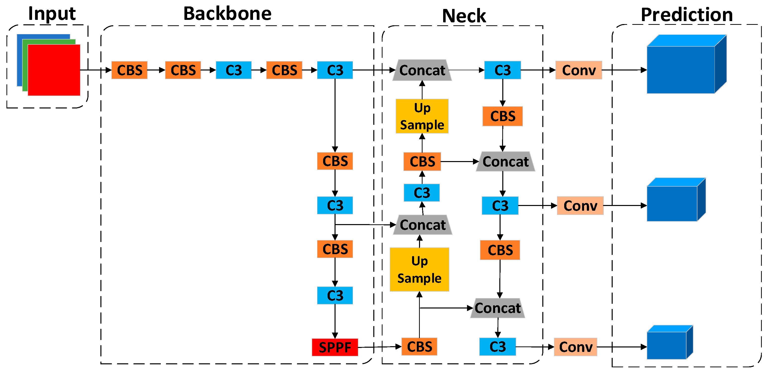
2.1. YOLOv5s Model
2.1.1. Input
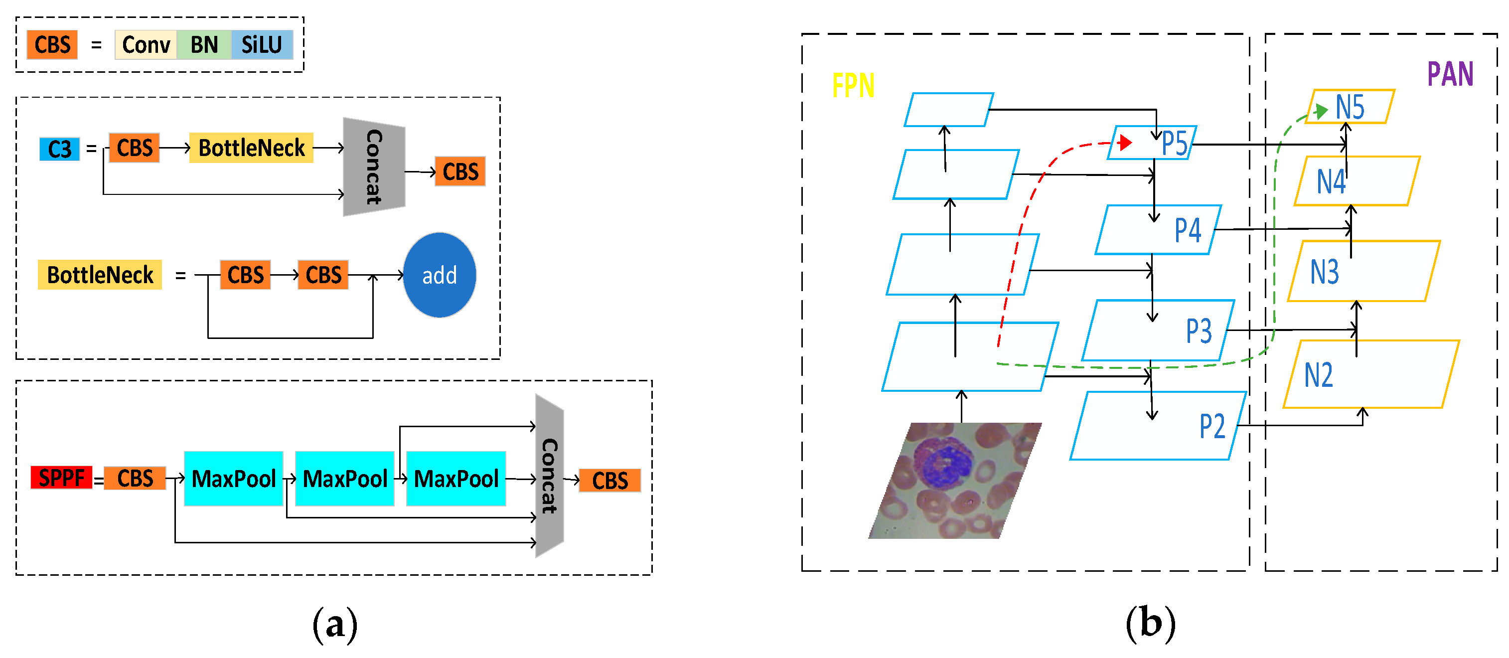
2.1.2. Backbone
2.1.3. Neck
2.1.4. Prediction
2.1.5. Loss
3. Proposed Method
3.1. Integration of the Swin Transformer Module
3.2. Improved the PANet Network Architecture
3.3. Improved Convolutional Structures in PAN
3.4. Improved IOU Loss Function
4. Experiments
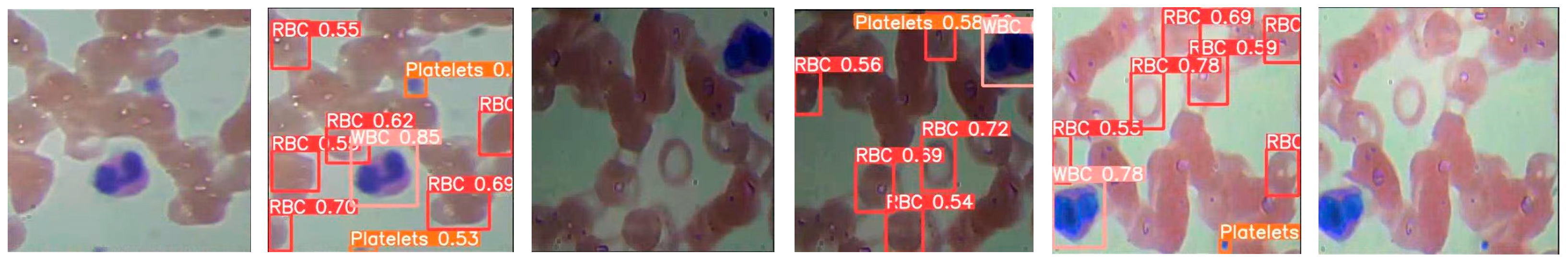
4.1. Dataset
4.2. Experimental Configuration
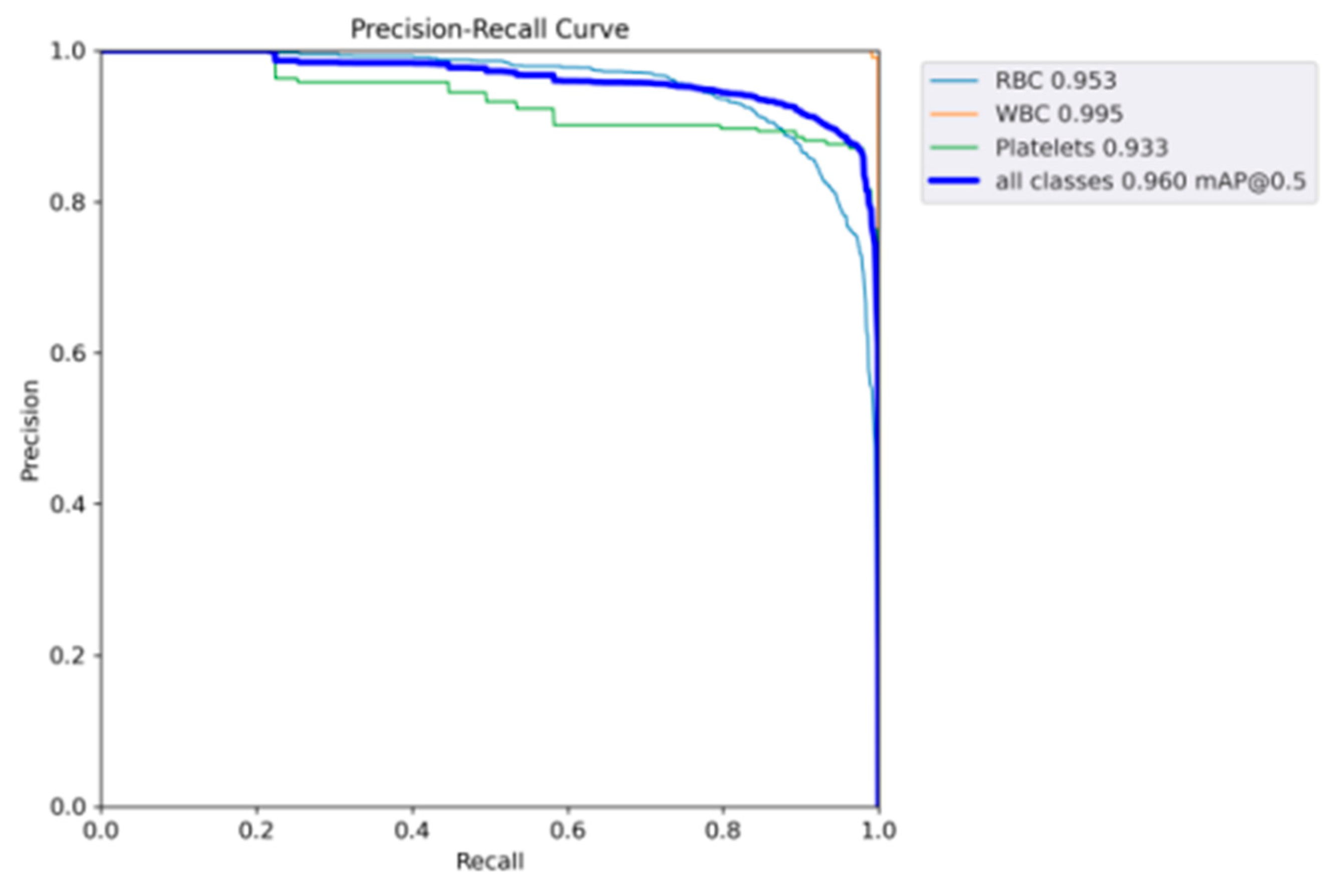
4.3. Evaluation Indicators
4.4. Results
5. Comparison with Other Datasets
6. Ablation Studies
7. Conclusions and Discussion
Author Contributions
Funding
Institutional Review Board Statement
Data Availability Statement
Conflicts of Interest
References
- Chen, Y. Study on the value of blood smear analysis in routine blood tests. China Pharm. Guide 2018, 16, 118–119. [Google Scholar]
- Chan, L.; Laverty, D. Accurate measurement of peripheral blood mononuclear cell concentration using image cytometry to eliminate RBC-induced counting error. J. Immunol. Methods 2013, 388, 25–32. [Google Scholar] [CrossRef] [PubMed]
- Lehmann, T.M.; Guld, M.O. Content-based image retrieval in medical applications. Methods Inf. Med. 2004, 43, 354–361. [Google Scholar] [PubMed]
- Patil, P.R.; Sable, G.S. Counting of WBCs and RBCs from blood images using gray thresholding. Int. J. Res. Eng. Technol. 2014, 3, 391–395. [Google Scholar]
- Reddy, V.H. Automatic red blood cell and white blood cell counting for telemedicine system. Int. J. Res. Advent Technol. 2014, 2, 294–299. [Google Scholar]
- Xiao, Q.; Huang, Y.B. Identification of diagnostic biomarkers for ulcerative colitis based on bioinformatics and machine learning. Chin. J. Immunol. 2023, 39, 1713–1718. [Google Scholar]
- Guo, J.B.; Zhang, T.H. A machine learning model based on gadoxetic acid disodium-enhanced MRI predicts microvascular invasion in hepatocellular carcinoma. J. Mol. Imaging 2023, 46, 736–740. [Google Scholar]
- Liu, Y.; Tian, J.; Hu, R. Improved feature point pair purification algorithm based on SIFT during endoscope image stitching. Front. Neurorobot. 2022, 16, 840594. [Google Scholar] [CrossRef]
- Guo, H.; Ding, J.Y. Research progress on the application of machine learning in the diagnosis and treatment of novel coronavirus infection. PLA Med. J. 2023, 48, 863–870. [Google Scholar]
- Zhuang, Y.; Jiang, N.; Xu, Y. Progressive distributed and parallel similarity retrieval of large CT image sequences in mobile telemedicine networks. Wirel. Commun. Mob. Comput. 2022, 2022, 1–13. [Google Scholar] [CrossRef]
- Wang, F.; Yan, J.H. Application of machine learning in leukaemia. Med. Rev. 2022, 28, 1928–1934. [Google Scholar]
- Guo, R.; Song, Z.J. Machine learning: The future of artificial intelligence. Electron. World 2018, 15, 33–35. [Google Scholar]
- Zhu, Y.; Huang, R.; Wu, Z. Deep learning-based predictive identification of neural stem cell differentiation. Nat. Commun. 2021, 12, 2614. [Google Scholar] [CrossRef] [PubMed]
- Yu, J.H.; Gao, H.W. Adaptive spatiotemporal representation learning for skeleton-based human action recognition. IEEE Trans. Cogn. Dev. Syst. 2021, 14, 1654–1665. [Google Scholar] [CrossRef]
- Ao, J.; Shao, X.; Liu, Z. Stimulated Raman scattering microscopy enables gleason scoring of prostate core needle biopsy by a convolutional neural network. Cancer Res. 2023, 83, 641–651. [Google Scholar] [CrossRef]
- Yu, J.H.; Gao, H.W. Deep temporal model-based identity-aware hand detection for space human–robot interaction. IEEE Trans. Cybern. 2021, 52, 13738–13751. [Google Scholar] [CrossRef]
- Li, M.; Mu, C.C. Application of deep learning in differential diagnosis of enamel cell tumour and odontogenic keratocyst based on surface lamellar slices. J. Chin. Acad. Med. Sci. 2023, 45, 273–279. [Google Scholar]
- Yu, J.H.; Gao, H.W.; Sun, J.; Zhou, D.L.; Ju, Z.J. Spatial cognition-driven deep learning for car detection in unmanned aerial vehicle imagery. IEEE Trans. Cogn. Dev. Syst. 2021, 14, 1574–1583. [Google Scholar] [CrossRef]
- Zhu, H.; Zhou, S.Y. A review of single-stage target detection algorithms based on deep learning. Ind. Control. Comput. 2023, 36, 101–103. [Google Scholar]
- Ye, J.X. A review of two-stage target detection algorithms based on deep learning. Internet Wkly. 2023, 18, 16–18. [Google Scholar]
- Wen, X.L.; Bai, T. Design of audio emotion recognition and classification model based on improved multimodal RCNN. Mod. Electron. Technol. 2023, 46, 114–118. [Google Scholar]
- Ren, S.Q.; He, K.; Girshick, R. Faster R-CNN: Towards Real-Time Object Detection with Region Proposal Networks. IEEE Trans. Pattern Anal. Mach. Intell. 2017, 39, 1137–1149. [Google Scholar] [CrossRef]
- Yang, H.Z.; Li, D. YOLOv4 target detection based on improved SPPnet. Electron. Prod. 2021, 12, 52–54. [Google Scholar]
- Qiao, Y.M.; Shi, J.K. Enhanced FPN underwater small target detection with improved loss function. J. Comput. Aided Des. Graph. 2023, 35, 525–537. [Google Scholar]
- Chen, D.H.; Sun, S.R.; Wang, Y.C. Research on improved SSD algorithm for small target detection. Sens. Microsyst. 2023, 42, 65–68. [Google Scholar]
- Yan, W.J.; Dai, J.H. Traffic sign recognition based on improved YOLOv3. J. Wuhan Eng. Vocat. Technol. Coll. 2023, 35, 31–35. [Google Scholar]
- Chen, Y.F.; Yan, C.C.; Zhou, C. Improved YOLOv4-based vehicle detection for autonomous driving scenarios. Autom. Instrum. 2023, 38, 59–63. [Google Scholar]
- Wang, Y.W.; Jiao, L.B. Remote Sensing target detection based on improved YOLOv5s. Comput. Meas. Control. 2023, 31, 70–76. [Google Scholar]
- Wang, F.X.; He, L.H. Research on weakly supervised melanoma image segmentation based on attention mechanism. Comput. Knowl. Technol. 2023, 19, 12–14. [Google Scholar]
- Ren, X.L. A study of attentional mechanisms and their role in medical visual tasks. Imaging Technol. 2023, 35, 76–80. [Google Scholar]
- Chen, C.Y.; Xu, B.W. A review of research on attention mechanisms in medical image processing. Comput. Eng. Appl. 2022, 58, 23–33. [Google Scholar]
- Yu, E.Z.; Zuo, X. Remote sensing ship image classification based on attention mechanism. Softw. Guide 2023, 22, 138–143. [Google Scholar]
- Fang, Z.C.; Wu, S.J. Application of image classification algorithm based on soft attention mechanism in defect detection. Mod. Inf. Technol. 2023, 7, 151–154. [Google Scholar]
- Fu, C.; Zhang, M. Anomalous brain MRI segmentation method incorporating texture features and attention mechanism. Print. Digit. Media Technol. Res. 2023, 12, 203–211. [Google Scholar]
- Fang, Y.; Jiang, Z. Insulator defect detection based on attention mechanism and feature fusion. Mod. Electron. Technol. 2023, 46, 49–54. [Google Scholar]
- Ren, H.S.; Zhou, Z.Y. Indoor scene depth map complementation based on channel attention mechanism. J. Zhejiang Univ. Technol. 2023, 49, 344–352. [Google Scholar]
- Wang, X.J.; Qian, R.R. A low-light image enhancement method combining spatial attention mechanism and multi-scale resolution fusion. Laser J. 2023, 44, 86–91. [Google Scholar]
- Wang, R.Q.; Wang, H.Q. Fusion of detail features and hybrid attention mechanism for fire smoke detection. Liq. Cryst. Disp. 2022, 37, 900–912. [Google Scholar] [CrossRef]
- Zheng, C.W.; Lin, H. A YOLOv5 helmet wearing detection method based on Swin Transformer. Comput. Meas. Control. 2023, 31, 15–21. [Google Scholar]
- Li, J.Q.; Zhang, L. An improved method for expression recognition based on depth-separable convolution. Intell. Comput. Appl. 2023, 13, 58–63. [Google Scholar]
- Zhang, Y.F.; Ren, W.; Zhang, Z. Focal and efficient IOU loss for accurate bounding box regression. Neurocomputing 2022, 506, 146–157. [Google Scholar] [CrossRef]
- Ouyang, D.; Huang, H.; Li, J. Improved yolov5s model for aerial image target detection algorithm. Fujian Comput. 2023, 39, 7–15. [Google Scholar]
- He, K.; Zhang, X.; Ren, S. Deep residual learning for image recognition. In Proceedings of the IEEE Conference on Computer Vision and Pattern Recognition, Las Vegas, NV, USA, 26 June–7 July 2016; pp. 770–778. [Google Scholar]
- Shah, S.A.R.; Wu, W.; Lu, Q. AmoebaNet: An SDN-enabled network service for big data science. J. Netw. Comput. Appl. 2018, 119, 70–82. [Google Scholar] [CrossRef]
- Chollet, F. Xception: Deep learning with depth wise separable convolutions. In Proceedings of the IEEE Conference on Computer Vision and Pattern Recognition, Honolulu, HI, USA, 21–26 July 2017; pp. 1251–1258. [Google Scholar]
- Lin, T.Y.; Dollar, P.; Girshick, R. Feature pyramid networks for object detection. In Proceedings of the IEEE Conference on Computer Vision and Pattern Recognition, Honolulu, HI, USA, 21–26 July 2017; pp. 2117–2125. [Google Scholar]
- Liu, S.; Qi, L.; Qin, H. Path aggregation network for instance segmentation. In Proceedings of the IEEE Conference on Computer Vision and Pattern Recognition, Salt Lake City, UT, USA, 18–22 June 2018; pp. 8759–8768. [Google Scholar]
- Available online: https://github.com/Shenggan/BCCD_Dataset (accessed on 24 February 2018).
- Wang, Y.F.; Li, D.H. Improved blood cell detection algorithm for YOLO framework. Comput. Eng. Appl. 2022, 58, 191–198. [Google Scholar]
- Ahmad, M.; Qadri, S.F.; Ashraf, M.U. Efficient liver segmentation from computed tomography images using deep learning. Comput. Intell. Neurosci. 2022, 2022, 2665283. [Google Scholar] [CrossRef] [PubMed]
- Qadri, S.F.; Lin, H.; Shen, L. CT-Based Automatic Spine Segmentation Using Patch-Based Deep Learning. Int. J. Intell. Syst. 2023, 2023, 2345835. [Google Scholar] [CrossRef]
- Xu, F.; Li, X.; Yang, H. TE-YOLOF: Tiny and efficient YOLOF for blood cell detection. Biomed. Signal Process. Control. 2022, 73, 103416. [Google Scholar] [CrossRef]
- Liu, C.; Li, D.; Huang, P. ISE-YOLO: Improved Squeeze-and-Excitation Attention Module based YOLO for Blood Cells Detection. In Proceedings of the 2021 IEEE International Conference on Big Data, Orlando, FL, USA, 15–18 December 2021; pp. 3911–3916. [Google Scholar]
- Available online: https://luna16.grand-challenge.org (accessed on 20 October 2020).
- Huang, S.A. Traffic sign detection based on improved YOLO model. Sci. Technol. Innov. 2021, 18, 194–196. [Google Scholar]


| Parameter Name | Parameter Values | Parameter Name | Parameter Values |
|---|---|---|---|
| Batch size | 16 | Epoch | 133 |
| Learning rate | 0.01 | Momentum | 0.937 |
| Box loss | 0.05 | Cls loss | 0.5 |
| Anchors | (10, 13), (16, 30), 33, 23), (30, 61), (62, 45), (59,119) | Obj loss | 1.0 |
| Method | Input Size | WBCs | RBCs | Platelets | mAP | FPS |
|---|---|---|---|---|---|---|
| Fast-RCNN [22] | 1000 600 | 0.803 | 0.722 | 0.770 | 0.765 | 9.2 |
| YOLOv3 [26] | 608 608 | 0.914 | 0.829 | 0.774 | 0.839 | 34.5 |
| YOLOv4 [27] | 640 640 | 0.930 | 0.798 | 0.813 | 0.847 | 36.1 |
| TE-YOLOF-B3 [52] | 416 416 | 0.987 | 0.873 | 0.898 | 0.919 | 43 |
| ISE-YOLO [53] | 416 416 | 0.965 | 0.927 | 0.896 | 0.857 | 34.5 |
| YOLOv5s [42] | 640 640 | 0.977 | 0.838 | 0.873 | 0.896 | 56.7 |
| SDE-YOLO | 640 640 | 0.995 | 0.953 | 0.933 | 0.960 | 43.4 |
| Method | Input Size | WBCs | RBCs | Platelets | mAP | FPS | F1_curve | Precision |
|---|---|---|---|---|---|---|---|---|
| YOLOv7 | 640 × 640 | 0.995 | 0.954 | 0.928 | 0.959 | 9.1 | 0.92 | 0.864 |
| YOLOv8 | 640 × 640 | 0.995 | 0.960 | 0.945 | 0.967 | 54.8 | 0.93 | 0.807 |
| SDE-YOLO | 640 × 640 | 0.995 | 0.953 | 0.933 | 0.960 | 43.4 | 0.92 | 0.851 |
| Method | Input Size | WBCs | RBCs | Platelets | mAP | F1_curve | Precision |
|---|---|---|---|---|---|---|---|
| YOLOv5s [42] | 640 × 640 | 0.977 | 0.838 | 0.873 | 0.896 | 0.90 | 0.858 |
| YOLOv5s + A | 640 × 640 | 0.995 | 0.949 | 0.959 | 0.968 | 0.93 | 0.922 |
| YOLOv5s + B | 640 × 640 | 0.991 | 0.938 | 0.953 | 0.961 | 0.92 | 0.892 |
| YOLOv5s + C | 640 × 640 | 0.995 | 0.959 | 0.945 | 0.966 | 0.92 | 0.865 |
| YOLOv5s + D | 640 × 640 | 0.995 | 0.950 | 0.967 | 0.971 | 0.93 | 0.888 |
| YOLOv5s + A + B | 640 × 640 | 0.957 | 0.899 | 0.955 | 0.937 | 0.91 | 0.889 |
| YOLOv5s + A + C | 640 × 640 | 0.995 | 0.957 | 0.958 | 0.970 | 0.93 | 0.898 |
| YOLOv5s + A + D | 640 × 640 | 0.995 | 0.950 | 0.953 | 0.966 | 0.93 | 0.920 |
| YOLOv5s + B + C | 640 × 640 | 0.995 | 0.953 | 0.954 | 0.967 | 0.92 | 0.970 |
| YOLOv5s + B + D | 640 × 640 | 0.995 | 0.945 | 0.954 | 0.965 | 0.92 | 0.861 |
| YOLOv5s + C + D | 640 × 640 | 0.995 | 0.937 | 0.945 | 0.959 | 0.91 | 0.888 |
| YOLOv5s + A + B + C | 640 × 640 | 0.995 | 0.948 | 0.953 | 0.965 | 0.92 | 0.862 |
| YOLOv5s + A + C + D | 640 × 640 | 0.995 | 0.948 | 0.955 | 0.966 | 0.93 | 0.909 |
| YOLOv5s + B + C + D | 640 × 640 | 0.995 | 0.939 | 0.958 | 0.964 | 0.92 | 0.904 |
| SDE-YOLO | 640 × 640 | 0.995 | 0.953 | 0.933 | 0.960 | 0.92 | 0.902 |
Disclaimer/Publisher’s Note: The statements, opinions and data contained in all publications are solely those of the individual author(s) and contributor(s) and not of MDPI and/or the editor(s). MDPI and/or the editor(s) disclaim responsibility for any injury to people or property resulting from any ideas, methods, instructions or products referred to in the content. |
© 2023 by the authors. Licensee MDPI, Basel, Switzerland. This article is an open access article distributed under the terms and conditions of the Creative Commons Attribution (CC BY) license (https://creativecommons.org/licenses/by/4.0/).
Share and Cite
Wu, Y.; Gao, D.; Fang, Y.; Xu, X.; Gao, H.; Ju, Z. SDE-YOLO: A Novel Method for Blood Cell Detection. Biomimetics 2023, 8, 404. https://doi.org/10.3390/biomimetics8050404
Wu Y, Gao D, Fang Y, Xu X, Gao H, Ju Z. SDE-YOLO: A Novel Method for Blood Cell Detection. Biomimetics. 2023; 8(5):404. https://doi.org/10.3390/biomimetics8050404
Chicago/Turabian StyleWu, Yonglin, Dongxu Gao, Yinfeng Fang, Xue Xu, Hongwei Gao, and Zhaojie Ju. 2023. "SDE-YOLO: A Novel Method for Blood Cell Detection" Biomimetics 8, no. 5: 404. https://doi.org/10.3390/biomimetics8050404
APA StyleWu, Y., Gao, D., Fang, Y., Xu, X., Gao, H., & Ju, Z. (2023). SDE-YOLO: A Novel Method for Blood Cell Detection. Biomimetics, 8(5), 404. https://doi.org/10.3390/biomimetics8050404