Abstract
The slime mold algorithm (SMA) and the arithmetic optimization algorithm (AOA) are two novel meta-heuristic optimization algorithms. Among them, the slime mold algorithm has a strong global search ability. Still, the oscillation effect in the later iteration stage is weak, making it difficult to find the optimal position in complex functions. The arithmetic optimization algorithm utilizes multiplication and division operators for position updates, which have strong randomness and good convergence ability. For the above, this paper integrates the two algorithms and adds a random central solution strategy, a mutation strategy, and a restart strategy. A hybrid slime mold and arithmetic optimization algorithm with random center learning and restart mutation (RCLSMAOA) is proposed. The improved algorithm retains the position update formula of the slime mold algorithm in the global exploration section. It replaces the convergence stage of the slime mold algorithm with the multiplication and division algorithm in the local exploitation stage. At the same time, the stochastic center learning strategy is adopted to improve the global search efficiency and the diversity of the algorithm population. In addition, the restart strategy and mutation strategy are also used to improve the convergence accuracy of the algorithm and enhance the later optimization ability. In comparison experiments, different kinds of test functions are used to test the specific performance of the improvement algorithm. We determine the final performance of the algorithm by analyzing experimental data and convergence images, using the Wilcoxon rank sum test and Friedman test. The experimental results show that the improvement algorithm, which combines the slime mold algorithm and arithmetic optimization algorithm, is effective. Finally, the specific performance of the improvement algorithm on practical engineering problems was evaluated.
1. Introduction
In the past decade, the exploitation and application of optimization models have begun to receive attention from mathematicians and engineers. In recent years, with the continuous exploitation of computer technology, more and more optimization problems have attracted people’s attention. The unconstrained optimization problem is currently a research hotspot. The complexity of these problems is gradually increasing, and they have characteristics such as being large-scale, multimodal, and nonlinear [1]. The meta-heuristic algorithm has become an excellent tool and has been recognized by people because it is simple, easy to implement, does not require gradient information, and can avoid local optimization [2]. This is because the meta-heuristic algorithm treats the problem as a black box model and only needs to input the problem to obtain the output of the problem. Researchers develop meta-heuristic algorithms by simulating various natural phenomena and biological habits. Meta-heuristic algorithms can effectively handle real-life optimization problems because they possess valuable randomness that allows them to bypass local optima and have stronger search capabilities than traditional optimization algorithms. These valuable characteristics of the meta-heuristic algorithm make it very smooth when dealing with application problems. Examples include neural networks [3], clustering [4], engineering [5], and scheduling problems [6].
The main problem is whether a meta-heuristic algorithm can be used to solve most of the problems. No Free Lunch (NFL) [7] explains that when an algorithm can provide a good solution to a particular problem, it is not guaranteed a good result on other problems. NFL’s law motivates researchers to enhance their ability to solve new problems by improving currently known algorithms. For example, Chen et al. were inspired by the lifestyle of beluga whales and developed an IBWO [8] that improved the algorithm’s global optimization ability; Wen et al. enhanced the global optimization capability of the algorithm by using a new host-switching mechanism [9]; Wu et al. improved the sand cat’s wandering strategy and applied it to engineering problems [10].
AOA [11] is a meta-heuristic optimization algorithm designed based on the four mixed operations proposed by Abualigah et al. in 2021. The algorithm uses multiplication and division operations in mathematics to improve the global dispersion of position updates and addition and subtraction operations to improve the accuracy of position updates in local areas. However, AOA still faces problems such as slow convergence in complex environments. It needs further improvement and perfecting to adapt to more complex optimization problems. Recently, many researchers have made improvements to the AOA, including adaptive parallel arithmetic optimization algorithm (AAOA) [12], dynamic arithmetic optimization algorithm (DAOA) [13], and chaotic arithmetic optimization algorithm (CAOA) [14].
SMA [15] is a new swarm intelligence optimization algorithm proposed by Li et al. in 2020 to simulate slime mold’s behavior and morphological changes in the foraging process. Its inspiration comes from simulating the foraging behavior and morphological changes of physarum polycephalum and using the weight change to simulate the positive feedback and negative feedback processes generated by slime molds in the foraging process, thus generating three stages of foraging patterns. The SMA has strong global exploration ability, certain convergence accuracy, and good stability, but in the later iteration stage, the oscillation effect is weak, and it is easy to fall into local optima. The contraction mechanism is not strong, resulting in a slower convergence speed. At present, researchers have improved and widely used this algorithm. Kouadri et al. [16] applied the algorithm to solve the problem of minimizing fuel costs and losses in exploration generators. Zhao et al. [17] proposed mixing SMA and HHO algorithms, utilizing multiple composite selection mechanisms to improve the algorithm’s selectivity and randomness, the randomness of individual position updates, and the efficiency of algorithm solving.
Based on the advantages and disadvantages of SMA and AOA, this article aims to create a more effective optimization algorithm by combining the two algorithms. To further enhance its performance, a random center solution strategy is introduced. This strategy uses random center learning to expand the exploration range of individual populations, enrich population diversity, and can effectively control the balance between exploration and exploitation. Both mutation strategy and restart strategy were used. The mutation strategy is a local adaptive mutation method that improves the algorithm’s global search ability and performs well in high-dimensional spaces. The restart strategy can help poorer individuals jump to other positions and is usually used to jump out of local optima. The proposed mixed optimization algorithm, hybrid slime mold and arithmetic optimization algorithm with random center learning and restart mutation (RCLSMAOA), incorporates the best features of both SMA and AOA, making it more effective in exploring the search space and enabling it to effectively solve corresponding engineering problems. The algorithm focuses on improving four key aspects:
- (1)
- In the exploration and exploitation stage, SMA and AOA should be organically combined to improve the exploration and exploitation capabilities comprehensively;
- (2)
- Innovatively propose a random center strategy, which improves the early convergence speed of the algorithm and effectively maintains a balance between exploration and development while enhancing the diversity of the population;
- (3)
- The introduction of the mutation strategy and restart strategy enhances the ability to solve complex problems while also enhancing the algorithm’s ability to jump out of local optima. By comparing 23 benchmark test functions with different dimensions with the CEC2020 test function, it is proven that the algorithm has significant effectiveness;
- (4)
- Five engineering problems were used simultaneously to verify the feasibility of RCSMAOA on practical engineering problems.
The second part of this article introduces the relevant work. SMA and AOA were introduced in the third and fourth parts, respectively. In the fifth part, we described the added strategies; SCLS, MS, and RS explained the implementation process of the algorithm and provided pseudocode and flowchart. The sixth part is the analysis of time complexity. The seventh part is the experimental analysis of the specific performance of RCLSMAOA. The eighth part is the application of RCLSMAOA in specific engineering problems. The ninth part summarizes the contributions of this article and introduces the next research directions. If you need the code in our article, you can find it through the following link: https://github.com/Mars02w/RCLSMAOA, accessed on 20 August 2023.
2. Related Works
In recent years, meta-heuristic algorithms can be divided into the following four categories based on their inspiration sources: (1) physics-based methods, whose inspiration comes from physical rules in the universe. Specific algorithms include the black hole algorithm (BH) [18], the gravity search algorithm (GSA) [19], and the most famous simulated annealing algorithm (SA) [20]. (2) Evolution-based algorithms inspired by the laws of biological evolution. Researchers have linked natural and artificial evolution to create many excellent algorithms. Examples include genetic algorithm (GA) [21], genetic programming (GP) [22], and differential evolution (DE) [23]. (3) Group-based algorithms focus on modeling observations of animals and other living organisms. The most famous is particle swarm optimization (PSO) [24], which simulates the behavior of birds and fish. Ant Colony Algorithm (ACO) [25] simulates the behavior of ants searching for food sources. The foraging behavior of slime molds inspires the slime mold optimization algorithm (SMA) [15]. (4) Human behavior habits and ideas inspire human-based algorithms in social life. A well-known one is the teaching–learning-based optimizer (TLBO) [26], inspired by the interaction between teachers and students. There are also training-based optimizers (DTBO) [27] and internal search algorithms (ISA) [28]. In recent years, many excellent algorithms have still been proposed by researchers, such as the monarch Butterfly optimization (MBO) [29], more search algorithm (MSA) [30], hunger games search (HGS) [31], Runge Kutta method (RUN) [32], colony prediction algorithm (CPA) [33], weighted mean of vectors (INFO) [34], Harris hawks optimization (HHO) [35], and prime optimization algorithm (RIME) [36].
In addition, studying hybrid optimization algorithms is also a new trend at present. In recent years, researchers have increasingly conducted mixed research on algorithms. For example, Alam Zeb et al. [37] mixed a genetic algorithm with a simulated annealing algorithm, and the powerful exploration ability of the genetic algorithm compensated for the lack of exploration in the simulated annealing algorithm, enhancing the actual optimization performance of the algorithm. Chen et al. [38] fused a particle swarm optimization algorithm with a simulated annealing algorithm and applied it to magnetic anomaly detection, achieving success. Hybrid optimization algorithms also have the ability to solve optimal power flow problems [39]. Tumari et al. studied a variant of the ocean predator algorithm for adjusting the fractional order proportional integral derivative controller of the automatic voltage regulator system [40]. Wang et al. [41] added an angle modulation mechanism to a dragonfly algorithm to enable it to work in two-dimensional space and have good performance. Devaraj A et al. [42] used a combination of fireflies and improved multi-objective particle swarm optimization (IMPSO) technology to improve load balancing capabilities in cloud computing environments and the results showed success. Jui et al. [43] hybridized the average multi-verse optimizer and sine cosine algorithm, demonstrating good potential in solving continuous-time Hammerstein system problems.
3. Slime Mold Algorithm
The SMA is a meta-heuristic optimization algorithm that simulates the foraging behavior of slime molds. This algorithm reflects slime molds’ oscillation and contraction characteristics during the foraging process. The organic matter in slime molds first secretes enzymes when searching for food, and then during migration, the front end extends into a fan shape and uses a venous network for foraging. Due to their unique morphology and characteristics, they can simultaneously utilize multiple pathways to form a connected venous network to obtain food. In addition, slime molds will also search for food in other unknown areas.
When the slime mold vein is close to food according to the smell in the air, the higher the food concentration, the stronger the propagation wave generated by the biological oscillator in its body, which increases the flow of cytoplasm in the vein. The faster the flow of cytoplasm, the thicker the slime mold vein tube, which causes the position update of the slime mold. The position update formula is:
where Xb(t) represents the current position of the individual with the optimal fitness, vb is a parameter between [-a,a], W represents the weight coefficients of the slime mold, Xrand1(t) and Xrand2(t) represent the positions of two randomly selected individuals, r1 represents the random number in the interval [0, 1], vc is the parameter that linearly decreases from 1 to 0, and t is the current number of iterations.
The updating formula of control parameters a, p, and weight coefficient W is as follows:
The parameters are calculated based on the current individual’s fitness and optimal values, where i = 1,2,…, N. N represents the number of populations, S(i) represents the fitness value of the ith slime mold individual, and DF represents the optimal fitness obtained in the current iteration process. T represents the maximum number of iterations, and r2 is a random number within the [0, 1] interval. condition are the individuals whose fitness is in the top half of the population, and others are the remaining individuals. bF represents the best fitness value obtained during the current iteration, and wF represents the worst fitness value obtained during the current iteration. SIndex(i) indicates the fitness value sequence.
Even if slime molds find a food source, they will separate some individuals to explore other unknown areas to find a higher-quality food source. At this point, the formula for the slime mold update position is as follows:
Among them, rand is a random number within the [0, 1] interval, UB and LB represent upper and lower bounds, and z represents a custom parameter (with a value of 0.03).
4. Arithmetic Optimization Algorithm
AOA is a meta-heuristic optimization algorithm exploring and exploiting mechanisms through arithmetic operators in mathematics. The exploration stage refers to using multiplication (M) and division (D) strategies for extensive coverage and search space, improving the dispersion of solutions to avoid local optima. The exploitation stage is to improve the accuracy of the solutions obtained in the exploration stage through the addition (A) strategy and the subtraction (S) strategy, that is, to enhance the local optimization ability.
4.1. Mathematical Optimization Acceleration Function
Before exploration and exploitation, AOA generates a math optimizer accelerated (MOA) to select the search phase. When r1 > MOA (t), the exploration phase is carried out by executing (D) or (M); when r1 ≤ MOA (t), the exploitation phase is carried out by executing (A) or (S); r1 is a random number from 0 to 1.
where Min and Max represent the minimum and maximum values of the optimization acceleration function (MOA).
4.2. Exploration Phase
AOA looks at different parts of the search space (global optimization) using two main search methods (multiplication (M) search strategy and division (D) search strategy). It updates its position using this formula:
where r2 ∈ [0, 1], Xi,j(t + 1) is the position of the ith individual on the jth dimension during the next iteration. Xb,j(t) is the location of the best solution for the current fitness. ɛ is a very small number, where UBj and LBj represent the upper and lower limits of the jth position, respectively. µ is the control parameter for adjusting the search process, which is 0.499.
The Mathematical Optimizer Probability (MOP) is a coefficient, α is a sensitive parameter that defines the exploitation accuracy during the iteration process, which is fixed at 5.
4.3. Exploitation Phase
AOA utilizes operators (subtraction (S) and addition (A)) to deeply explore search areas in several dense areas and conducts local optimization based on two main exploitation strategies. The location update formula is as follows:
Among them, r3 is a random number between 0 and 1.
5. Hybrid Improvement Strategy
5.1. Stochastic Center Learning Strategy (SCLS)
The random center learning strategy is a newly proposed optimization mechanism in this paper. In nature, group animals such as wolf packs and whale packs often surround their food in the middle through group cooperation and then engage in predation. In this regard, this article proposes a central learning strategy whose core idea is to generate a central solution based on upper and lower bounds during the process of searching for the optimal value of the population, comparing it with the target fitness value of the existing optimal solution, and selecting the optimal one for the next iteration. Definition of the central solution: if there is a point X in the n-dimensional coordinate system, then the central solution is calculated as follows:
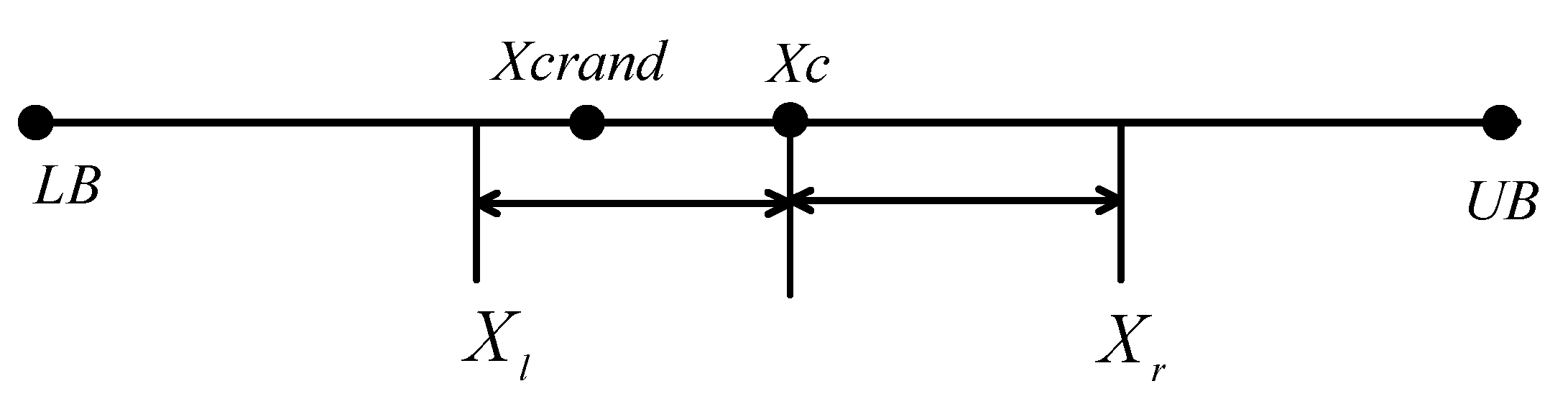
Among them, Xc is the central solution. Due to the lack of randomness in the central solution. In order to further improve the ability of the population to find the globally optimal solution (as shown in Figure 1), this paper proposes an improved random center learning strategy, which is calculated as follows:
where Xcrand represents the random central solution, Xr and Xl represent the object to be learned, and r1, r2, and rand are random numbers between 0 and 1. In order to reflect the randomness and symmetry of the value of random center learning, the threshold value of rand () is 0.5. The schematic diagram of the central solution and random central learning is shown in Figure 1.

Figure 1.
Central solution and random central learning solution.
Figure 1 shows that any position in the interval [Xl, Xr] may have a random central solution Xcrand, with Xc being the central solution.
5.2. Mutation Strategy (MS)
Mutation strategy refers to a composite mutation strategy based on multiple mutation operators in the mutation strategy [44]. It generates three candidate positions Vi1, Vi2, and Vi3, for the ith position by executing Equations (13)–(15) in parallel. The formula is as follows:
Among them, Xrk, j represents the jth dimension of the rk solution (the same below), r1, r2, and r3 are different integers in the range [1, N], jrand represents integers in the interval [1, D], F1 represents a proportional coefficient equal to 1.0, and Cr1 represents a crossover rate set to 0.1.
r4, r5, r6, r7, and r8 are distinct integers in the range [1, N]. F2 represents a proportional coefficient equal to 0.8, and Cr2 represents a crossover rate equal to 0.2.
r9, r10, and r11 are distinct integers in the range [1, N]. F3 represents a proportional coefficient equal to 1.0, and Cr3 represents a crossover rate of 0.9.
After generating three candidate positions Vi1, Vi2, and Vi3, first correct them based on the upper and lower boundaries. Then, select the candidate solution Vi with the best fitness from Vi1, Vi2, and Vi3 to update the position of the ith solution using Formula (16), which is called a greedy selection strategy, as shown below.
Vi represents the modified best candidate solution, and Xi represents the ith position.
5.3. Restart Strategy (RS)
When the mucus cannot find food at this location for a long time, it means that the nutrients in the area are no longer sufficient to support the continued survival of the slime molds, so the slime molds in the area need to be relocated. The restart scheme [9] can help poorer individuals transition from a local optimal state to other positions, so we use a restart strategy here to change the position of poorer individuals. In this strategy, we use the trial vector trial(i) to record the number of times the position has not improved. If the fitness value corresponding to the position in the search does not improve, the test vector trial(i) increases by 1. Otherwise, trial(i) is reset to 0. If the test vector is not less than the predetermined limit, a better vector will be selected from the test vectors T1 and T2 to replace the position of the ith.
where T1,j represents the jth dimension position in position T1, T2,j represents the jth position in position T2, UBj and LBj are the upper and lower boundaries of the jth dimension, respectively, and rand() represents the random floating-point arithmetic in the region [0, 1]. If T2,j exceeds the upper boundary UBj or lower boundary LBj in the jth dimension of the position, it will be replaced by Equations (18) and (19), and the test vector test trial (i) will be reset to zero. This article sets this limit to log t. If the restrictions are smaller in the early stages, they will help enhance the global performance of the algorithm. If the limit is larger in the later stage, it can prevent the algorithm from moving away from the optimal solution.
5.4. A Hybrid Optimization Algorithm of Slime Mold and Arithmetic Based on Random Center Learning and Restart Mutation
As mentioned above, when exploring unknown food sources, slime molds in SMA update their positions based on the synergistic effect of VB and Vc. The oscillation effect of VB increases the possibility of global exploration. When the random number z is less than, slime molds are initialized. At the end of the iteration, the VB oscillation effect is weakened, which makes the algorithm easily fall into the local optimum. Vc is a linearly decreasing parameter from 1 to 0, and the search mechanism is single and weak, making it difficult for the algorithm to jump out of local optima. In AOA, position updating is carried out according to the higher distribution of the division operator, and contraction is realized according to the addition and subtraction operators. The probability MOP of the mathematical optimizer changes according to the optimal position to improve the search breadth of exploration and increase the ability of the algorithm to jump out of the local optimum, but it will inevitably fall into the local optimum in the later iteration. The random center learning updates the random position according to the general characteristics of the optimal solution, which will improve the algorithm’s convergence rate in the early exploration stage. CMS introduces multiple candidate solutions and compares them with existing solutions. In RS, the number of times the position has not been improved is recorded using the experimental vector trial (i). When the given threshold is exceeded, it is preliminarily determined that the algorithm is trapped in a local optimum, and a new position update formula is given to prevent the algorithm from jumping out of the local optimum.
Therefore, in this paper, we abandon the weak mechanism in the exploration stage of SMA and add the multiplication and division operator in AOA to expand the scope of exploration. The mutation and restart strategies are introduced to improve the ability to jump out of the local optimal in the late iteration. Given the relatively slow convergence rate of the algorithm in the exploration stage, a random center learning strategy with characteristic solutions is added.
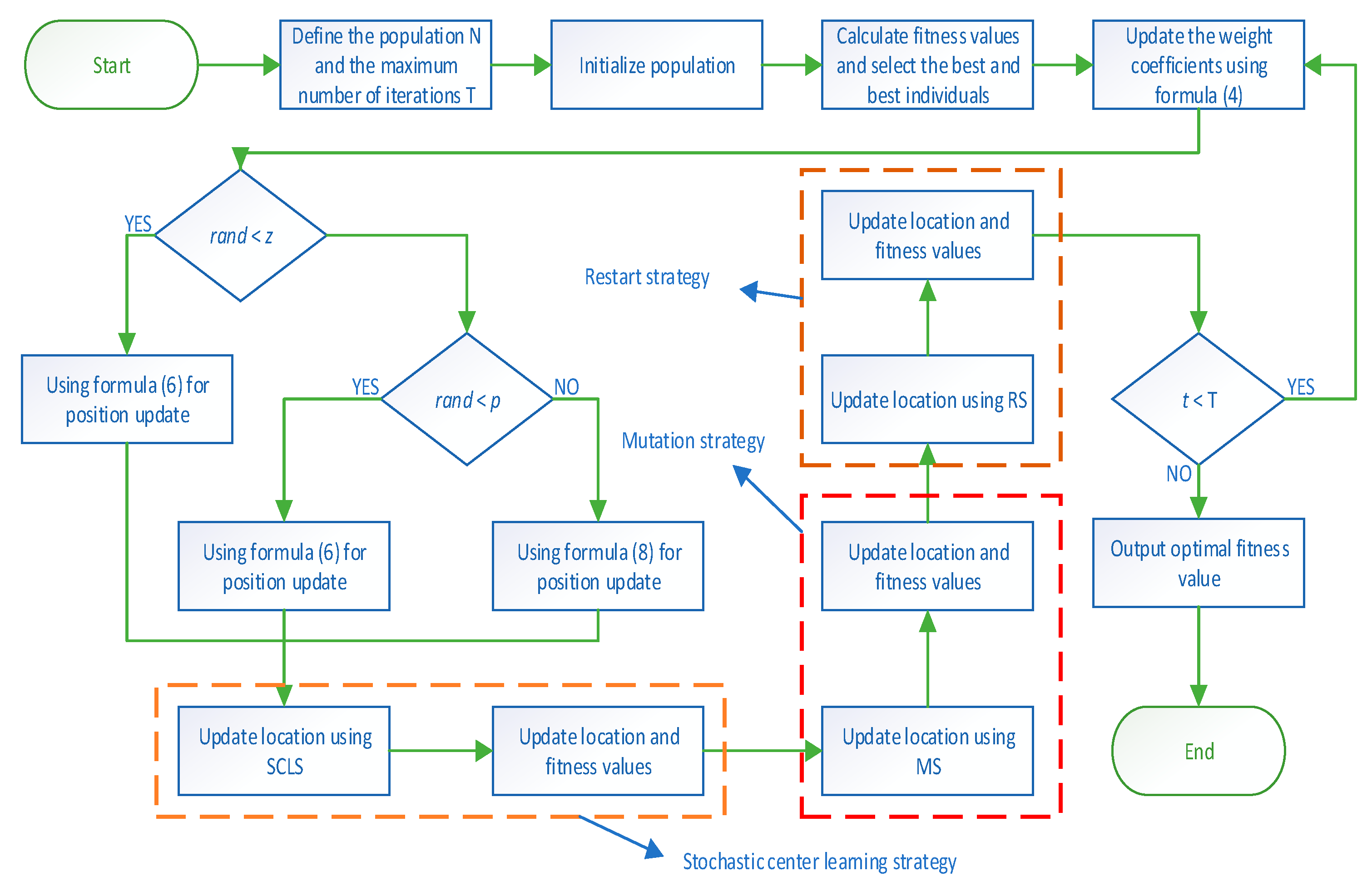
To sum up, the hybrid slime mold and arithmetic optimization algorithm with random center learning and restart mutation (RCLSMAOA) proposed in this paper, which integrates stochastic center learning, has advantages and balance in the exploration and exploitation stage, local optimization, and global optimization. Pseudocode as shown in Algorithm 1. The flowchart is shown in Figure 2.
| Algorithm 1 The pseudocode of the RCLSMAOA |
| Initialization parameters T, Tmax, ub, lb, N, dim, w. |
| Initialize population X according to Equation (1). |
| While T ≤ Tmax |
| Calculate fitness values and select the best individual and optimal location. |
| Update w using Formula (4) |
| For i = 1:N |
| Update the value of parameter a W S using Formulas (2), (4), and (5) |
| If rand < z |
| Update the population position using Formula (6) |
| Else |
| Update vb, vc, and p. |
| If r1 < p |
| Update the population position using Formula (6) |
| Else |
| Update the value of parameter mop using Formula (9) |
| If r2 < 0.5 |
| Update the population position using Formula (8) |
| Else |
| Update the population position using Formula (8) |
| End If |
| End If |
| End If |
| For i = 1:N |
| Update population position using SCLS |
| End For |
| For i = 1:N |
| Update population position using MS |
| End For |
| Update population position using RS |
| Find the current best solution |
| t = t + 1 |
| End While |
| Output the best solution. |
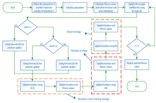
Figure 2.
Flow chart.
6. Time Complexity Analysis
In the RCLSMAOA, if the number of populations is N, the dimension is dim, and the maximum number of iterations is T. The time complexity of the population initialization phase is O(N × Dim). During iteration, the location of vb mechanism and AOA multiplication and division operator in SMA is updated, and the time complexity of the random central solution strategy and mutation strategy is O(3 × N × Dim × T). The time complexity of updating the convergence curve is O(1). It is worth mentioning that RS is rarely used from a general perspective, so it can be ignored and not remembered. In conclusion, the time complexity of the RCLSMAOA is O(N × Dim × (3T + 1)).
7. Experimental Part
All the experiments in this paper are completed on the computer with the 11th Gen Intel(R) Core(TM) i7-11700 processor with a primary frequency of 2.50 GHz, 16 GB memory, and an operating system of 64-bit Windows 11 using matlab2021a. In order to check the performance of the RCLSMAOA, 23 standard reference functions and CEC2020 reference functions are used to check the algorithm’s performance. In order to have a more comprehensive understanding of the actual performance of the RCLSMAOA, we choose different algorithms to compare. These include AOA and SMA, as well as the famous remora optimization algorithm (ROA) [37], sine cosine algorithm (SCA) [38], and whale optimization algorithm (WOA) [39]. In addition, we have added two improved algorithms: the whale and moth flame optimization algorithms and the average multi-verse optimizer and sine cosine algorithm. The parameter settings for these algorithms are shown in Table 1.

Table 1.
Parameter settings for the comparative algorithms.
7.1. Experiments on the 23 Standard Benchmark Functions
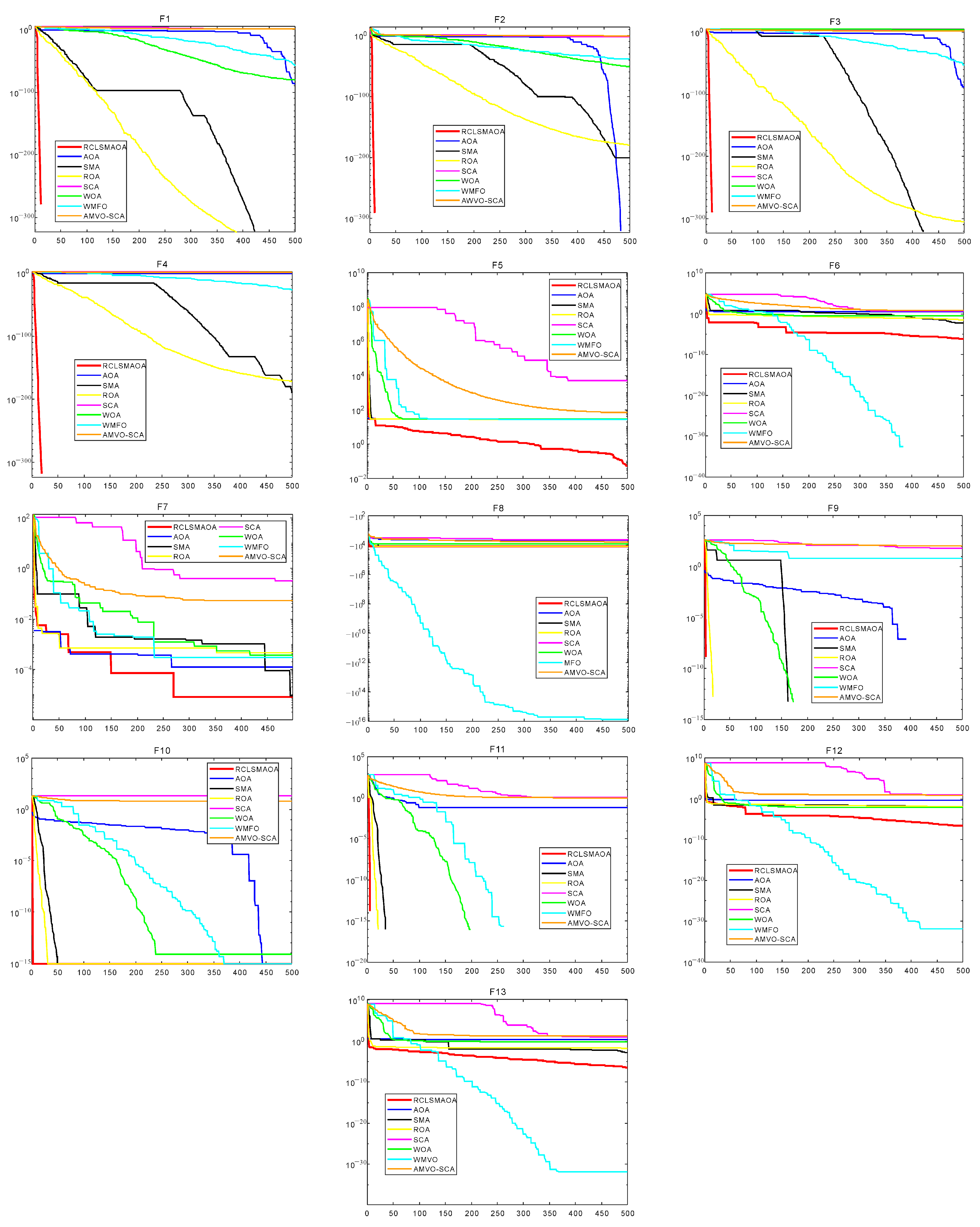
In this section, we selected 23 benchmark functions to test RCLSMAOA’s performance [10]. The 23 functions consist of 7 single-mode functions, six multimodal functions, and ten fixed multimodal functions. Fn(x) represents the specific mathematical expression of the reference function, dim is the experimental dimension of the reference function, the range is the search space of the reference function, and Fmin is the theoretical optimal value of the corresponding reference function. See Figure 3 for the image of the specific function. In this experiment, we set the population size N = 30, spatial dimension = 30/500, and the maximum number of iterations T = 500. RCLSMAOA and other comparison algorithms were run 30 times to obtain each algorithm’s best fitness, average fitness, and standard deviation after 30 times of independent running.
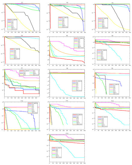
Figure 3.
F23 function images with dim = 30 (F1–F13).
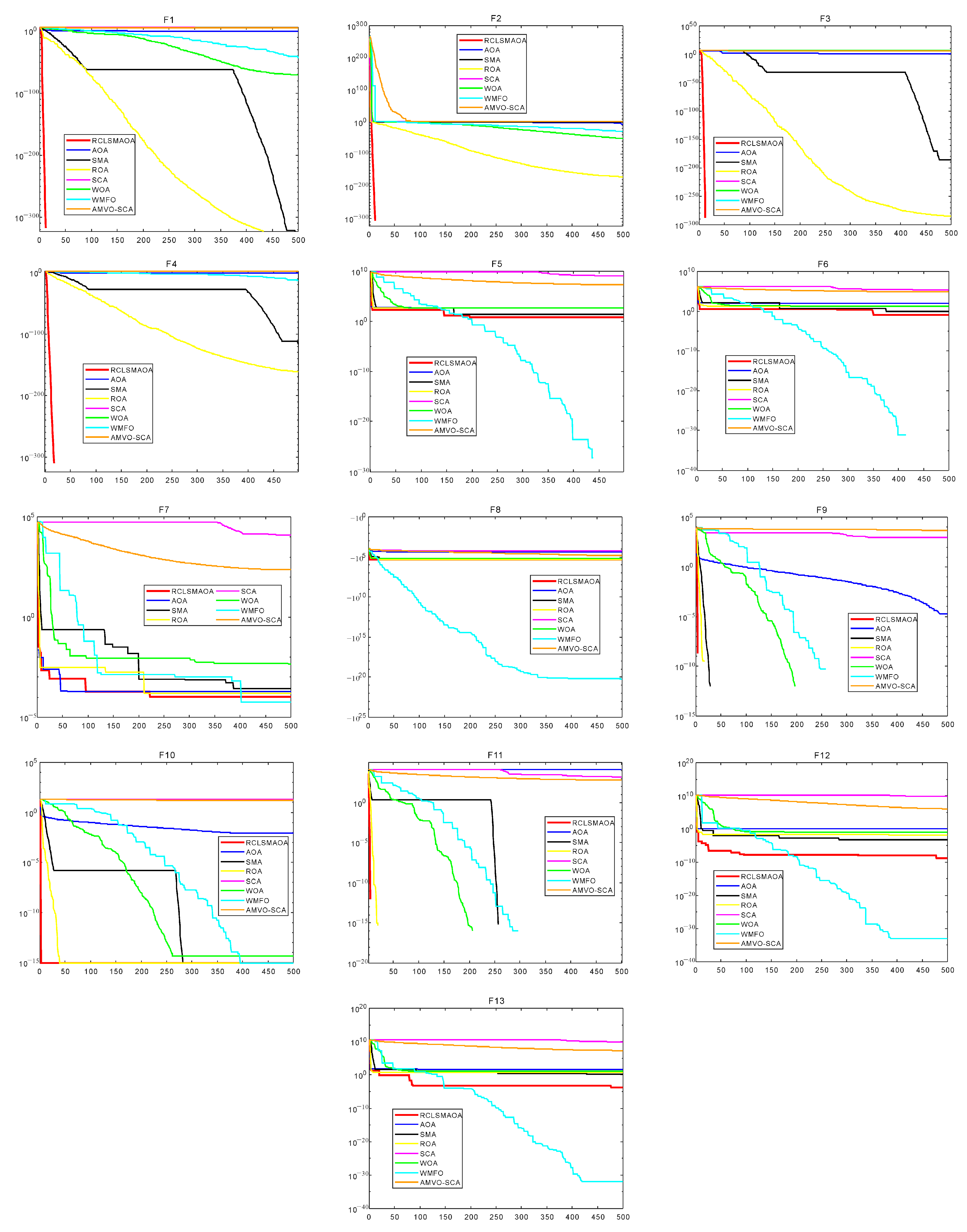
The specific experimental table is shown in Table 2, Table 3 and Table 4. We can see that on F1–F7, RCLSMAOA obtained the optimal values among three data items, including the optimal fitness value. We observed that the AOA performed well on F2, whereas the SMA performed well on F1 and F3. The RCLSMAOA inherits its advantages in single-mode functions. On the 500 dimensional scales, the RCLSMAOA still performs well. This is because mutation strategies can perform local mutations and increase global exploration capabilities.
Table 2.
Results of benchmark functions (F1–F13) under 30 dimensions.
Table 3.
Results of benchmark functions (F1–F13) under 500 dimensions.
Table 4.
Results of benchmark functions (F14–F23).
Similarly, we observed multimodal functions such as F8–F13. On F8, the optimal fitness value and the average value of RCLSMAOA reached the optimal value, and the standard deviation was slightly lower than that of SMA. Functions such as F9–F11 are relatively simple, giving most optimization algorithms good results. The performance of RCLSMAOA in the F12–13 function is also satisfactory. We observed that the performance of the RCLSMAOA will not be affected by changes in dimensions, and its performance remains stable. Functions such as F14–23 are fixed multimodal functions, which are relatively simple. In our experiment, it is not difficult to see that the performance of RCLSMAOA is still the best among the comparison algorithms. Although fixed multimodal functions are relatively simple, their performance in verifying algorithm performance is still reliable. The above analysis indicates that RCLSMAOA, which integrates SMA and AOA, performs better than SMA and AOA.
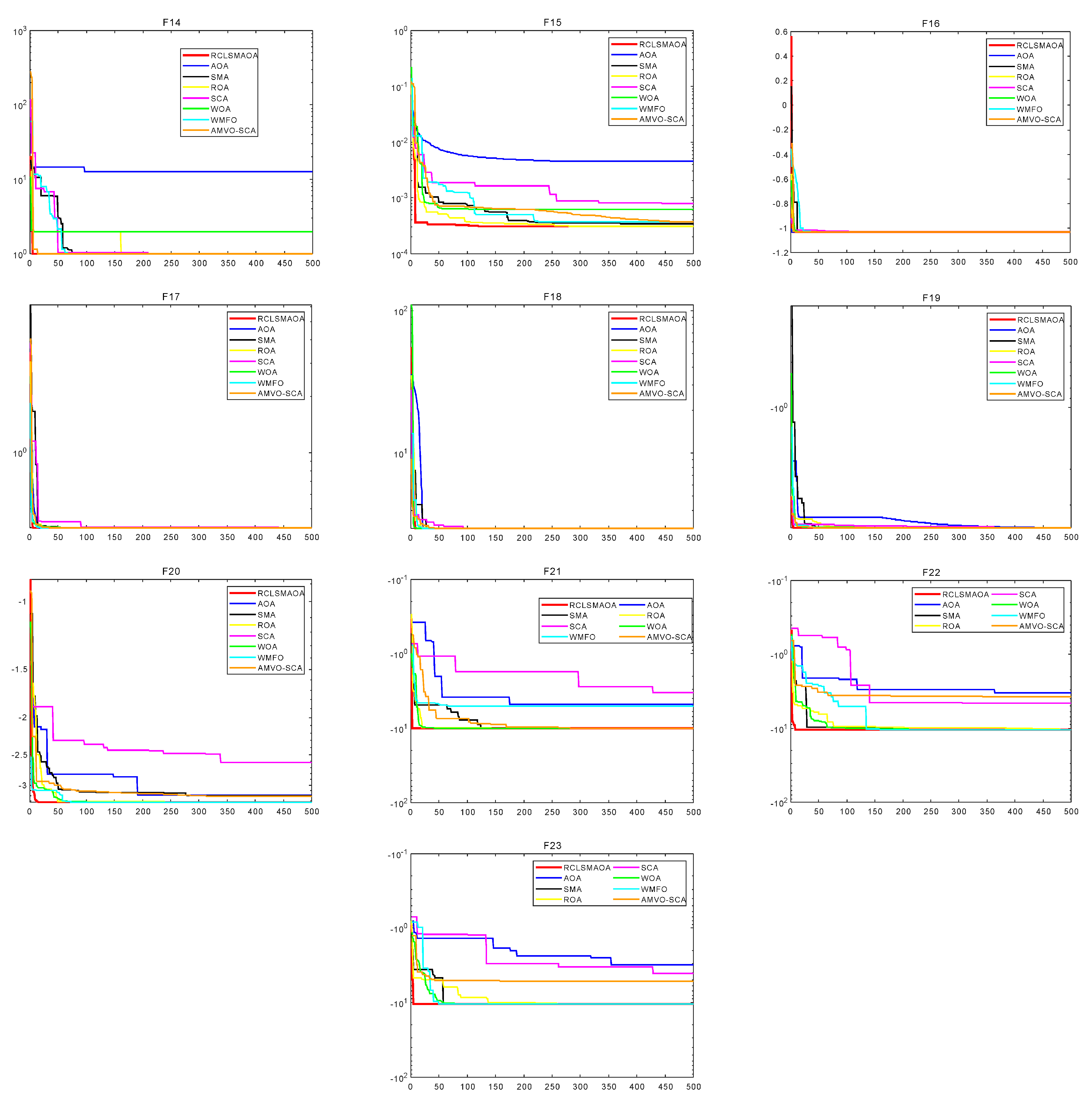
The data cannot intuitively understand the actual performance of the algorithm so we will show the convergence curves of each algorithm on F23 function images. The function image is shown in Figure 3, Figure 4 and Figure 5. From the image, we can see that in F1–F4, the RCLSMAOA has a fast convergence rate and high convergence precision, which SMA and AOA do not possess. This is due to the random center learning strategy, which expands the algorithm’s search range and enhances the convergence rate. For F5–6, RCLSMAOA can find a good position at the beginning of the iteration and then slowly converge to find the optimal position. Except for the WMFO algorithm, other algorithms stagnate in the early stages of the algorithm. For F7, the optimization ability of this algorithm is also stronger than other algorithms, because the existence of a restart strategy enables the algorithm to continuously jump out of local optima. On F8, the performance of RCLSMAOA is not as good as the WMFO algorithm, but stronger than other algorithms. F9–F11 is relatively simple and easy to find the optimal fitness value. RCLSMAOA algorithm is also the algorithm with the fastest rate of convergence. For F12–F13, the RCLSMAOA performs well and can also converge when other algorithms fall into local optima. F14–23 is a relatively simple function, but it can also play a role in verifying algorithm performance. On these functions, RCLSMAOA also always finds the optimal value the fastest. In summary, the RCLSMAOA applies to F23 functions.
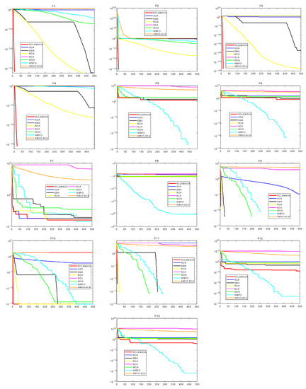
Figure 4.
F23 function images with dim = 500 (F1–F13).
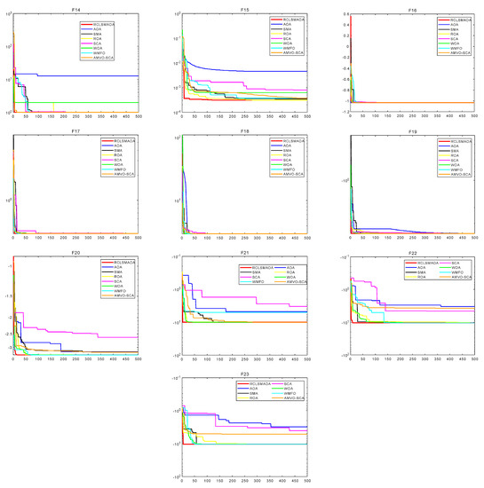
Figure 5.
F23 function images (F14–F23).
7.2. Experiments on the CEC2020 Benchmark Function
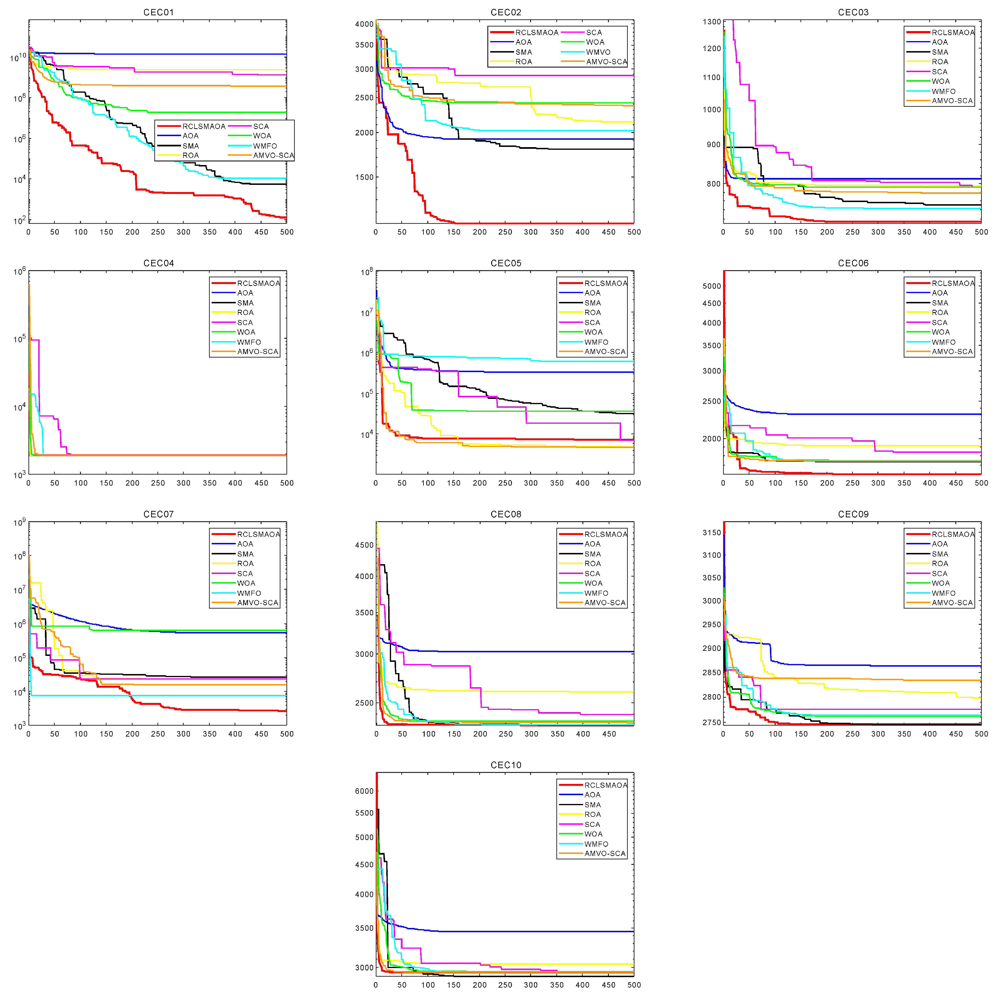
Using F23 functions for validation is not sufficient. We have added the CEC2020 test function [9] to verify this. In this experiment, we set the variables as N = 30, T = 500, and dim = 10. The comparison algorithm remains unchanged. The results of 30 runs of RCLSMAOA and other algorithms are shown in Table 5.
Table 5.
Results of benchmark functions (F14–F23).
CEC2020 has four class functions: unimodal function CEC01, basic multimodal function CEC02−4, mixed function CEC05-6, and combination function CEC06-10. In unimodal functions, the best one is RCLSMAOA, followed by SMA. This is because the RCLSMAOA integrates the SMA and adds mutation strategies to enhance its exploitation capabilities, enabling it to find better locations. The RCLSMAOA always performs stably based on multimodal functions and can find better values. This is based on the fact that the random center-solving strategy can effectively maintain a balance between exploration and exploitation in RCLSMAOA. Combined with the search strategy in SMA, the RCLSMAOA performs well on the basic multimodal functions. Mixed and combined functions are relatively difficult and complex and can easily trap functions into local optima. For this reason, we introduce a restart strategy to enable the RCLSMAOA to jump out of local optima. From the implementation results, the RCLSMAOA performs well and is not troubled by local optima.
To test the actual performance of the algorithm more clearly, we selected the specific convergence curves of the RCLSMAOA and other comparative algorithms, as shown in Figure 5. The convergence curves of the RLCSMAOA are mainly divided into two types. One is mainly reflected in the single-mode function. The RCLSMAOA can converge towards the optimal value and finally find the optimal value. This is because the RCLSMAOA integrates the position update formula from the SMA and uses a mutation strategy to improve it. Another is mainly reflected in the complex combination function and mixed function. To test the actual performance of the algorithm more clearly, we selected the specific convergence curves of the RCLSMAOA and other comparative algorithms, as shown in Figure 6. The convergence curves of the RLCSMAOA are mainly divided into two types. One is mainly reflected in the single-mode function. The RCLSMAOA can converge toward the optimal value and finally find the optimal value. This is because the RCLSMAOA integrates the position update formula from the SMA and uses a mutation strategy to improve it. Another is mainly reflected in the complex combination function and mixed function. For complex functions, RCLSMAOA shows a very fast convergence rate at the early stage of iteration. This is because RCLSMAOA uses the multiplication and division operator in the AOA, which allows the RCLSMAOA to find the optimal value very quickly.
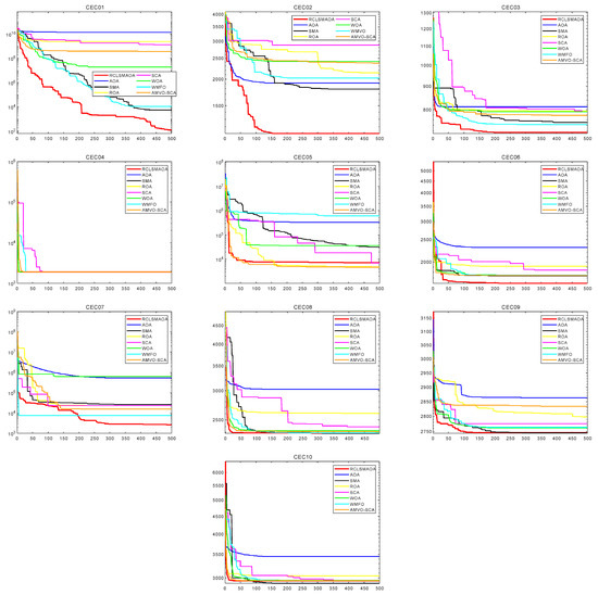
Figure 6.
Specific function image of CEC2020 test function.
7.3. Analysis of Wilcoxon Rank Sum Test Results and Friedman Test
Wilcoxon Rank Sum Test Results is a non-parametric detection test method that does not require any assumptions to be made about the data. Therefore, it applies to various types of data, including discrete, continuous, normal, and non-normal distribution. In this experiment, it was used to test whether two samples have differences. The experimental result of this experiment is p, when p is less than 5%. We believe there is a significant difference in the experimental results. Because the RCLSMAOA cannot compare with itself, we will not list the specific p-values of RCLSMAOA. Therefore, this article takes eight algorithms as samples; each algorithm independently solves 30 times and sets the population size N = 30. Among them, the dimensions selected for testing 23 standard test functions are 30 dimensions, and CEC2020 is ten dimensions.
Table 6 shows the experimental results of thirty experiments conducted on 23 standard test functions. Table 6 shows the experimental results of 30 experiments conducted on 23 standard test functions. For F1–F4, because the RCLSMAOA is a hybrid form of SMA, they are not distinguished in some functions. For F7–F11, these functions are simple, and most algorithms can achieve good results on them.
Table 6.
Experimental results of Wilcoxon rank sum test for F23 functions.
Table 7 shows the experimental results of thirty experiments conducted on the CEC2020 test function. We observed significant differences between the RCLSMAOA and other algorithms, except for CEC04. The main reason is that CEC04 is relatively simple compared to other functions, and most functions can find the optimal value.
Table 7.
Experimental results of Wilcoxon rank sum test for CEC2020 functions.
To verify the ranking of the algorithm, we used Friedman detection. We ran each algorithm independently 30 times to take the average value, and the results are shown in Table 8 and Table 9. The dimension chosen for F23 functions here is 30. It can be noted that RCLSMAOA is still in the first position.
Table 8.
Friedman ranked F23 functions.
Table 9.
Friedman ranked CEC2020 functions.
In this section, we conducted a more comprehensive data analysis of the algorithm’s performance using the Wilcoxon rank sum test and Friedman detection. We conclude that there are significant differences and good performance between the RCLSMAOA and most comparison algorithms for functions.
8. Engineering Issues
In this section, we will test the application of the RCLSMAOA in practical engineering problems in order to assess the quality and computational performance of RCLSMAOA in solving engineering problems and to explore whether it can achieve satisfactory results. This section will use five classic engineering problems to test the actual performance of the algorithm and compare it with other well-known optimization algorithms.
8.1. Pressure Vessel Design Problem
In practical survival problems, a common problem is pressure vessels. This issue aims to minimize the total cost of materials, forming, and welding for cylindrical containers. The structural schematic diagram is shown in Figure 7. This problem has four variables: shell thickness Ts, head thickness Th, internal radius R, and cylindrical section length L without considering the head.
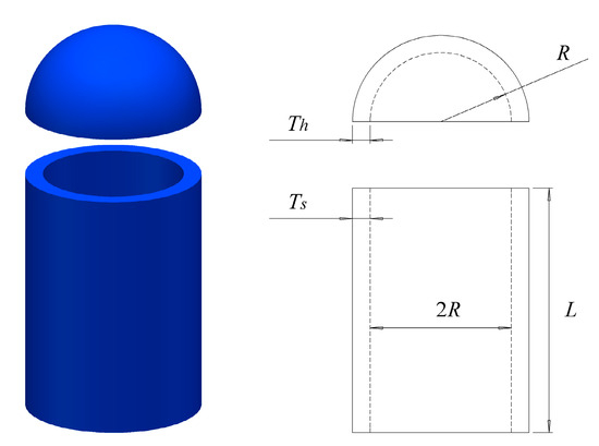
Figure 7.
The pressure vessel design.
The mathematical model of the pressure vessel design problem is as follows:
Consider:
Objective function:
Subject to:
Boundaries:
We can observe Table 10 to see the specific data of the RCLSMAOA on pressure vessel engineering issues. RCLSMAOA has Ts = 0.742433, Th = 0.370196, R = 40.31961, L = 200, COST = 5734.9131. Compared with other comparative algorithms, RCLSMAOA achieved the best results and achieved the optimal value of 200 on L. This means that RCLSMAOA can solve the engineering problem.
Table 10.
Comparison of optimal solutions for the pressure vessel design problem.
8.2. Speed Reducer Design Problem
The reducer is one of the key parts of the gearbox. In this study, we aim to achieve the minimum quality while meeting four design constraints and seven variables. The model structure is shown in Figure 8.
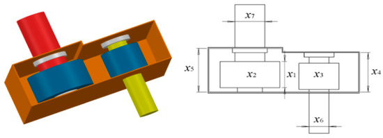
Figure 8.
Model of speed reducer design.
The mathematical model of reducer design is as follows:
Objective function:
Subject to:
Boundaries:
Table 11 shows that when x = [3.4975, 0.7, 17, 7.3, 7.8, 3.3500, 5.285], the minimum weight obtained by RCLSMAOA is 2995.437365, ranking first in the comparison algorithm. Observing experimental data, it can be seen that RCLSMAOA still performs well in relatively complex engineering problems.
Table 11.
Comparison of optimal solutions for the speed reducer design problem.
8.3. Three-Bar Truss Design Problem
In the design problem of a three-bar truss, in order to minimize the weight constrained by stress, deflection, and buckling, it is necessary to operate on two-bar lengths to minimize volume while satisfying the three constraint conditions. It has two decision variables, namely the lengths A1 and A2 of the two rods, and its specific physical model is shown in Figure 9.
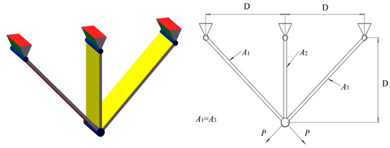
Figure 9.
Pressure vessel design problem.
The mathematical formulation of this problem is shown below:
Consider:
Minimize:
Subject to:
Variable Range:
The comparison results between RCLSMAOA and other algorithms in the design of three bar trusses are shown in Table 12. We observed that the data in the table are very close, indicating that it is difficult to optimize the problem better, but RCLSMAOA still achieved the best results.
Table 12.
Experimental results of three-bar truss design.
8.4. Welded Beam Design Problem
The welded beam design problem is a classic structural optimization problem and an important example in structural mechanics. This problem aims to minimize the steel plate’s total weight while satisfying four design variables of the connecting beam: thickness b, length L, height t, and width h. The detailed diagram of the welded beam is shown in Figure 10.
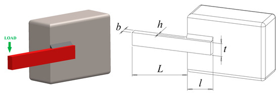
Figure 10.
Model of welded beams design.
The mathematical model of welded beam design is as follows:
Consider:
Objective function:
Subject to:
where:
Boundaries:
The specific data are shown in Table 13. The same RCLSMAOA still performs well in engineering problems, and the weight of the welded beam also reaches the minimum value. The results indicate that the IBWO algorithm is reliable for solving the problem of welded beams.
Table 13.
Comparison of optimal solutions for the welded beam design problem.
8.5. Car Crashworthiness Design Problem
The engineering issue refers to the safety performance of vehicles in a collision. This issue involves many aspects, including body structure, interior devices, and airbag systems. The car crashworthiness design problem is a very important issue in automotive design, which is directly related to the safety of passengers. The specific image is shown in Figure 11.
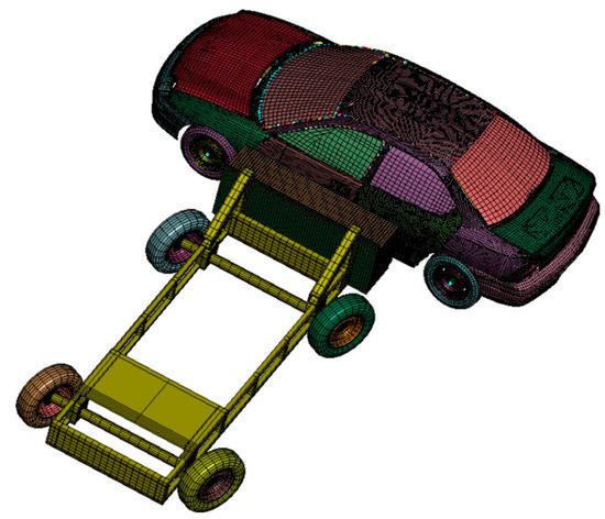
Figure 11.
Car crashworthiness design.
The mathematical formulation of this problem is shown below:
Minimize:
Subject to:
Variable Range:
The results of this engineering problem are shown in Table 14. In RCLSMAOA, X1, X3, X5, and X7 were all taken to the minimum value of 0.5, and the final weight was also the optimal value. This engineering problem shows that the RCLSMAOA still performs well in engineering problems with multiple variables and constraints.
Table 14.
Experimental results of car crashworthiness design.
9. Conclusions
This article fully considers the advantages and disadvantages of SMA and AOA optimization algorithms. It proposes a hybrid algorithm of slime mold and arithmetic optimization algorithm based on random center learning and restart mutation (RCLSMAOA). RCLSMAOA integrates the global search strategies of two algorithms. On this basis, a random center solution strategy is added to enhance the randomness of the algorithm, the effectiveness of global search, and the diversity of the algorithm population. The mutation strategy can enhance the convergence ability of the algorithm and further avoid the stagnation of the algorithm. Species reintroduction restart strategy can effectively avoid local optimization. The collaborative use of these strategies can help the RCLSMAOA enhance its optimization ability and maintain a good relationship between exploration and exploitation. In addition, we used the Wilcoxon rank sum test to test the significant differences between algorithms and achieved good results. Finally, five engineering experiments were conducted, and the RCLSMAOA provided an excellent solution.
From the experimental performance, convergence curve, and engineering problems, we can conclude that:
The RCLSMAOA proposed in this article combines the advantages of the SMA and AOA and effectively avoids the shortcomings of the two algorithms.
The newly proposed random center solution strategy can effectively address the shortcomings of RCLSMAOA and significantly enhance the algorithm’s global search ability.
The restart mutation strategy can improve the algorithm’s ability to overcome local optima and enhance the balance between exploration and exploitation.
By verifying the results of different test functions, the actual performance of the RCLSMAOA was effectively tested
Finally, by verifying five engineering problems, it can be concluded that the RCLSMAOA has good engineering application prospects.
This paper only studies the fusion of two optimization algorithms and adds three effective strategies. RCMSMAOA is still prone to local optimality in high dimensional space, and the convergence accuracy is not enough, and in some engineering problems did not show obvious advantages. In the future, we will further improve the performance of RCLSMAOA in practical engineering problems and improve the applicability of this algorithm in high-dimensional space. In future work, we will study the binary version of RCLSMAOA and use it to solve the feature selection problem.
Author Contributions
Conceptualization, Z.W. and H.C.; Methodology, H.J.; Software, H.C. and H.J.; Validation, H.J. and X.Z.; Formal analysis, H.C., H.J. and X.Z.; Investigation, H.C. and H.J.; Code, Z.W.; Resources, H.C. and Z.W.; Data Management, H.J. and L.A.; Writing—drafting the first draft, H.C. and Z.W.; Writing—Review and Editing, H.J. and H.C.; Visualization, Z.W., H.C. and X.Z.; Supervision, H.C. and H.J.; funding acquisition, H.C. and H.J. All authors have read and agreed to the published version of the manuscript.
Funding
This research was funded by the Ministry of Education National Education Science Planning Key Project—“Collaborative Edu-cation Project of the Ministry of Education” [grant number 202102391036], a Natural Science Foundation of Fujian Province of China [grant number 2023J011030], a Middle-aged and Young Teachers’ Education and Research Project of Fujian Province [grant number JAT210423], a Sanming College Scientific Research and Development Fund Grant [grant number B202104], a Fuzhou City Science and Technology Plan Project [grant number 2021-P-064] and the APC was funded by the Tianjin Municipal Health and Health Committee.
Institutional Review Board Statement
Not applicable.
Data Availability Statement
Not applicable.
Acknowledgments
This work is supported by Fujian Key Lab of Agriculture IOT Application, and IOT Application Engineering Research Center of Fujian Province Colleges and Universities.
Conflicts of Interest
The authors declare no conflict of interest.
References
- Pierezan, J.; Coelho, L.D.S. Coyote Optimization Algorithm: A New Metaheuristic for Global Optimization Problems. In Proceedings of the 2018 IEEE Congress on Evolutionary Computation (CEC), Rio de Janeiro, Brazil, 8–13 July 2018. [Google Scholar] [CrossRef]
- Dhiman, G.; Kumar, V. Emperor penguin optimizer: A bio-inspired algorithm for engineering problems. Knowl. Based Syst. 2018, 159, 20–50. [Google Scholar] [CrossRef]
- Malviya, R.; Pratihar, D.K. Tuning of neural networks using particle swarm optimization to model MIG welding process. Swarm Evol. Comput. 2011, 1, 223–235. [Google Scholar] [CrossRef]
- Nanda, S.J.; Panda, G. A survey on nature inspired methaheuristic algorithms for partitional clustering. Swarm Evol. Comput. 2014, 16, 1–18. [Google Scholar] [CrossRef]
- Changdar, C.; Mahapatra, G.; Pal, R.K. An efficient genetic algorithm for multi-objective solid travelling salesman problem under fuzziness. Swarm Evol. Comput. 2014, 15, 27–37. [Google Scholar] [CrossRef]
- Suresh, K.; Kumarappan, N. Hybrid improved binary particle swarm optimization approach for generation maintenance scheduling problem. Swarm Evol. Comput. 2012, 9, 69–89. [Google Scholar] [CrossRef]
- Beyer, H.G.F.; Schwefel, H.P. Evolution strategies-a comprehensive introduction. Nat. Comput. 2002, 1, 3–52. [Google Scholar] [CrossRef]
- Chen, H.; Wang, Z.; Wu, D.; Jia, H.; Wen, C.; Rao, H.; Abualigah, L. An improved multi-strategy beluga whale optimization for global optimization problems. Math. Biosci. Eng. 2023, 20, 13267–13317. [Google Scholar] [CrossRef]
- Wen, C.; Jia, H.; Wu, D.; Rao, H.; Li, S.; Liu, Q.; Abualigah, L. Modified Remora Optimization Algorithm with Multistrategies for Global Optimization Problem. Mathematics 2022, 10, 3604. [Google Scholar] [CrossRef]
- Wu, D.; Rao, H.; Wen, C.; Jia, H.; Liu, Q.; Abualigah, L. Modified Sand Cat Swarm Optimization Algorithm for Solving Constrained Engineering Optimization Problems. Mathematics 2022, 10, 4350. [Google Scholar] [CrossRef]
- Abualigah, L.; Diabat, A.; Mirjalili, S.; Elaziz, M.A.; Gandomi, A.H. The arithmetic optimization algorithm. Comput. Methods Appl. Mech. Eng. 2021, 376, 113609. [Google Scholar] [CrossRef]
- Wang, R.-B.; Wang, W.-F.; Xu, L.; Pan, J.-S.; Chu, S.-C. An Adaptive Parallel Arithmetic Optimization Algorithm for Robot Path Planning. J. Adv. Transp. 2021, 2021, 3606895. [Google Scholar] [CrossRef]
- Khodadadi, N.; Snasel, V.; Mirjalili, S. Dynamic Arithmetic Optimization Algorithm for Truss Optimization Under Natural Frequency Constraints. IEEE Access 2022, 10, 16188–16208. [Google Scholar] [CrossRef]
- Li, X.-D.; Wang, J.-S.; Hao, W.-K.; Zhang, M.; Wang, M. Chaotic arithmetic optimization algorithm. Appl. Intell. 2022, 52, 16718–16757. [Google Scholar] [CrossRef]
- Li, S.; Chen, H.; Wang, M.; Heidari, A.A.; Mirjalili, S. Slime mould algorithm: A new method for stochastic optimization. Future Gener. Comput. Syst. 2020, 111, 300–323. [Google Scholar] [CrossRef]
- Kouadri, R.; Musirin, I.; Slimani, L.; Bouktir, T.; Othman, M. Optimal powerflow control variables using slime mould algorithm forgenerator fuel cost and loss minimization with voltage profileenhancement solution. Int. J. EmergingTrends Eng. Res. 2020, 8, 36–44. [Google Scholar]
- Zhao, J.; Gao, Z.M. The hybridized Harris hawk optimizationand slime mould algorithm. J. Phys. Conf. Ser. 2020, 1682, 012029. [Google Scholar] [CrossRef]
- Rashedi, E.; Nezamabadi-Pour, H.; Saryazdi, S. GSA: A Gravitational Search Algorithm. Inf. Sci. 2009, 179, 2232–2248. [Google Scholar] [CrossRef]
- Hatamlou, A. Black hole: A new heuristic optimization approach for data clustering. Inf. Sci. 2013, 222, 175–184. [Google Scholar] [CrossRef]
- Kirkpatrick, S.; Gelatto, C.D.; Vecchi, M.P. Optimization by simulated annealing. Science 1983, 220, 671–680. [Google Scholar] [CrossRef]
- Holland, J.H. Genetic algorithms. Sci. Am. 1992, 267, 66–73. [Google Scholar] [CrossRef]
- Banzhaf, W.; Nordin, P.; Keller, R.E.; Francone, F.D. Genetic Programming: An Introduction; Morgan Kaufmann Publishers: San Francisco, CA, USA, 1998; Volume 1. [Google Scholar]
- Storn, R.; Price, K. Differential evolution—A simple and efficient heuristic for global optimization over continuous spaces. J. Glob. Optim. 1997, 11, 341–359. [Google Scholar] [CrossRef]
- Kennedy, J.; Eberhart, R. Particle swarm optimization. In Proceedings of the ICNN’95—International Conference on Neural Networks, Perth, WA, Australia, 27 November–1 December 1995; Volume 4, pp. 1942–1948. [Google Scholar]
- Dorigo, M.; Maniezzo, V.; Colorni, A. Ant system: Optimization by a colony of cooperating agents. IEEE Trans. Syst. Man Cybern. Part B Cybern. 1996, 26, 29–41. [Google Scholar] [CrossRef]
- Rao, R.V.; Savsani, V.J.; Vakharia, D.P. Teaching–learning-based optimization: A novel method for constrained mechanical design optimization problems. Comput. Aided Des. 2011, 43, 303–315. [Google Scholar] [CrossRef]
- Dehghani, M.; Trojovská, E.; Trojovský, P. A new human-based metaheuristic algorithm for solving optimization problems on the base of simulation of driving training process. Sci. Rep. 2022, 12, 9924. [Google Scholar] [CrossRef]
- Gandomi, A.H. Interior search algorithm (ISA): A novel approach for global optimization. ISA Trans. 2014, 53, 1168–1183. [Google Scholar] [CrossRef] [PubMed]
- Wang, G.G.; Deb, S.; Cui, Z. Monarch butterfly optimization. Neural Comput. Appl. 2019, 31, 1995–2014. [Google Scholar] [CrossRef]
- Wang, G.G. Moth search algorithm: A bio-inspired metaheuristic algorithm for global optimization problems. Memetic Comput. 2018, 10, 151–164. [Google Scholar] [CrossRef]
- Yang, Y.; Chen, H.; Heidari, A.A.; Gandomi, A.H. Hunger games search: Visions, conception, implementation, deep analysis, perspectives, and towards performance shifts. Expert Syst. Appl. 2021, 177, 114864. [Google Scholar] [CrossRef]
- Ahmadianfar, I.; Heidari, A.A.; Gandomi, A.H.; Chu, X.; Chen, H. RUN beyond the metaphor: An efficient optimization algorithm based on Runge Kutta method. Expert Syst. Appl. 2021, 181, 115079. [Google Scholar] [CrossRef]
- Tu, J.; Chen, H.; Wang, M.; Gandomi, A.H. The colony predation algorithm. J. Bionic Eng. 2021, 18, 674–710. [Google Scholar] [CrossRef]
- Ahmadianfar, I.; Heidari, A.A.; Noshadian, S.; Chen, H.; Gandomi, A.H. INFO: An efficient optimization algorithm based on weighted mean of vectors. Expert Syst. Appl. 2022, 195, 116516. [Google Scholar] [CrossRef]
- Heidari, A.A.; Mirjalili, S.; Faris, H.; Aljarah, I.; Mafarja, M.; Chen, H. Harris hawks optimization: Algorithm and applications. Future Gener. Comput. Syst. 2019, 97, 849–872. [Google Scholar] [CrossRef]
- Su, H.; Zhao, D.; Heidari, A.A.; Liu, L.; Zhang, X.; Mafarja, M.; Chen, H. RIME: A physics-based optimization. Neurocomputing 2023, 532, 183–214. [Google Scholar] [CrossRef]
- Zeb, A.; Khan, M.; Khan, N.; Tariq, A.; Ali, L.; Azam, F.; Jaffery, S.H.I. Hybridization of simulated annealing with genetic algorithm for cell formation problem. Int. J. Adv. Manuf. Technol. 2016, 86, 2243–2254. [Google Scholar] [CrossRef]
- Chen, Z.; Chen, R.; Deng, T.; Wang, Y.; Di, W.; Luo, H.; Han, T. Magnetic Anomaly Detection Using Three-Axis Magnetoelectric Sensors Based on the Hybridization of Particle Swarm Optimization and Simulated Annealing Algorithm. IEEE Sensors J. 2021, 22, 3686–3694. [Google Scholar] [CrossRef]
- Nadimi-Shahraki, M.H.; Fatahi, A.; Zamani, H.; Mirjalili, S.; Oliva, D. Hybridizing of Whale and Moth-Flame Optimization Algorithms to Solve Diverse Scales of Optimal Power Flow Problem. Electronics 2022, 11, 831. [Google Scholar] [CrossRef]
- Mohd Tumari, M.Z.; Ahmad, M.A.; Suid, M.H.; Hao, M.R. An Improved Marine Predators Algorithm-Tuned Fractional-Order PID Controller for Automatic Voltage Regulator System. Fractal Fract. 2023, 7, 561. [Google Scholar] [CrossRef]
- Wang, L.; Shi, R.; Dong, J. A Hybridization of Dragonfly Algorithm Optimization and Angle Modulation Mechanism for 0-1 Knapsack Problems. Entropy 2021, 23, 598. [Google Scholar] [CrossRef]
- Devaraj AF, S.; Elhoseny, M.; Dhanasekaran, S.; Lydia, E.L.; Shankar, K. Hybridization of firefly and improved multi-objective particle swarm op-timization algorithm for energy efficient load balancing in cloud computing environments. J. Parallel Distrib. Comput. 2020, 142, 36–45. [Google Scholar] [CrossRef]
- Jui, J.J.; Ahmad, M.A. A hybrid metaheuristic algorithm for identification of continuous-time Hammerstein systems. Appl. Math. Model. 2021, 95, 339–360. [Google Scholar] [CrossRef]
- Zhang, H.; Wang, Z.; Chen, W.; Heidari, A.A.; Wang, M.; Zhao, X.; Liang, G.; Chen, H.; Zhang, X. Ensemble mutation-driven salp swarm algorithm with restart mechanism: Framework and fundamental analysis. Expert Syst. Appl. 2020, 165, 113897. [Google Scholar] [CrossRef]
- Jia, H.; Peng, X.; Lang, C. Remora optimization algorithm. Expert Syst. Appl. 2021, 185, 115665. [Google Scholar] [CrossRef]
- Mirjalili, S. SCA: A Sine Cosine Algorithm for solving optimization problems. Knowl.-Based Syst. 2016, 96, 120–133. [Google Scholar] [CrossRef]
- Mirjalili, S.; Lewis, A. The whale optimization algorithm. Adv. Eng. Softw. 2016, 95, 51–67. [Google Scholar] [CrossRef]
- Mirjalili, S.; Lewis, A. Grey Wolf Optimizer. Adv. Eng. Softw. 2014, 69, 46–61. [Google Scholar] [CrossRef]
- Dorigo, M.; Birattari, M.; Stutzle, T. Ant colony optimization. IEEE Comput. Intell. Mag 2006, 1, 28–39. [Google Scholar] [CrossRef]
- Abualigah, L.; Yousri, D.; Abd Elaziz, M.; Ewees, A.A.; Al-Qaness, M.A.; Gandomi, A.H. Aquila Optimizer: A novel meta-heuristic optimization algorithm. Comput. Ind. Eng. 2021, 157, 107250. [Google Scholar] [CrossRef]
- Mirjalili, S.; Mirjalili, S.M.; Hatamlou, A. Multi-verse optimizer: A nature-inspired algorithm for global optimization. Neural Comput. Appl. 2016, 27, 495–513. [Google Scholar] [CrossRef]
- Baykasoğlu, A.; Ozsoydan, F.B. Adaptive firefly algorithm with chaos for mechanical design optimization problems. Appl. Soft Comput. 2015, 36, 152–164. [Google Scholar] [CrossRef]
- Abualigah, L.; Abd Elaziz, M.; Sumari, P.; Geem, Z.W.; Gandomi, A.H. Reptile Search Algorithm (RSA): A nature-inspired meta-heuristic optimizer. Expert Syst. Appl. 2022, 191, 116158. [Google Scholar] [CrossRef]
- Mirjalili, S. Moth-flame optimization algorithm: A novel nature-inspired heuristic paradigm. Knowl. Based Syst. 2015, 89, 228–249. [Google Scholar] [CrossRef]
- Czerniak, M.; Zarzycki, H.; Ewald, D. AAO as a new strategy in modeling and simulation of constructional problems optimiza-tion. Simul. Modell. Pract. Theory 2017, 76, 22–33. [Google Scholar] [CrossRef]
- Geem, Z.W.; Kim, J.H.; Loganathan, G.V. A new heuristic optimization algorithm: Harmony search. Simulation 2001, 76, 60–68. [Google Scholar] [CrossRef]
- Baykasoglu, A.; Akpinar, S. Weighted superposition attraction (WSA): A swarm intelligence algorithm for optimization prob-lems-part2: Constrained optimization. Appl. Softw. Comput. 2015, 37, 396–415. [Google Scholar] [CrossRef]
- Gandomi, A.H.; Yang, X.-S.; Alavi, A.H. Cuckoo search algorithm: A metaheuristic approach to solve structural optimization problems. Eng. Comput. 2013, 29, 17–35. [Google Scholar] [CrossRef]
- Saremi, S.; Mirjalili, S.; Lewis, A. Grasshopper Optimisation Algorithm: Theory and application. Adv. Eng. Softw. 2017, 105, 30–47. [Google Scholar] [CrossRef]
- Rao, H.; Jia, H.; Wu, D.; Wen, C.; Li, S.; Liu, Q.; Abualigah, L. A Modified Group Teaching Optimization Algorithm for Solving Constrained Engineering Optimization Problems. Mathematics 2022, 10, 3765. [Google Scholar] [CrossRef]
- Kaveh, A.; Khayatazad, M. A new meta-heuristic method: Ray Optimization. Comput. Struct. 2012, 112–113, 283–294. [Google Scholar] [CrossRef]
- Zhong, C.; Li, G.; Meng, Z. Beluga whale optimization: A novel nature-inspired metaheuristic algorithm. Knowl. Based Syst. 2022, 251, 109215. [Google Scholar] [CrossRef]
- Wang, S.; Sun, K.; Zhang, W.; Jia, H. Multilevel thresholding using a modified ant lion optimizer with opposition-based learning for color image segmentation. Math. Biosci. Eng. 2021, 18, 3092–3143. [Google Scholar] [CrossRef]
- Zhang, Y.; Jin, Z. Group teaching optimization algorithm: A novel metaheuristic method for solving global optimization problems. Expert Syst. Appl. 2020, 148, 113246. [Google Scholar] [CrossRef]
- Houssein, E.H.; Neggaz, N.; Hosney, M.E.; Hosney, M.E.; Mohamed, W.M.; Hassaballah, M. Enhanced Harris hawks opti-mization with genetic operators for selection chemical descriptors and compounds activities. Neural Comput. Appl. 2021, 33, 13601–13618. [Google Scholar] [CrossRef]
- Long, W.; Jiao, J.; Liang, X.; Cai, S.; Xu, M. A Random Opposition-Based Learning Grey Wolf Optimizer. IEEE Access 2019, 7, 113810–113825. [Google Scholar] [CrossRef]
- Faramarzi, A.; Heidarinejad, M.; Mirjalili, S.; Gandomi, A.H. Marine Predators Algorithm: A nature-inspired metaheuristic. Expert Syst. Appl. 2020, 152, 113377. [Google Scholar] [CrossRef]


Disclaimer/Publisher’s Note: The statements, opinions and data contained in all publications are solely those of the individual author(s) and contributor(s) and not of MDPI and/or the editor(s). MDPI and/or the editor(s) disclaim responsibility for any injury to people or property resulting from any ideas, methods, instructions or products referred to in the content. |
© 2023 by the authors. Licensee MDPI, Basel, Switzerland. This article is an open access article distributed under the terms and conditions of the Creative Commons Attribution (CC BY) license (https://creativecommons.org/licenses/by/4.0/).