Rapidly Exploring Random Tree Algorithm-Based Path Planning for Worm-Like Robot


Abstract
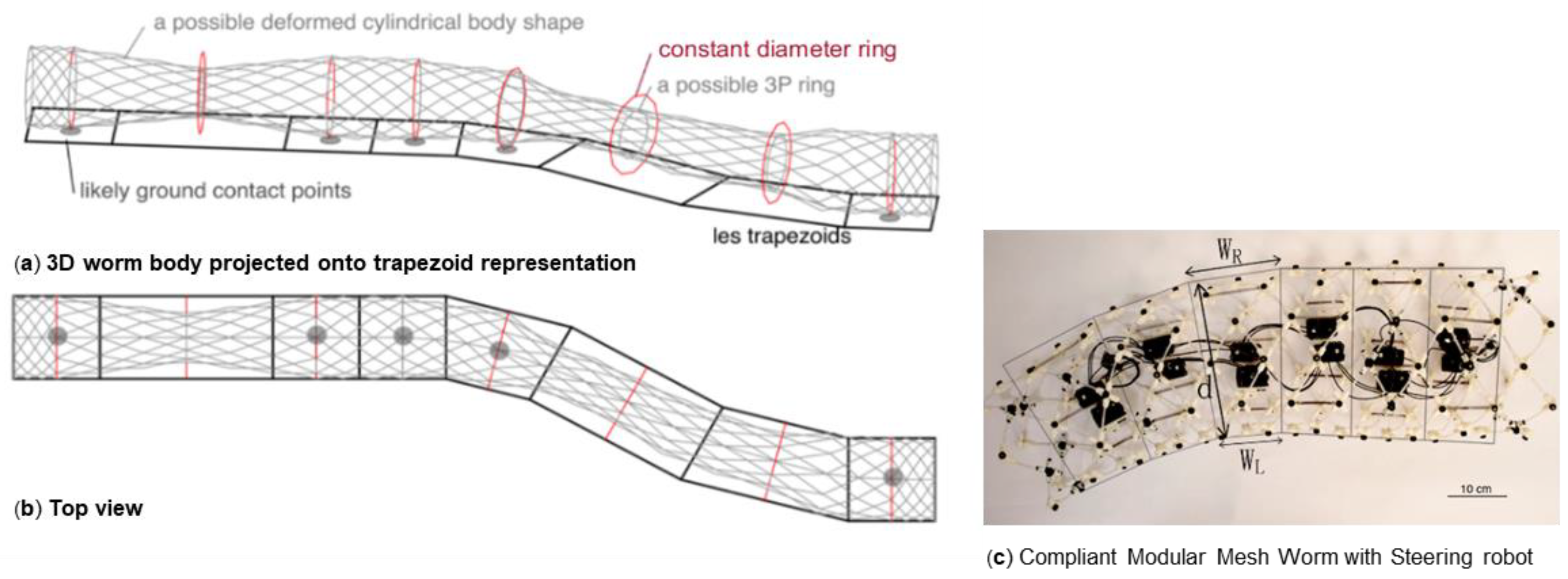
1. Introduction
Related Work
2. Methods: Pathfinding Algorithms
2.1. Random Trees (RRT)
| Algorithm 1 RRT |
| Input: Initial and desired configuration of the robot, the maximum number of samples, Nmax |
| Output: Tree, T |
|
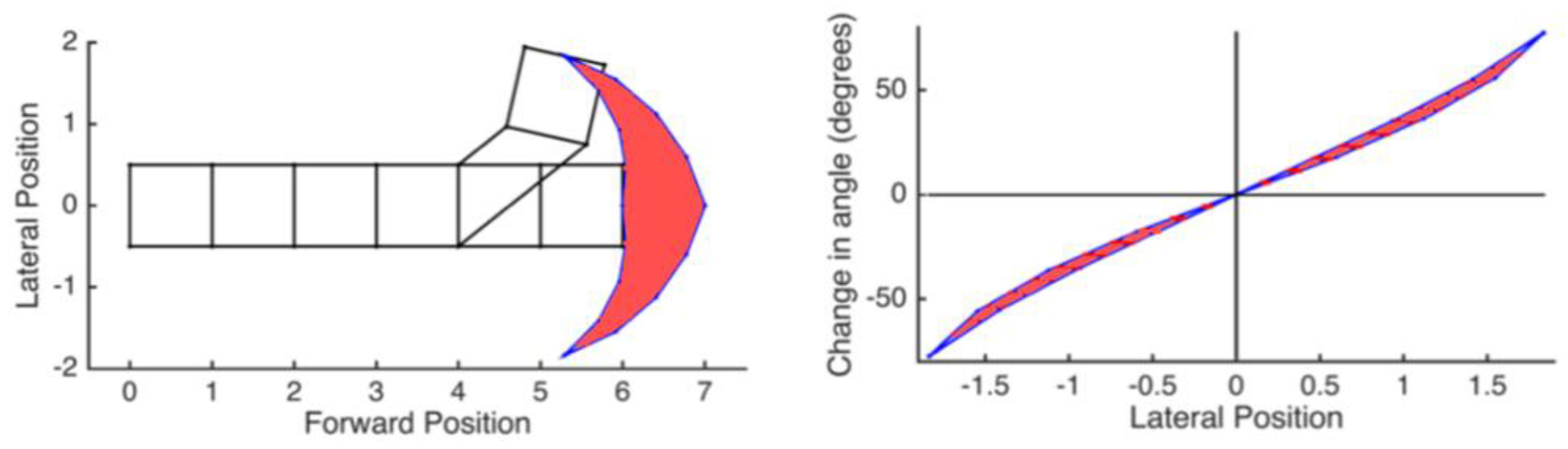
2.2. Elliptical Path Generation
- The robot is tangent to the curve at the start coordinate
- The robot is tangent to the curve at the goal coordinate
- The start coordinate of the head center of the robot satisfies the equation of the curve.
- The goal coordinate of the head center of the robot satisfies the equation of the curve.
| Algorithm 2 Elliptical path generation |
| Input: Initial and desired configuration of the robot |
| Output: List of angles, W |
|
| where (xr, yr) is the robot’s center coordinate of the head of initial configuration, mr is the robot’s tangent of the orientation of initial configuration and (xd, yd) is the center coordinate of the head of desired goal configuration, md is the tangent of the orientation of the desired configuration |
|
2.3. Combined RRT Ellipse
| Algorithm 3 Combined RRT and elliptical path |
| Input: Initial and desired configuration of the robot, the maximum number of samples, Nmax |
| Output: Tree, T |
| Add initial configuration to the tree, T |
|
|
| (xn,yn) is the coordinate of the head of Cs and θs is the tangent of the orientation of Cs |
|
|
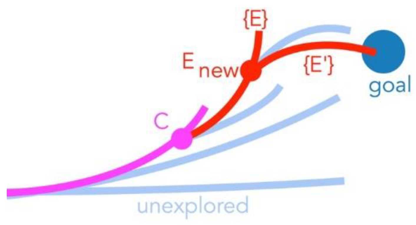
2.4. Enhanced Combined RRT Ellipse
| Algorithm 4 Enhanced combined RRT and elliptical path |
| Input: Initial and desired configuration of the robot, the maximum number of samples, Nmax |
| Output: Tree, T |
|
| Else: |
| Add Cnew to T |
|
3. Experimental Results
3.1. Rapidly Exploring Random Trees
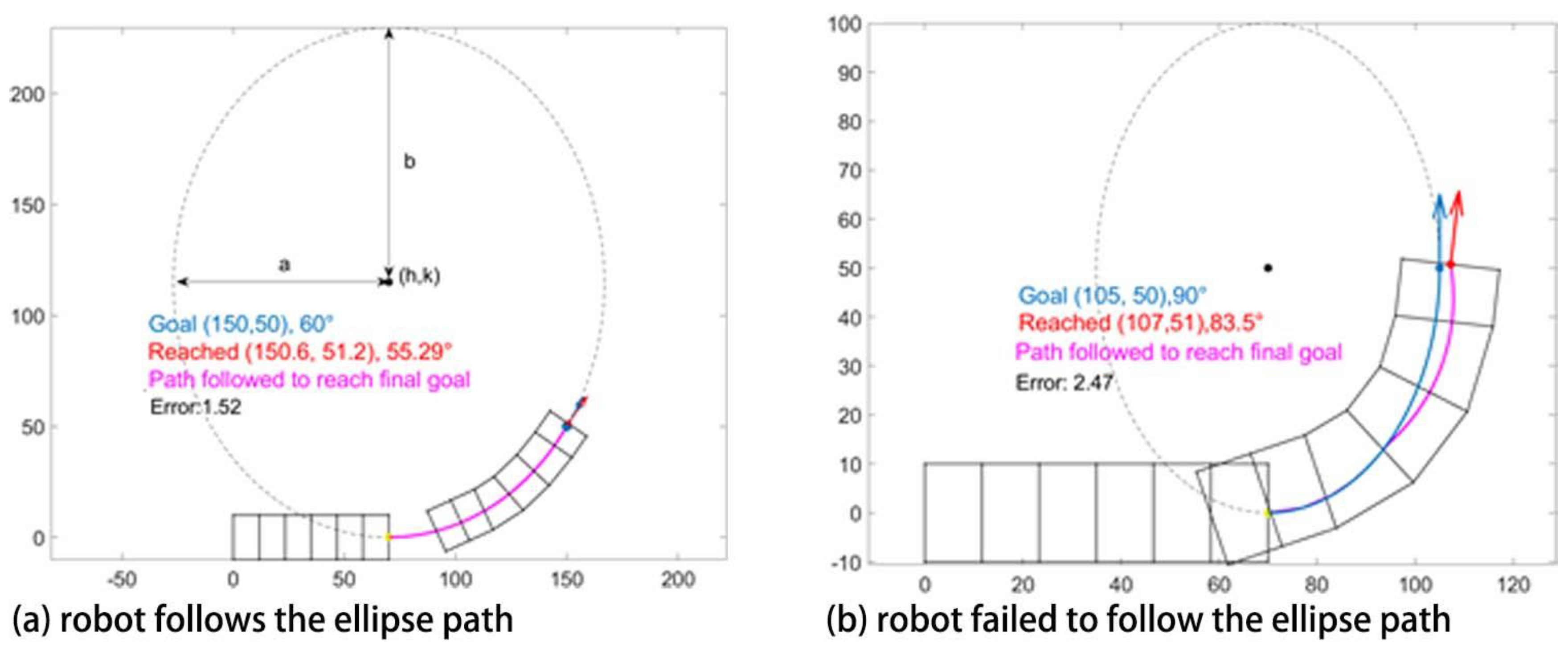
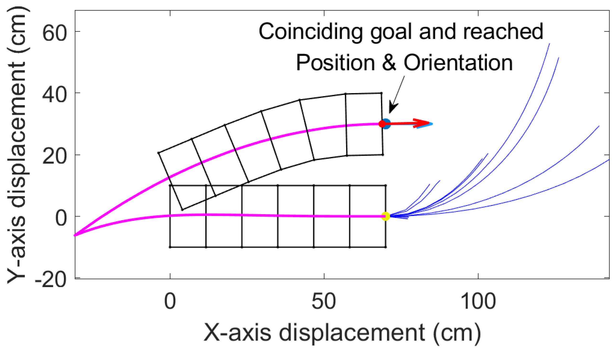
3.2. Elliptical Path Generation
3.3. Enhanced Combined RRT Ellipse
3.4. Enhanced Combined RRT Ellipse (ECRE)
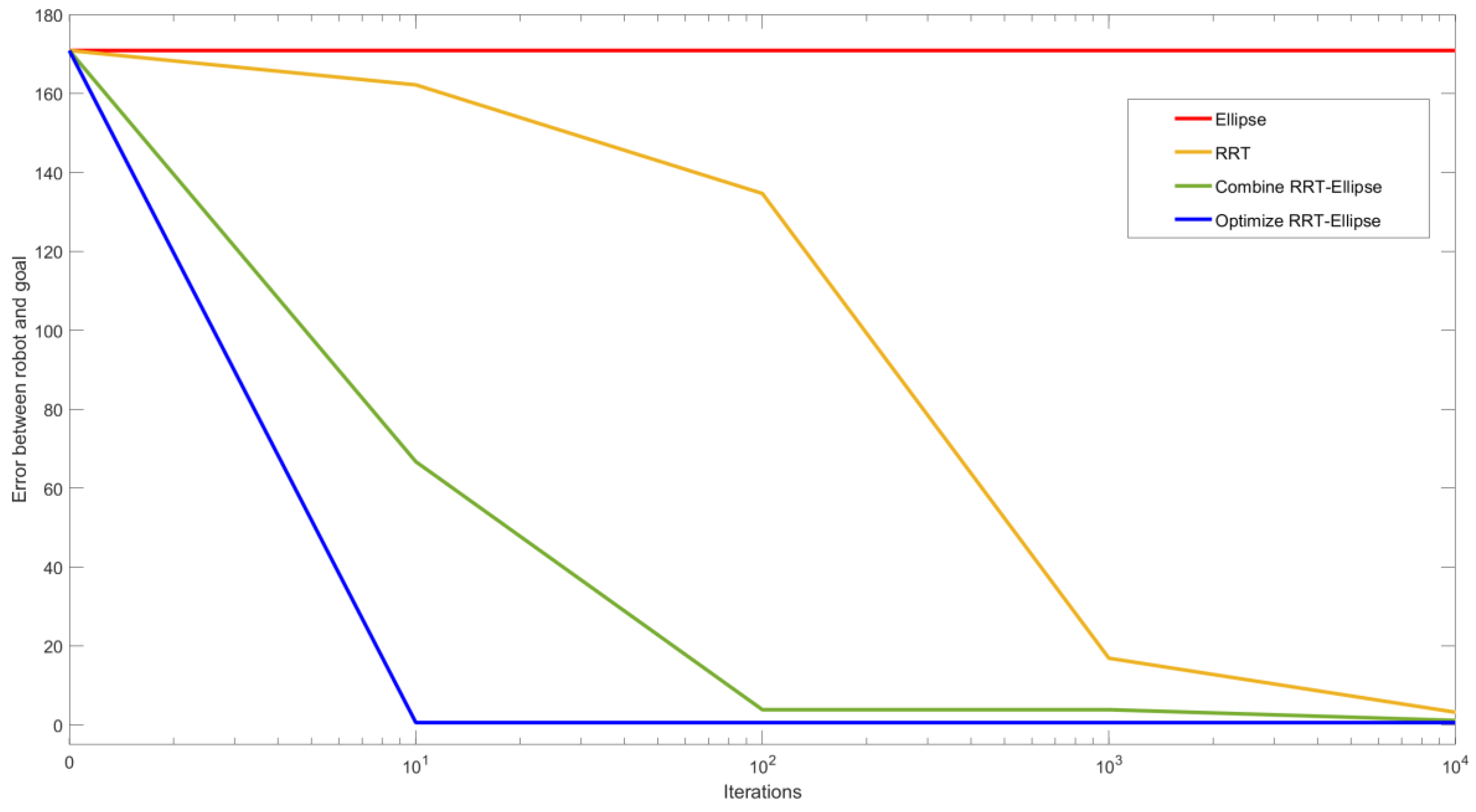
3.5. Algorithm Efficiency Comparison
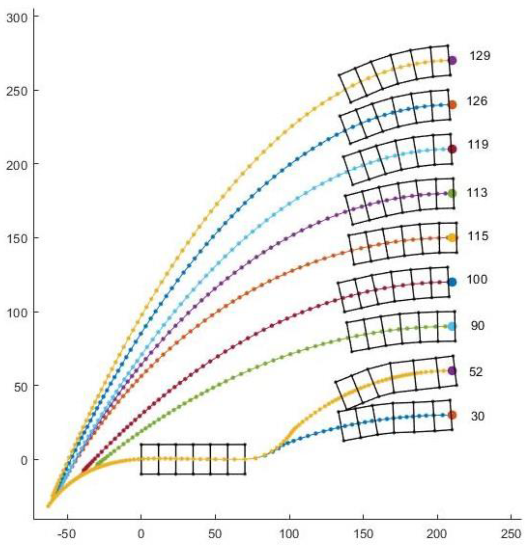
3.6. Path Analysis of Reachable Space
4. Discussion
5. Conclusions
Author Contributions
Funding
Conflicts of Interest
References
- Trivedi, D.; Rahn, C.D.; Kier, W.M.; Walker, I.D. Soft Robotics: Biological Inspiration, State of the Art, and Future Research. Appl. Bionics Biomech. 2008, 5, 99–117. [Google Scholar] [CrossRef]
- Polygerinos, P.; Correll, N.; Morin, S.A.; Mosadegh, B.; Onal, C.D.; Petersen, K.; Cianchetti, M.; Tolley, M.T.; Shepherd, R.F. Soft Robotics: Review of Fluid-Driven Intrinsically Soft Devices; Manufacturing, Sensing, Control, and Applications in Human-Robot Interaction. Adv. Eng. Mater. 2017, 19, 1700016. [Google Scholar] [CrossRef]
- Kandhari, A.; Wang, Y.; Daltorio, K.; Chiel, H.J. Turning in Worm-Like Robots: The Geometry of Slip Elimination Suggests Nonperiodic Waves. Soft Robot. 2019, 6, 560–577. [Google Scholar] [CrossRef] [PubMed]
- Horchler, A.D.; Kandhari, A.; Daltorio, K.A.; Moses, K.C.; Andersen, K.B.; Bunnelle, H.; Kershaw, J.; Tavel, W.H.; Bachmann, R.J.; Chiel, H.J.; et al. Worm-Like Robotic Locomotion with a Compliant Modular Mesh. In Biomimetic and Biohybrid Systems. Living Machines 2015; Lecture Notes in Computer Science; Wilson, S., Verschure, P., Mura, A., Prescott, T., Eds.; Springer: Berlin/Heidelberg, Germany, 2015; Volume 9222. [Google Scholar]
- Zhan, X.; Fang, H.; Xu, J.; Wang, K.-W. Planar locomotion of earthworm-like metameric robots. Int. J. Robot. Res. 2019, 38, 1751–1774. [Google Scholar] [CrossRef]
- Lavalle, S.M. Rapidly-Exploring Random Trees: A New Tool for Path Planning; Technical Report; Computer Science Department, Iowa State University: Ames, IA, USA, October 1998. [Google Scholar]
- González, D.; Pérez, J.; Milanés, V.; Nashashibi, F. A Review of Motion Planning Techniques for Automated Vehicles. IEEE Trans. Intell. Transp. Syst. 2016, 17, 1135–1145. [Google Scholar] [CrossRef]
- Scheuer, A.; Fraichard, T. Continuous-curvature path planning for car-like vehicles. In Proceedings of the 1997 IEEE/RSJ International Conference on Intelligent Robot and Systems. Innovative Robotics for Real-World Applications. IROS ‘97, Grenoble, France, 11 September 1997; Volume 2, pp. 997–1003. [Google Scholar]
- Yang, K.; Sukkarieh, S. An Analytical Continuous-Curvature Path-Smoothing Algorithm. IEEE Trans. Robot. 2010, 26, 561–568. [Google Scholar] [CrossRef]
- Liu, J.; Wang, Y.; Ii, B.; Ma, S. Path planning of a snake-like robot based on serpenoid curve and genetic algorithms. In Proceedings of the Fifth World Congress on Intelligent Control and Automation (IEEE Cat. No.04EX788), Hangzhou, China, 15–19 June 2004; Volume 6, pp. 4860–4864. [Google Scholar]
- Ye, C.; Hu, D.; Ma, S.; Li, H. Motion planning of a snake-like robot based on artificial potential method. In Proceedings of the 2010 IEEE International Conference on Robotics and Biomimetics, Tianjin, China, 11–18 December 2010; pp. 1496–1501. [Google Scholar]
- Gayle, R.; Lin, M.C.; Manocha, D. Constraint-Based Motion Planning of Deformable Robots. In Proceedings of the 2005 IEEE International Conference on Robotics and Automation, Barcelona, Spain, 18–22 April 2005; pp. 1046–1053. [Google Scholar]
- Anshelevich, E.; Owens, S.; Lamiraux, F.; Kavraki, L.E. Deformable volumes in path planning applications. In Proceedings of the 2000 ICRA. Millennium Conference. IEEE International Conference on Robotics and Automation. Symposia Proceedings (Cat. No.00CH37065), San Francisco, CA, USA, 24–28 April 2000; Volume 3, pp. 2290–2295. [Google Scholar]
- Lamiraux, F.; Kavraki, L.E. Planning Paths for Elastic Objects under Manipulation Constraints. Int. J. Robot. Res. 2001, 20, 188–208. [Google Scholar] [CrossRef]
- Bayazit, O.B.; Lien, J.; Amato, N.M. Probabilistic roadmap motion planning for deformable objects. In Proceedings of the 2002 IEEE International Conference on Robotics and Automation (Cat. No.02CH37292), Washington, DC, USA, 11–15 May 2002; Volume 2, pp. 2126–2133. [Google Scholar]
- Greer, J.D.; Blumenschein, L.H.; Alterovitz, R.; Hawkes, E.W.; Okamura, A.M. Robust navigation of a soft growing robot by exploiting contact with the environment. Int. J. Robot. Res. 2020. [Google Scholar] [CrossRef]
- Ozkan-Aydin, Y.; Murray-Cooper, M.; Aydin, E.; McCaskey, E.N.; Naclerio, N.; Hawkes, E.W.; Goldman, D.I. Nutation Aids Heterogeneous Substrate Exploration in a Robophysical Root. In Proceedings of the 2019 2nd IEEE International Conference on Soft Robotics (RoboSoft), Seoul, Korea, 14–18 April 2019; pp. 172–177. [Google Scholar]
- Kandhari, A.; Daltorio, K.A. A kinematic model to constrain slip in soft body peristaltic locomotion. In Proceedings of the 2018 IEEE International Conference on Soft Robotics (RoboSoft), Livorno, Italy, 24–28 April 2018; pp. 309–314. [Google Scholar]
- Kandhari, A.; Huang, Y.; Daltorio, K.A.; Chiel, H.J.; Quinn, R.D. Body stiffness in orthogonal directions oppositely affects worm-like robot turning and straight-line locomotion. Bioinspir. Biomim. 2018, 13, 026003. [Google Scholar] [CrossRef] [PubMed]


| Algorithm | Guaranteed Goal Convergence | Smooth Path | Total Computational Time |
|---|---|---|---|
| RRT (random tree of individual waves growing toward the goal) | √ | high | |
| Ellipse (single ellipse path tangential to start point and goal) | √ | N/A | |
| Combined RRT ellipse (random tree of ellipses growing toward goal) | √ | √ | high |
| Enhanced combined RRT ellipse (random tree of ellipses and when waypoints are close to goal, ellipse endpoints are set at goal) | √ | √ | low |
| Algorithm | Maximum Iterations Tried | Reach the Goal? | Final Error | Time for One Iteration (s) | Total Time Elapsed (s) |
|---|---|---|---|---|---|
| RRT | 10,000 | No | 3.1984 | 0.76 | 3937 |
| Ellipse | 1 | No | 170.9 | 3.23 | 3.23 |
| Combined RRT Ellipse | 10,000 | Yes | 1.1109 | 3.69 | 47719 |
| Enhanced Combined RRT Ellipse | 10 | Yes | 0.5697 | 4.85 | 312 |
© 2020 by the authors. Licensee MDPI, Basel, Switzerland. This article is an open access article distributed under the terms and conditions of the Creative Commons Attribution (CC BY) license (http://creativecommons.org/licenses/by/4.0/).
Share and Cite
Wang, Y.; Pandit, P.; Kandhari, A.; Liu, Z.; Daltorio, K.A. Rapidly Exploring Random Tree Algorithm-Based Path Planning for Worm-Like Robot. Biomimetics 2020, 5, 26. https://doi.org/10.3390/biomimetics5020026
Wang Y, Pandit P, Kandhari A, Liu Z, Daltorio KA. Rapidly Exploring Random Tree Algorithm-Based Path Planning for Worm-Like Robot. Biomimetics. 2020; 5(2):26. https://doi.org/10.3390/biomimetics5020026
Chicago/Turabian StyleWang, Yifan, Prathamesh Pandit, Akhil Kandhari, Zehao Liu, and Kathryn A. Daltorio. 2020. "Rapidly Exploring Random Tree Algorithm-Based Path Planning for Worm-Like Robot" Biomimetics 5, no. 2: 26. https://doi.org/10.3390/biomimetics5020026
APA StyleWang, Y., Pandit, P., Kandhari, A., Liu, Z., & Daltorio, K. A. (2020). Rapidly Exploring Random Tree Algorithm-Based Path Planning for Worm-Like Robot. Biomimetics, 5(2), 26. https://doi.org/10.3390/biomimetics5020026