Article

An Enhanced Knowledge Salp Swarm Algorithm for Solving the Numerical Optimization and Seed Classification Tasks

1
Guangdong Provincial Key Laboratory of Ornamental Plant Germplasm Innovation and Utilization, Environmental Horticulture Research Institute, Guangdong Academy of Agricultural Sciences, Guangzhou 510640, China
2
Department of Computer Engineering, College of Engineering, Dongshin University, Naju 58245, Republic of Korea
*
Author to whom correspondence should be addressed.
Biomimetics 2025, 10(9), 638; https://doi.org/10.3390/biomimetics10090638
Submission received: 21 August 2025 / Revised: 17 September 2025 / Accepted: 18 September 2025 / Published: 22 September 2025

Abstract

The basic Salp Swarm Algorithm (SSA) offers advantages such as a simple structure and few parameters. However, it is prone to falling into local optima and remains inadequate for seed classification tasks that involve hyperparameter optimization of machine learning classifiers such as Support Vector Machines (SVMs). To overcome these limitations, an Enhanced Knowledge-based Salp Swarm Algorithm (EKSSA) is proposed. The EKSSA incorporates three key strategies: Adaptive adjustment mechanisms for parameters c 1 and α to better balance exploration and exploitation within the salp population; a Gaussian walk-based position update strategy after the initial update phase, enhancing the global search ability of individuals; and a dynamic mirror learning strategy that expands the search domain through solution mirroring, thereby strengthening local search capability. The proposed algorithm was evaluated on thirty-two CEC benchmark functions, where it demonstrated superior performance compared to eight state-of-the-art algorithms, including Randomized Particle Swarm Optimizer (RPSO), Grey Wolf Optimizer (GWO), Archimedes Optimization Algorithm (AOA), Hybrid Particle Swarm Butterfly Algorithm (HPSBA), Aquila Optimizer (AO), Honey Badger Algorithm (HBA), Salp Swarm Algorithm (SSA), and Sine–Cosine Quantum Salp Swarm Algorithm (SCQSSA). Furthermore, an EKSSA-SVM hybrid classifier was developed for seed classification, achieving higher classification accuracy.

1. Introduction

Swarm intelligence algorithms (SIAs) [1,2,3,4] are usually inspired by characteristics of the natural swarm of the animal, which can be applied to deal with complex optimization issues from modeling real-world problems. In addition, the behavior and characteristic of biological individuals are also considered in the design of the algorithm. Some widely SIAs include Particle Swarm Optimization (PSO) [1], Grey Wolf Optimizer (GWO) [5], Salp Swarm Algorithm (SSA) [6], Aquila Optimizer (AO) [7], Duck Swarm Algorithm (DSA) [3], etc. Expert in numerical optimization problems, engineering constrained optimization problems are also an effective method for verifying proposed algorithms. In addition, it can be abstracted as that all optimization problems can be solved by using SIAs and their variants in theory.
A Salp Swarm Algorithm (SSA) is a metaheuristic optimization technique modeled after the swarming and foraging behavior of salps in marine environments [6,8] The main steps are from the leader and followers, which has the advantages of simple structure and few parameters. As we know, the basic SSA has been researched with different strategies for optimization problems, which is used to avoid becoming stuck in local optima. Wang et al. [9] proposed a modified SSA to solve the node coverage task of wireless sensor networks (WSNs) with tent chaotic population initialization, T-distribution mutation, and adaptive position update strategy. Zhou et al. [10] designed an improved A* algorithm with SSA using a refined B-spline interpolation strategy, which is used for the path planning problem. Mahdieh et al. [11] designed an improved SSA via a robust search strategy and a novel local search method for solving feature selection (FS) tasks. Zhang et al. [12] proposed a cosine opposition-based learning (COBL) to modify SSA and used it to address the FS problem. Wang et al. [13] designed a spherical evolution algorithm with spherical and hypercube search by two-stage strategy. In addition, multi-perspective initialization, Newton interpolation inertia weight, and followers’ update model strategies were also used in the improved SSA. A Gaussian Mixture Model (GMM) via SSA [14] was proposed for data clustering of big data processing.Wang et al. [15] used symbiosis theory and the Gaussian distribution to improve SSA with better exploitation capabilities, which was applied to optimize multiple parameters in fuel cell optimization systems. However, the performance of the basic SSA should be improved by the knowledge-enhanced strategy, where novelty Gaussian mutation, dynamic adjustment of hyperparameter, and mirror learning strategies can be researched for specific tasks.
For the classification task, SIAs are usually utilized to optimize the hyperparameters of the classifier network [16,17,18]. An improved pelican optimization algorithm (IPOA) [16] was designed to optimize the combination model of variational mode decomposition (VMD) and long short-term memory (LSTM), which is used to forecast Ultra-Short-Term Wind Speed. Li et al. [17] proposed an improved Parrot Optimizer (IPO) with an aerial search strategy to train the multilayer perceptron (MLP), which enhanced the exploration and optimization ability of the basic pelican optimizer. Its performance was evaluated using the CEC benchmark function and the data set of the oral English teaching quality classification. Song et al. [18] proposed a modified pelican optimization algorithm with multi-strategies and used it for a high-dimensional feature selection task through K-nearest neighbor (KNN) and support vector machine (SVM) classifiers. Panneerselvam et al. [19] proposed a dynamic salp swarm algorithm and weighted extreme learning machine to deal with the imbalance task in the classification dataset with a higher accuracy. Wang et al. [20] proposed a hierarchical and distributed strategy to enhance the Gravitational Search Algorithm, which is inspired by the structure of Multi-Layer Perceptrons (MLPs), resulting in significantly improved performance compared to existing methods. Yang et al. [21] proposed a self-learning salp swarm algorithm (SLSSA) to train the MLP classifier using UCI datasets; its performance was also verified by CEC2014 benchmark functions with a longer computational time than basic SSA.
In the field of smart agriculture, the application of SIAs can effectively enhance the efficiency of plant disease diagnosis [22] and seed classification [23,24] by classifiers, significantly improve work efficiency, and thus reduce economic costs. Pranshu et al. [25] used the five most popular machine learning approaches to the Rice varieties classification problem. Din et al. [26] used a Deep Convolutional Neural Network to identify rice grain varieties via the pre-trained strategy, named RiceNet, which can have better prediction accuracy than traditional machine learning (ML) methods. Iqbal et al. [27] used three lightweight networks to perform the rice varieties classification task, which can extend to mobile devices. However, the deep neural network method needs more computing resources than the joint ML classifier and the SIA method.
To address the aforementioned challenges, this study proposes an enhanced-knowledge Salp Swarm Algorithm (EKSSA) to optimize the critical parameters of SVM in seed classification tasks. The proposed algorithm incorporates several strategic improvements to enhance its optimization performance. Specifically, adaptive adjustment mechanisms for parameters c 1 and α are introduced to effectively balance the exploration and exploitation capabilities of the salp population. Furthermore, a novel position update strategy based on Gaussian walk theory is implemented after the basic position update phase to significantly enhance the global search ability of individual salps. Additionally, a dynamic mirror learning strategy is designed to prevent premature convergence to local optima by creating mirrored search regions, thereby substantially improving local search efficiency. The effectiveness of the EKSSA is comprehensively evaluated through experiments on thirty-two CEC benchmark functions and two practical seed classification datasets, demonstrating its superior performance in both optimization accuracy and classification tasks. In summary, the contributions of the designed EKSSA are as follows:
  • To enhance the performance of the basic SSA, an enhanced-knowledge Salp Swarm Algorithm (EKSSA) is proposed, and its effectiveness is rigorously evaluated through comparisons with other state-of-the-art optimization algorithms.
  • Exploration and exploitation of the follower balances using different adjustment strategies for the parameters c 1 and α by the exponential function.
  • A novel Gaussian mutation strategy and a dynamic mirror learning strategy are introduced to enhance global search capability and prevent EKSSA from becoming trapped in local optima.
  • Many CEC benchmark functions are applied to evaluate the performance of the designed EKSSA, and two seed classification datasets are also utilized by the combination of EKSSA and the SVM algorithm which is named EKSSA-SVM.
The remainder of this paper is structured as follows: Section 2 presents the basic SSA. Section 3 introduces the mathematical model of the proposed EKSSA. Section 4 presents and discusses the experimental results of comparative algorithms. In Section 5, the application of EKSSA for optimizing hyperparameters of SVM in seed classification is described. Finally, Section 6 concludes the study and suggests potential future research directions.

2. The Basic Salp Swarm Algorithm

Salp Swarm Algorithm (SSA) is a metaheuristic optimization technique modeled after the swarming and foraging behavior of salps; the main steps are from the leader and followers. The mathematical model of the behavior corresponds to the optimization process of the proposed SSA. There are two key stages of the basic SSA: Population Initial Stage and Position Update Stage.

2.1. Population Initial Stage

The optimization problem is assumed to have a D-dimensional search space, and the initial positions of the salp population are defined as:
X i , j = r a n d i , j · ( U B i , j L B i , j ) + L B i , j
where X i , j denotes the initial position of the slap, i = 1 , 2 , , N P , j = 1 , 2 , , D i m . N P is the number of initial solutions and D i m is the dimension of the issue. r a n d i , j represents a random value in ( 0 ,   1 ) distributed uniformly. U B i , j and L B i , j indicate the upper and lower boundary values of the search space, respectively.

2.2. Position Update Stage

In the individual search process, the food source F for the slap is treated as the target, which is the optimal objective. In the search space, the position is updated by:
X j l e a d e r = F j + c 1 ( U B j L B j ) c 2 + L B j , i f c 3 > 0.5 F j c 1 ( U B j L B j ) c 2 + L B j , i f c 3 0.5
where X j l e a d e r represents the position of the leader in the jth dimension. F j indicates the jth dimensional food source. c 1 , c 2 and c 3 denote a random value in ( 0 ,   1 ) according to the Gaussian law.
After the leader position with respect to the food source, the exploration and exploitation of the follower balances by the parameter c 1 , which is defined as follows:
c 1 = 2 · e x p ( 4 · l T m a x ) 2
where l denotes the current iteration. T m a x indicates the maximum number. Notably, the follower’s position is updated by:
X j i = 1 2 X j i + X j i 1
where X j i denotes the position of the ith follower in the jth dimension when i 2 .

3. The Proposed Enhanced Knowledge Salp Swarm Algorithm

In this study, to overcome the shortage of SSA falling into local optimum, we use the improved method to optimize hyperparameter of the SVM classifier for seed classification tasks. We propose an adjustment strategy for the parameter α to balance the optimization process of the follower position. In addition, the Gaussian mutation strategy and the mirror learning strategy are employed to enhance the overall performance of the proposed EKSSA. Moreover, the position update strategy of the follower is also a novel approach. The following introduces in detail the process of the improved strategies.
To enhance the performance between exploration and exploitation of the follower, the adjustment strategy of the parameter α is calculated by:
α = 1.5 · e x p ( l T m a x ) 2
where α denotes the adjustment strategy parameter, which is used to balance the follower position. l indicates the current iteration. T m a x is the maximum number. The hyperparameter α curve is depicted in Figure 1, because nonlinear strategies can effectively enhance the search ability of EKSSA during the optimization process. In the early stage of the slap search, a larger α value ( α > 1 ) can help followers obtain a better search space. In the later stage of slap search, reducing the α value ( α < 1 ) can help followers search for the optimal value of the optimization problem.
Then, the follower’s position from Equation (4) can be redefined as:
X j i = α · 1 2 X j i + X j i 1 + r 1 · F j
where X j i denotes the position of the ith follower in the jth dimension when the i 2 . r 1 is a random number in (0,1) according to the Gaussian law. F j indicates the jth dimensional food source, which is the best position during the search process of the individual.
Notably, a new Gaussian mutation strategy is proposed to avoid falling into local optimum, and its expression is:
X j i = G a u s s i a n ( X j i , θ ) · | X j i F j |
where θ denotes the standard deviation of Gaussian variation and it is set to 0.5. X j i denotes the position of the ith follower in the jth dimension. F j indicates the jth dimensional food source. The expression of the Gaussian walk G a u s s i a n ( X j i , θ ) is defined as:
G a u s s i a n ( X j i , θ ) = 1 2 π θ e x p ( F j X j i ) 2 2 θ 2
In addition, the mirror learning strategy is employed to prevent the EKSSA from converging on local optima, thereby strengthening its global search performance, which is defined as:
X j i = r 2 · U B j + L B j 2 + U B j + L B j 2 k X j i k
where r 2 is a random number in (0,1) according to the Gaussian law. k denotes the scaling factor of the mirror learning strategy. U B i , j and L B i , j indicate the upper and lower boundary values of the individual, respectively. The adjust strategy of the k is defined as:
k = 1 + l T m a x 5 , i f r 3 > 0.5 1 , i f r 3 0.5
where r 3 denotes a random number in (0,1) according to the Gaussian law. l is the current iteration. T m a x is the maximum number.

3.1. Computational Complexity Analysis

The test platforms can influence the consumption of optimization time for the same algorithm, which means that the designed EKSSA should be analyzed. Assuming that N is the population size of the EKSSA, T indicates the maximum number of iterations, and D is the dimension. The computational complexity of the proposed EKSSA algorithm is analyzed as follows: the initialization of the salp population requires O ( N D ) operations; the position update in the basic global and local search phase has a complexity of O ( N D l o g D ) ; the Gaussian mutation and mirror learning strategies contribute an additional 2 O ( N D ) to the update complexity. Furthermore, the complexity of the fitness sorting is O ( N l o g N ) . Therefore, the overall computational complexity of the EKSSA can be expressed as:
O E K S S A = O N D + O ( T ) · O N D l o g D + 2 · O N D + O ( N l o g N )
However, the computational complexity of the basic SSA is:
O S S A = O N D + O ( T ) · O N D l o g D + O ( N l o g N )

3.2. Flowchart and Pseudo-Code of the EKSSA

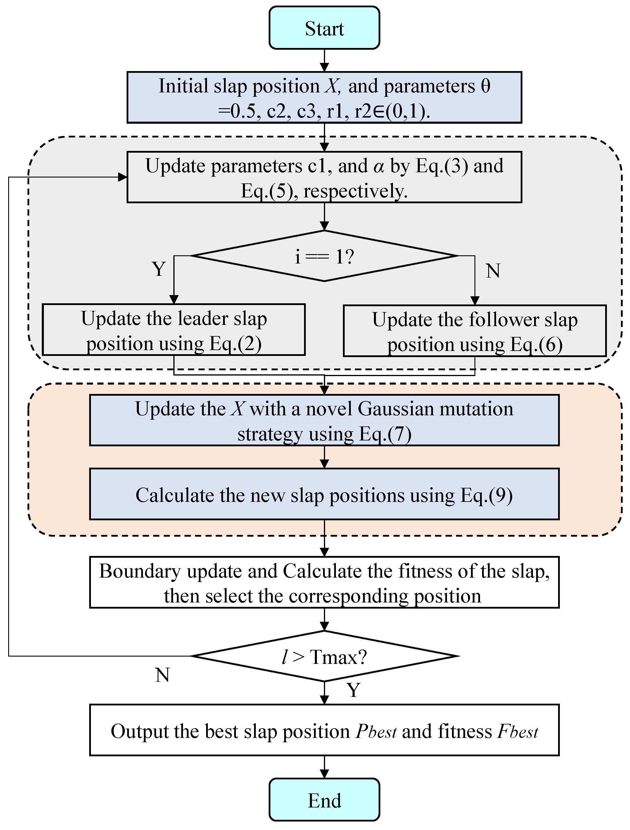
Figure 2 illustrates the flowchart of the EKSSA algorithm, detailing its optimization process. From Figure 2, it can be summarized in four stages. Stage 1 is the initialization of the slap position; Stage 2 includes parameter update, leader and follower position update of the proposed EKSSA; Stage 3 involves individual position update by the Gaussian mutation and mirror learning strategy. Stage 4 represents the best population of slaps corresponding to fitness during the optimization process. After the T m a x iterations of the designed method, the best solution and fitness value are generated.
To understand the main architecture of the method, the pseudo-code of the designed EKSSA is displayed in Algorithm 1. In particular, input, output, and the main code of the EKSSA are listed.
Algorithm 1: Pseudo-code of EKSSA.
Biomimetics 10 00638 i001

4. Results and Analysis

This section details the experimental setup, including the selected benchmark functions, algorithm hyperparameters, and the presentation of results from the CEC benchmarks and boxplot analyses.

4.1. Selected Benchmark Test Functions

A comprehensive evaluation of the proposed algorithm’s performance was conducted on 32 functions from the CEC benchmark suite [28,29,30,31], where F1 to F6 are unimodal (U), F7 to F10 are multimodal (M), and F11 to F18 are fixed-dimensional (M) functions, respectively. The dimension of F1 to F10 was wet at 30. Table 1 details the 18 functions. Table depicts eight functions (F19 to F26) from CEC2017 [30] and six functions (F27 to F32) from CEC2022 [31], respectively. For the experiment in this study, Matlab 2018a was the platform with a Windows 10 system, 16 GB memory, and Intel(R) (Santa Clara, CA, USA.) Core (TM) i5-10210U CPU @2.11 GHz.

4.2. Hyperparameter Settings

In our work, the performance and effectiveness of the designed EKSSA were assessed through a comprehensive suite of 32 numerical optimization benchmark functions. The comaprison algorithms are Randomized Particle Swarm Optimizer (RPSO) [32], Grey Wolf Optimizer (GWO) [5], Archimedes Optimization Algorithm (AOA) [33], Hybrid Particle Swarm Butterfly Algorithm (HPSBA) [34], Aquila Optimizer (AO) [7], Honey Badger Algorithm (HBA) [35], Salp Swarm Algorithm (SSA) [6], Sine–Cosine Quantum Salp Swarm Algorithm (SCQSSA) [36], and the proposed EKSSA. Notably, Table 2 presents the hyperparameter settings of the comparison approaches. For the optimization problem, the size of the population is set to 30 of all comparison approaches in this study, that is, N P = 30 . Each test function is executed independently 30 times, and the maximum number of iterations T m a x serves as the condition for optimization termination. T m a x is set to 1000 in this study.

4.3. Analysis of CEC Benchmark Function Results

From Table 3 containing the results of F1, F2, F3, F7, and F9, the proposed EKSSA can obtain the theoretical optimum, where Best, Worst, Mean, and Std are all the best. The smaller the STD value, the better the stability of the algorithm’s optimization of the comparison methods. For the fixed functions F16, F17, and F18, the EKSSA achieves the theoretical optimal value with the smallest Std value in the comparison methods. For the RPSO, its performance is better than that others on F13, F14, F15 under the best Std with theoretical optimum. In addition, the HPSBA can also obtain the same result as EKSSA in F1, F2, F3, F7, and F9; however, its performance should be improved on other benchmark functions. For F7 and F8, HBA, AO, HPSBA, SCQSSA and EKSSA have better results than others. For F9, HBA, AO, AOA, HPSBA, SCQSSA and EKSSA achieve the theoretical optimal value. From Table 3, the results show that EKSSA holds the top rank against the eight other methods over the suite of 18 test functions, and the overall ranking is EKSSA > HBA > AO > AOA > GWO > RPSO > SSA > HPSBA > SCQSSA. Also, Table 4 shows p-values of the comparison algorithms for F1 to F18 by the WSR test.
From Table 5, we report results on a collection of 14 test functions drawn from the CEC2017 and CEC2022 benchmarks with Mean, Std, Time, and p-value by the WSR test. For the Mean of F19, F20, F22, F23, F31, F32, the proposed EKSSA can obtain the best values comapred to other comparison algorithms. RPSO can obtain the best result from the Mean of F26, F27, and F29 compared to others. The performance of the EKSSA on complex numerical optimization problems is thus demonstrably effective. This is validated by the Friedman test results presented in Table 6, which ranks the algorithms based on their performance in 14 test functions of the CEC2017 and CEC2022 benchmark suites. The overall ranking is EKSSA > HBA > SSA > GWO > RPSO > AO > AOA > HPSBA > SCQSSA.
The empirical results in Table 3, Table 4, Table 5 and Table 6 indicate a modest increase in the optimization time of EKSSA compared to the basic SSA. This observed difference aligns with the conclusions drawn from the theoretical computational complexity analysis. For F1 with high dimension, the consumption time of the designed EKSSA is 1.6713E-01 s and the consumption time of the SSA is 1.6116E-01 s, which is approximately 0.006 s higher. For the F16 with fixed dimension, the consumption times of EKSSA and SSA are 2.7603E-01 s and 2.7019E-01 s, respectively, which is also approximately 0.006 s higher. Although the computational complexity is slightly higher, the performance of the proposed EKSSA is significantly improved compared to SSA from the results of the test functions.
Figure 3 and Figure 4 depict the convergence curves, which can be used to analyze the convergence speed and accuracy curve of comparison methods. From Figure 3, the EKSSA has better convergence than comparison methods with a fast speed on F1, F2, F3, and F8. From Figure 4, for F10, the convergence curve of EKSSA obtains the best value. For F5, F7, F10, and F12, the proposed EKSSA curves have multiple inflection points, indicating that it has a very good ability to escape from local optima. For other functions, the proposed EKSSA does not outperform all peers, indicating potential for further enhancement of its convergence properties in future work.

4.4. Boxplot Results Analysis

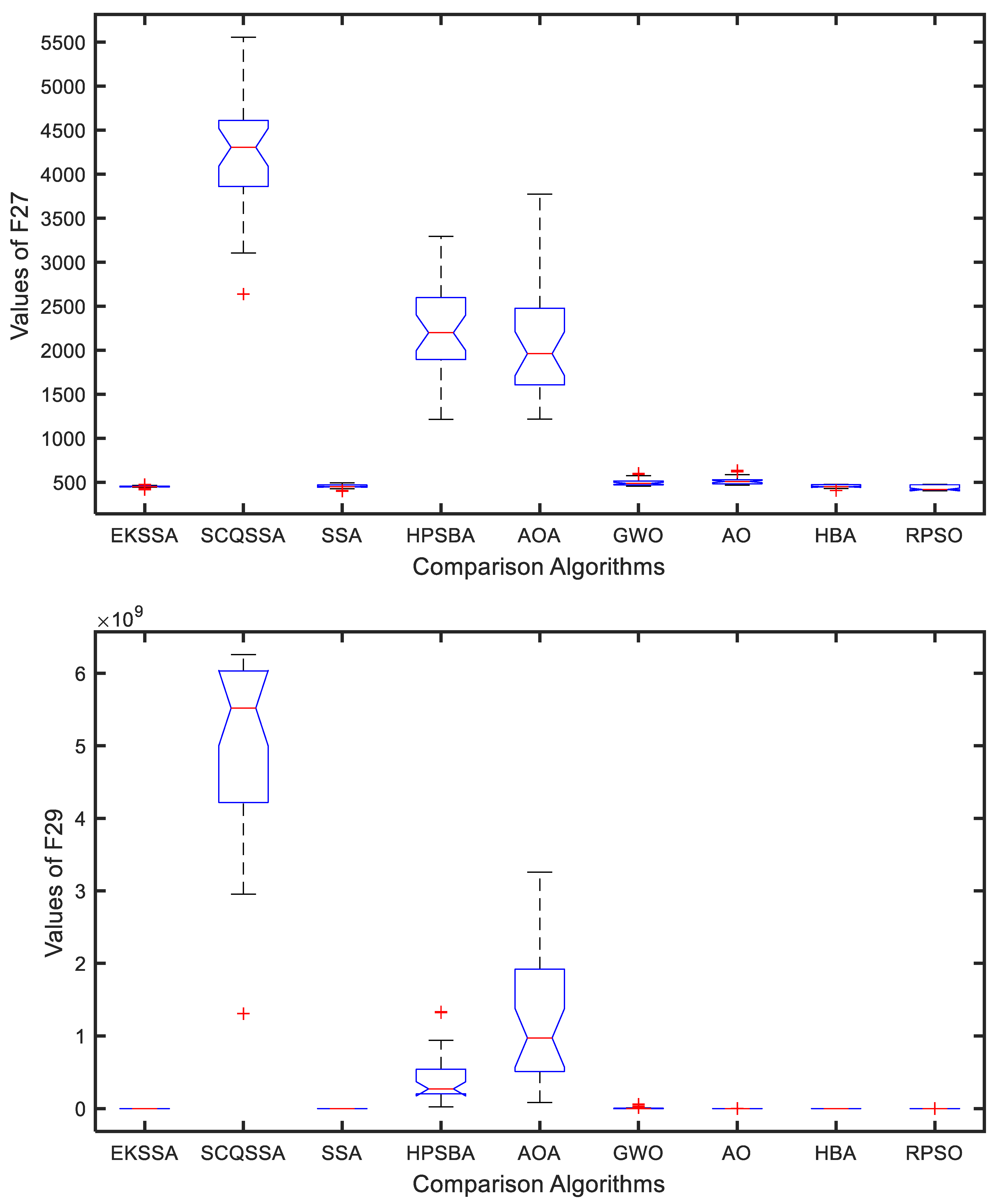
The boxplot can be used to explain the stability of the comparison approaches. Figure 5 and Figure 6 show the boxplot results of the nine comparison methods in F27, F29, F31, and F32. Notably, each algorithm was independently run 30 times for a test function. From Figure 5, EKSSA is better than others in F27. EKSSA, SSA, and HBA have a similar result to the boxplot of F29. In Figure 6, there are a few outliers in EKSSA from F31 and F32. The boxplot results demonstrate that the proposed EKSSA has better stability performance for the numerical optimization problem.

4.5. Ablation Results Analysis

To evaluate the contribution of each proposed strategy, ablation studies were conducted, and the results are summarized in Table 7. In this table, EKSSA1 denotes the algorithm that incorporates only adaptive adjustment strategies for parameters c 1 and α . EKSSA2 corresponds to the version that uses solely the novel position update strategy via Gaussian walk. EKSSA3 represents the configuration with only the dynamic mirror learning strategy. For comparison, the baseline SSA and fully integrated EKSSA are also included, which combines all three strategies. From Table 7, EKSSA1, EKSSA2, and EKSSA3 are all superior to basic SSA, indicating that the proposed improvement strategy is effective. The EKSSA that combines multiple strategies has the best performance, which indicates that the fusion of multiple strategies can effectively enhance the optimization ability of the algorithm and has a complementary effect.

5. Results of EKSSA-SVM for Seed Classification

High-quality seeds can help farmers achieve better profits and safe food. The classification of seeds through intelligent technology not only improves efficiency but also reduces the cost of manual screening. Thus, it is necessary for us to study the ML algorithm to identify seed varieties. The efficiency and accuracy of existing methods still hold potential for further improvement. Notably, there is also a gap for the seed classification task by the optimizing the hyperparameter of SVM using SIAs. In this research, two seed classification datasets were used to verify the performance of the proposed EKSSA. The SVM [37] served as the baseline model for seed classification, and the EKSSA was employed to optimize its hyperparameters, specifically the penalty coefficient c and the kernel parameter g.
Figure 7 presents the diagram of EKSSA-SVM for seed classification tasks using two Rice Varieties datasets from the open resources. There are two categories in the Rice Varieties Dataset 1, 1630 Cammeo and 2180 Osmancik [38]. Seven features ( f 1 , f 2 , , f M , M = 7 ) were sourced and consolidated with Area, Diameter, Major-axis length, Minor-axis length, Eccentricity, Convex-area, and Extent. In addition, Rice Varieties Dataset 2 has five categories: Arborio, Basmati, Ipsala, Jasmine, and Karacadag [39]; 10,000 samples were used for each category in this study. Sixteen features ( f 1 , f 2 , , f M , M = 16 ) were sourced and consolidated with Area, Perimeter, Major-Axis, Minor-Axis, Eccentricity, Eqdiasq, Solidity, Convex-Area, Extent, Aspect-Ratio, Roundness, Compactness, Shapefactor1, Shapefactor2, Shapefactor3, and Shapefactor4. The metric accuracy (Acc/%) is defined as:
A c c = T P + T N T P + T N + F P + F N × 100 % ,
where T P indicates the true positive number of the seed sample; T N denotes the true negative number of the seed sample. F P and F N are the false positive and negative number of the seed sample, respectively.
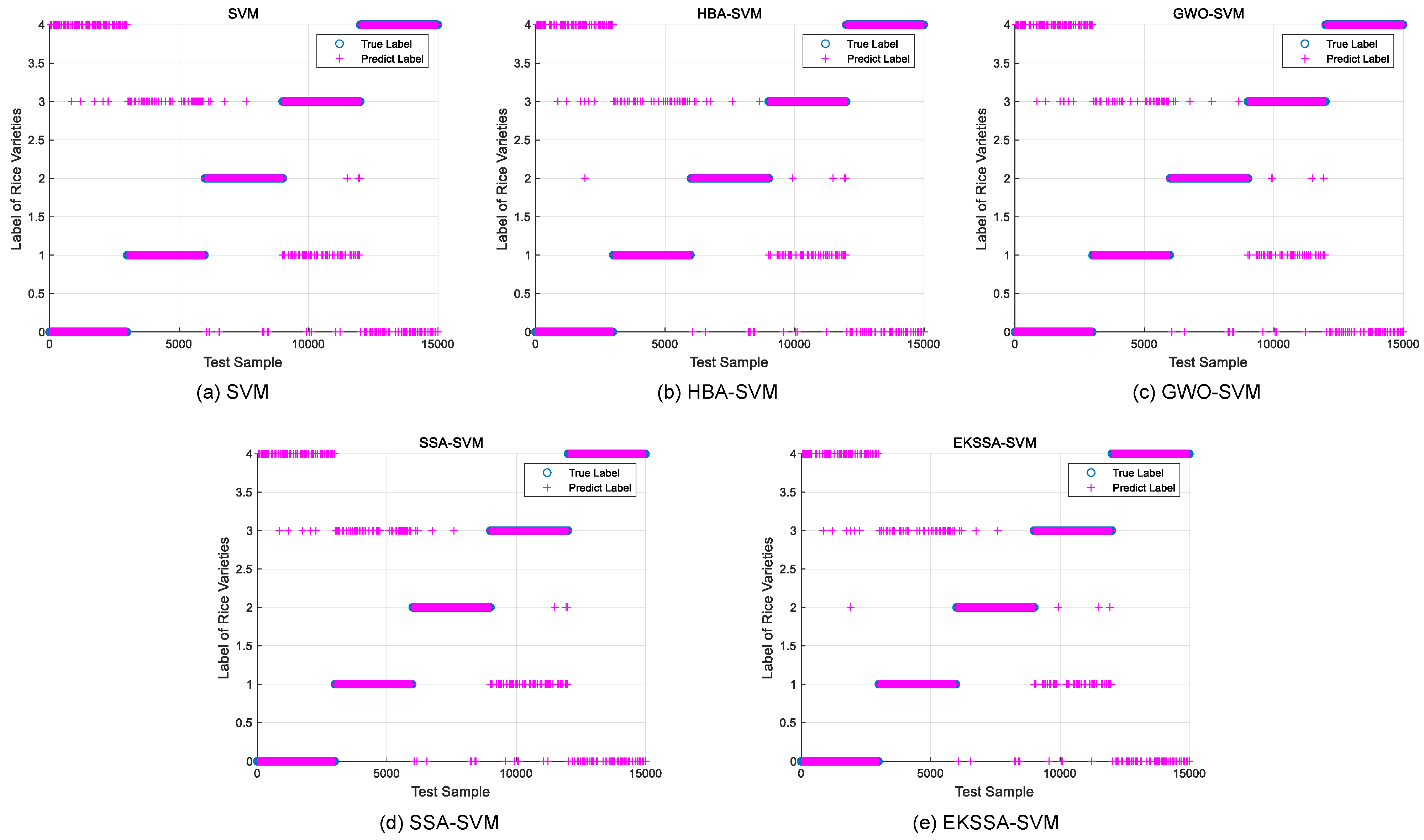
Notably, the features of the seed classification task are first normalized before being input into the classifier, which should be mapped between 0 and 1. The optimization of hyperparameters c and g significantly influences the predictive accuracy of the SVM model in the seed classification task. In these experiments, the dataset was partitioned into training and testing sets with a ratio of 7:3. The search intervals for c and g were set to [0.1, 5] and [0.1, 10], respectively. The population size was set to 10, and the iteration was set to 15. The comparison methods were selected from the top four ranking of the nine algorithms, which are EKSSA, HBA, SSA, and GWO. The results of Rice Varieties Dataset 1 and Dataset 2 are listed in Table 8 and Table 9, respectively. In addition, the true label and the predict label result is depicted in Figure 8 of the five methods.
For the Rice Varieties Dataset 1 in Table 8, test Acc (%) results of KNN, SVM, HBA-SSA, GWO-SVM, SSA-SVM, and EKSSA-SVM are 88.58, 90.5512 with c = 1 , g = 3 , 90.6387 with c = 4.16158 , g = 1.42268 , 90.8136 with c = 5 , g = 0.187119 , 90.7262 with c = 4.93214 , g = 0.241651 , and 90.8136 with c = 4.99847 , g = 0.187177 , respectively. Although the classification accuracy of EKSSA-SVM and GWO-SSA is the same, the c and g values for optimization are different.
For the Rice Varieties Dataset 2 in Table 9, the accuracy is 97.7867% by the basic SVM with c = 0.3 , g = 2 . SSA-SVM has 98.0667% Acc with c = 0.331123 , g = 1.95375 . GWO-SVM has 97.9600% Acc with c = 1.43546 , g = 2.67443 . HBA-SVM has 98.0667% Acc with c = 1.27977 , g = 8.6252 . The proposed EKSSA-SVM has 98.1133% Acc for the Rice Varieties classification task when c is set to 3.89383 and g is set to 6.03773. It is 0.3266, 0.0466, 0.1533, and 0.3466 percentage points higher than SVM, HBA-SVM, GWO-SVM, SSA-SVM, and EKSSA-SVM, respectively.
From Table 8 and Table 9, for different datasets, the values of parameter c and g are different by the proposed EKSSA-SVM. In addition, the true label and the predict label result of the five Rice Varieties dataset are depicted in Figure 9 of the SVM, HBA-SVM, GWO-SVM, SSA-SVM, and EKSSA-SVM. Except for Jasmine, there are obvious misclassification samples in the other types of Rice Varieties classification using Dataset 2. Thus, the predicted results of the EKSSA-SVM can be further modified by the quantum strategy.

6. Conclusions and Future Work

To address the deficiency that SSA is prone to fall into local optima, the EKSSA was designed and used to fill a gap for the seed classification task by optimizing the hyperparameter of SVM. Different adjustment strategies for the parameters c 1 and α are used to balance the exploration and exploitation of the slaps. Moreover, a novel position update strategy is inspired by the Gaussian walk theory, which improves the global search ability of the slap individual after the basic position update stage. Notably, a dynamic mirror learning strategy is designed to mirror the search range of the optimization problem with a local search capability. The performance of the EKSSA is verified by the thirty-two CEC benchmark functions, which is compared via eight advanced algorithms of RPSO, GWO, AOA, HPSBA, AO, HBA, SSA, and SCQSSA. In addition, a combined EKSSA-SVM classifier is proposed for the seed classification problem with a higher accuracy, in which EKSSA-SVM has 98.1133% Acc for the five Rice Varieties datasets when c is set to 3.89383 and g is set to 6.03773. In future work, chaotic population initialization and quantum strategies will be used to improve the performance of the EKSSA, which will be applied to solve the task of diagnosing plant leaf diseases [40].

Author Contributions

Conceptualization, Q.L. and Y.Z.; methodology, Q.L. and Y.Z.; software, Q.L.; validation, Q.L. and Y.Z.; formal analysis, Q.L. and Y.Z.; investigation, Q.L. and Y.Z.; resources, Y.Z.; data curation, Q.L. and Y.Z.; writing—original draft preparation, Q.L.; writing—review and editing, Q.L. and Y.Z.; visualization, Q.L. and Y.Z.; supervision, Y.Z.; project administration, Y.Z.; funding acquisition, Y.Z. All authors have read and agreed to the published version of the manuscript.

Funding

This study was funded by the Guangdong Basic and Applied Basic Research Foundation, grant numbers 2023A1515140021 and 2022A1515110757, and the Guangdong Academy of Agricultural Sciences Talent Introduction Project for 2022, grant number R2022YJ-YB3023.

Institutional Review Board Statement

Not applicable.

Informed Consent Statement

Not applicable.

Data Availability Statement

The Rice Varieties datasets can be found at https://www.muratkoklu.com/datasets/.

Conflicts of Interest

The authors declare no conflicts of interest.

References

  1. Kennedy, J.; Eberhart, R. Particle swarm optimization. In Proceedings of the ICNN’95-International Conference on Neural Networks, Perth, WA, Australia, 27 November–1 December 1995; Volume 4, pp. 1942–1948. [Google Scholar]
  2. Chakraborty, A.; Kar, A.K. Swarm intelligence: A review of algorithms. In Nature-Inspired Computing and Optimization; Springer: Cham, Switzerland, 2017; pp. 475–494. [Google Scholar]
  3. Zhang, M.; Wen, G. Duck swarm algorithm: Theory, numerical optimization, and applications. Clust. Comput. 2024, 27, 6441–6469. [Google Scholar] [CrossRef]
  4. Zhang, K.; Yuan, F.; Jiang, Y.; Mao, Z.; Zuo, Z.; Peng, Y. A Particle Swarm Optimization-Guided Ivy Algorithm for Global Optimization Problems. Biomimetics 2025, 10, 342. [Google Scholar] [CrossRef]
  5. Mirjalili, S.; Mirjalili, S.M.; Lewis, A. Grey wolf optimizer. Adv. Eng. Softw. 2014, 69, 46–61. [Google Scholar] [CrossRef]
  6. Mirjalili, S.; Gandomi, A.H.; Mirjalili, S.Z.; Saremi, S.; Faris, H.; Mirjalili, S.M. Salp Swarm Algorithm: A bio-inspired optimizer for engineering design problems. Adv. Eng. Softw. 2017, 114, 163–191. [Google Scholar] [CrossRef]
  7. Abualigah, L.; Yousri, D.; Abd Elaziz, M.; Ewees, A.A.; Al-Qaness, M.A.; Gandomi, A.H. Aquila optimizer: A novel meta-heuristic optimization algorithm. Comput. Ind. Eng. 2021, 157, 107250. [Google Scholar] [CrossRef]
  8. Abualigah, L.; Shehab, M.; Alshinwan, M.; Alabool, H. Salp swarm algorithm: A comprehensive survey. Neural Comput. Appl. 2020, 32, 11195–11215. [Google Scholar] [CrossRef]
  9. Wang, J.; Zhu, Z.; Zhang, F.; Liu, Y. An improved salp swarm algorithm for solving node coverage optimization problem in WSN. Peer-to-Peer Netw. Appl. 2024, 17, 1091–1102. [Google Scholar] [CrossRef]
  10. Zhou, H.; Shang, T.; Wang, Y.; Zuo, L. Salp Swarm Algorithm Optimized A* Algorithm and Improved B-Spline Interpolation in Path Planning. Appl. Sci. 2025, 15, 5583. [Google Scholar] [CrossRef]
  11. Khorashadizade, M.; Abbasi, E.; Fazeli, S.A.S. Improved salp swarm optimization algorithm based on a robust search strategy and a novel local search algorithm for feature selection problems. Chemom. Intell. Lab. Syst. 2025, 258, 105343. [Google Scholar] [CrossRef]
  12. Zhang, H.; Qin, X.; Gao, X.; Zhang, S.; Tian, Y.; Zhang, W. Improved salp swarm algorithm based on Newton interpolation and cosine opposition-based learning for feature selection. Math. Comput. Simul. 2024, 219, 544–558. [Google Scholar] [CrossRef]
  13. Wang, Y.; Cai, Z.; Guo, L.; Li, G.; Yu, Y.; Gao, S. A spherical evolution algorithm with two-stage search for global optimization and real-world problems. Inf. Sci. 2024, 665, 120424. [Google Scholar] [CrossRef]
  14. Saravanakumar, R.; TamilSelvi, T.; Pandey, D.; Pandey, B.K.; Mahajan, D.A.; Lelisho, M.E. Big data processing using hybrid Gaussian mixture model with salp swarm algorithm. J. Big Data 2024, 11, 167. [Google Scholar] [CrossRef]
  15. Wang, R.; Li, K.; Chen, P.; Tang, H. Multiple subpopulation Salp swarm algorithm with Symbiosis theory and Gaussian distribution for optimizing warm-up strategy of fuel cell power system. Appl. Energy 2025, 393, 126050. [Google Scholar] [CrossRef]
  16. Guo, L.; Xu, C.; Ai, X.; Han, X.; Xue, F. A Combined Forecasting Model Based on a Modified Pelican Optimization Algorithm for Ultra-Short-Term Wind Speed. Sustainability 2025, 17, 2081. [Google Scholar] [CrossRef]
  17. Li, F.; Dai, C.; Hussien, A.G.; Zheng, R. IPO: An Improved Parrot Optimizer for Global Optimization and Multilayer Perceptron Classification Problems. Biomimetics 2025, 10, 358. [Google Scholar] [CrossRef]
  18. Song, H.M.; Wang, J.S.; Hou, J.N.; Wang, Y.C.; Song, Y.W.; Qi, Y.L. Multi-strategy fusion pelican optimization algorithm and logic operation ensemble of transfer functions for high-dimensional feature selection problems. Int. J. Mach. Learn. Cybern. 2025, 16, 4433–4470. [Google Scholar] [CrossRef]
  19. Panneerselvam, R.; Balasubramaniam, S. Multi-Class Skin Cancer Classification using a hybrid dynamic salp swarm algorithm and weighted extreme learning machines with transfer learning. Acta Inform. Pragensia 2023, 12, 141–159. [Google Scholar] [CrossRef]
  20. Wang, Y.; Gao, S.; Yu, Y.; Cai, Z.; Wang, Z. A gravitational search algorithm with hierarchy and distributed framework. Knowl.-Based Syst. 2021, 218, 106877. [Google Scholar] [CrossRef]
  21. Yang, Z.; Jiang, Y.; Yeh, W.C. Self-learning salp swarm algorithm for global optimization and its application in multi-layer perceptron model training. Sci. Rep. 2024, 14, 27401. [Google Scholar] [CrossRef] [PubMed]
  22. Khan, I.R.; Sangari, M.S.; Shukla, P.K.; Aleryani, A.; Alqahtani, O.; Alasiry, A.; Alouane, M.T.H. An automatic-segmentation-and hyper-parameter-optimization-based artificial rabbits algorithm for leaf disease classification. Biomimetics 2023, 8, 438. [Google Scholar] [CrossRef]
  23. Koklu, M.; Ozkan, I.A. Multiclass classification of dry beans using computer vision and machine learning techniques. Comput. Electron. Agric. 2020, 174, 105507. [Google Scholar] [CrossRef]
  24. Islam, M.M.; Himel, G.M.S.; Moazzam, M.G.; Uddin, M.S. Artificial Intelligence-based Rice Variety Classification: A State-of-the-Art Review and Future Directions. Smart Agric. Technol. 2025, 10, 100788. [Google Scholar] [CrossRef]
  25. Saxena, P.; Priya, K.; Goel, S.; Aggarwal, P.K.; Sinha, A.; Jain, P. Rice varieties classification using machine learning algorithms. J. Pharm. Negat. Results 2022, 13, 3762–3772. [Google Scholar]
  26. Din, N.M.U.; Assad, A.; Dar, R.A.; Rasool, M.; Sabha, S.U.; Majeed, T.; Islam, Z.U.; Gulzar, W.; Yaseen, A. RiceNet: A deep convolutional neural network approach for classification of rice varieties. Expert Syst. Appl. 2024, 235, 121214. [Google Scholar] [CrossRef]
  27. Iqbal, M.J.; Aasem, M.; Ahmad, I.; Alassafi, M.O.; Bakhsh, S.T.; Noreen, N.; Alhomoud, A. On application of lightweight models for rice variety classification and their potential in edge computing. Foods 2023, 12, 3993. [Google Scholar] [CrossRef]
  28. Yao, X.; Liu, Y.; Lin, G. Evolutionary programming made faster. IEEE Trans. Evol. Comput. 1999, 3, 82–102. [Google Scholar] [CrossRef]
  29. Rashedi, E.; Nezamabadi-Pour, H.; Saryazdi, S. GSA: A gravitational search algorithm. Inf. Sci. 2009, 179, 2232–2248. [Google Scholar] [CrossRef]
  30. Wu, G.; Mallipeddi, R.; Suganthan, P.N. Problem Definitions and Evaluation Criteria for the CEC 2017 Competition on Constrained Real-Parameter Optimization; Technical Report; National University of Defense Technology: Changsha, China; Kyungpook National University: Daegu, Republic of Korea; Nanyang Technological University: Singapore, 2017. [Google Scholar]
  31. Bujok, P.; Kolenovsky, P. Eigen crossover in cooperative model of evolutionary algorithms applied to CEC 2022 single objective numerical optimisation. In Proceedings of the 2022 IEEE Congress on Evolutionary Computation (CEC), Padua, Italy, 18–23 July 2022; pp. 1–8. [Google Scholar]
  32. Liu, W.; Wang, Z.; Zeng, N.; Yuan, Y.; Alsaadi, F.E.; Liu, X. A novel randomised particle swarm optimizer. Int. J. Mach. Learn. Cybern. 2021, 12, 529–540. [Google Scholar] [CrossRef]
  33. Hashim, F.A.; Hussain, K.; Houssein, E.H.; Mabrouk, M.S.; Al-Atabany, W. Archimedes optimization algorithm: A new metaheuristic algorithm for solving optimization problems. Appl. Intell. 2021, 51, 1531–1551. [Google Scholar] [CrossRef]
  34. Zhang, M.; Wang, D.; Yang, M.; Tan, W.; Yang, J. HPSBA: A modified hybrid framework with convergence analysis for solving wireless sensor network coverage optimization problem. Axioms 2022, 11, 675. [Google Scholar] [CrossRef]
  35. Hashim, F.A.; Houssein, E.H.; Hussain, K.; Mabrouk, M.S.; Al-Atabany, W. Honey Badger Algorithm: New metaheuristic algorithm for solving optimization problems. Math. Comput. Simul. 2022, 192, 84–110. [Google Scholar] [CrossRef]
  36. Jia, F.; Luo, S.; Yin, G.; Ye, Y. A novel variant of the salp swarm algorithm for engineering optimization. J. Artif. Intell. Soft Comput. Res. 2023, 13, 131–149. [Google Scholar] [CrossRef]
  37. Chang, C.C.; Lin, C.J. LIBSVM: A library for support vector machines. ACM Trans. Intell. Syst. Technol. 2011, 2, 27. [Google Scholar] [CrossRef]
  38. Cinar, I.; Koklu, M. Classification of rice varieties using artificial intelligence methods. Int. J. Intell. Syst. Appl. Eng. 2019, 7, 188–194. [Google Scholar] [CrossRef]
  39. Koklu, M.; Cinar, I.; Taspinar, Y.S. Classification of rice varieties with deep learning methods. Comput. Electron. Agric. 2021, 187, 106285. [Google Scholar] [CrossRef]
  40. Wang, A.; Song, Z.; Xie, Y.; Hu, J.; Zhang, L.; Zhu, Q. Detection of Rice Leaf SPAD and Blast Disease Using Integrated Aerial and Ground Multiscale Canopy Reflectance Spectroscopy. Agriculture 2024, 14, 1471. [Google Scholar] [CrossRef]
Figure 1. The curve of the parameter α .
Biomimetics 10 00638 g001
Figure 2. The flowchart of the designed EKSSA.
Biomimetics 10 00638 g002
Figure 3. Convergence curves of the comparison algorithms on F1 to F3, F5, F7, and F8.
Biomimetics 10 00638 g003
Figure 4. Convergence curves of the comparison algorithms on F9 to F12, F14, and F17.
Biomimetics 10 00638 g004
Figure 5. Boxplot for F27 and F29 of the comparison methods.
Biomimetics 10 00638 g005
Figure 6. Boxplot for F31 and F32 of the comparison methods.
Biomimetics 10 00638 g006
Figure 7. The diagram of the EKSSA-SVM for seed classification.
Biomimetics 10 00638 g007
Figure 8. Predict results of the comparison approaches for Rice Varieties Dataset 1.
Biomimetics 10 00638 g008
Figure 9. Predict results of the comparison approaches for Rice Varieties Dataset 2.
Biomimetics 10 00638 g009
Table 1. Eighteen test functions for the performance evaluation.
FormulaRangeDim f min Category
F 1 = i = 1 D i m x i 2 [−100, 100]300U
F 2 = i = 1 D i m j = 1 i x j 2 [−100, 100]300U
F 3 = max x i , 1 i D i m [−100, 100]300U
F 4 = i = 1 D i m 100 x i + 1 x i 2 2 + x i 1 2 [−30,30]300U
F 5 = i = 1 D i m x i + 0.5 2 [−100, 100]300U
F 6 = i = 1 D i m i x i 4 + r a n d ( 0 ,   1 ) [−1.28, 1.28]300U
F 7 = i = 1 D i m x i 2 10 cos ( 2 π x i ) + 10 [−5.12, 5.12]300M
F 8 = 20 exp 0.2 1 D i m i = 1 D i m x i 2 exp 1 D i m i = 1 D i m cos ( 2 π x i ) + 20 + e [−32, 32]300M
F 9 = 1 4000 i = 1 D i m x i 2 i = 1 D i m cos x i i + 1 [−600, 600]300M
F 10 = π D i m i = 1 D i m 1 ( y i 1 ) 2 [ 1 + 10 sin 2 ( π y i + 1 ) ] + ( y D i m 1 ) 2 + 10 sin 2 ( π y 1 ) + i = 1 D i m u ( x i , 10 , 100 , 4 ) , y i = 1 + x i + 1 4 , u y i , a , k , m = k ( x i a ) m , x i > a , 0 , a x i a , k ( x i a ) m , x i < a [−50, 50]300M
F 11 = 1 500 + j = 1 25 1 j + i = 1 2 x i a i j 6 1 [−65, 65]21Fixed
F 12 = i = 1 11 a i x 1 ( b i 2 + b i x 2 ) b i 2 + b i x 3 + x 4 2 [−5, 5]40.00030Fixed
F 13 = 4 x 1 2 2.1 x 1 4 + 1 3 x 1 6 + x 1 x 2 4 x 2 2 + 4 x 2 4 [−5, 5]2−1.0316Fixed
F 14 = 1 + x 1 + x 2 + 1 2 19 14 x 1 + 3 x 1 2 14 x 2 + 6 x 1 x 2 + 3 x 2 2 × 30 + 2 x 1 3 x 2 2 × 18 32 x 1 + 12 x 1 2 + 48 x 2 36 x 1 x 2 + 27 x 2 2 [−2, 2]23Fixed
F 15 = i = 1 4 c i exp j = 1 3 a i j x j p i j 2 [1, 3]3−3.86Fixed
F 16 = i = 1 5 ( X a i ) ( X a i ) + c i 1 [0, 10]4−10.1532Fixed
F 17 = i = 1 7 ( X a i ) ( X a i ) + c i 1 [0, 10]4−10.4028Fixed
F 18 = i = 1 10 ( X a i ) ( X a i ) + c i 1 [0, 10]4−10.5363Fixed
Table 2. Comparison of algorithm hyperparameter settings.
AlgorithmsHyperparameter
RPSO [32] c p , m a x = c g , m a x = 2.5 , c p , m i n = c g , m i n = 0.5 , ω m i n = 0.2 , ω m a x = 0.9 , V m a x = 1.5
GWO [5] a f i r s t = 2 , a f i n a l = 0
AOA [33] C 1 = 2 , C 2 = 6 , C 3 = 1 , C 4 = 2 , μ = 0.9 , L = 0.1
HPSBA [34] a = 0.1 , c ( 0 ) = 0.35 , S P = 0.6 , μ = 4 , ω u = 0.9 , ω l = 0.2 , C 1 = C 2 = 2 , V m a x = 1
AO [7] α = 0.1 , δ = 0.1 , u = 0.0265 , r 0 = 10
HBA [35] C = 2 , β = 6 , r 1 t o r 4 ( 0 , 1 )
SSA [6] c 2 , c 3 ( 0 , 1 )
SCQSSA [36] a = 2 , r = 0.5 , c 2 , c 3 , c 4 ( 0 , 1 )
EKSSA θ = 0.5 , c 2 , c 3 ( 0 , 1 ) , r 1 , r 2 ( 0 , 1 )
Table 3. Comparative evaluation of nine algorithms using 18 benchmark functions.
Fun.ItemRPSOHBAAOGWOAOAHPSBASSASCQSSAEKSSA
F1Best1.0871E-055.0979E-2862.1672E-3024.6005E-616.8467E-2700.0000E+007.9382E-093.4286E-1430.0000E+00
Worst4.1424E-033.1094E-2757.0015E-1984.3320E-582.8345E-1700.0000E+002.1899E-085.2806E-1310.0000E+00
Mean3.4513E-041.1435E-2763.1090E-1996.3414E-591.0401E-1710.0000E+001.2965E-082.1250E-1320.0000E+00
Std7.4244E-040.0000E+000.0000E+001.0112E-580.0000E+000.0000E+003.4796E-099.7067E-1320.0000E+00
Median1.6531E-041.8544E-2804.1845E-2872.5257E-593.2191E-2020.0000E+001.2252E-082.3128E-1360.0000E+00
Time/s7.6739E-022.3857E-012.5940E-011.8745E-011.6116E-012.0342E-011.6667E-018.3104E-011.6713E-01
F2Best1.6665E+002.4658E-2192.0469E-3002.2524E-209.4293E-2150.0000E+005.4015E+011.3441E-1430.0000E+00
Worst2.5062E+016.5791E-2024.6860E-1933.3923E-143.1095E-1300.0000E+001.2339E+031.8284E-1250.0000E+00
Mean8.7402E+002.8131E-2031.5620E-1944.2494E-151.0365E-1310.0000E+002.8990E+026.5991E-1270.0000E+00
Std5.1008E+000.0000E+000.0000E+008.8180E-155.6771E-1310.0000E+002.1942E+023.3383E-1260.0000E+00
Median7.5736E+001.4701E-2093.7262E-2791.4928E-163.9345E-1730.0000E+002.4519E+022.0619E-1340.0000E+00
Time/s/s3.2722E-014.9403E-017.6181E-014.2974E-014.1021E-016.8059E-014.1281E-011.1040E+004.1676E-01
F3Best1.3808E-011.3574E-1241.3873E-1513.9650E-166.2441E-1170.0000E+001.7994E+001.0777E-730.0000E+00
Worst4.4836E-018.7589E-1181.2381E-1018.8627E-143.2709E-790.0000E+001.6331E+016.5961E-650.0000E+00
Mean2.6266E-016.9002E-1194.1270E-1031.3036E-141.0904E-800.0000E+007.1955E+002.4068E-660.0000E+00
Std7.8817E-021.8666E-1182.2604E-1021.7775E-145.9717E-800.0000E+003.4866E+001.2017E-650.0000E+00
Median2.4784E-011.8064E-1201.7965E-1458.2225E-153.1810E-920.0000E+007.1382E+001.1317E-680.0000E+00
Time/s7.8774E-022.3851E-012.6371E-011.8261E-011.6240E-011.8497E-011.5898E-018.4002E-011.6551E-01
F4Best2.2844E+012.0236E+019.5558E-062.5265E+012.8682E+012.8893E+012.5476E+012.8298E+012.8302E+01
Worst9.3042E+012.2669E+013.2068E-032.8550E+012.8953E+012.8990E+011.6919E+032.8966E+012.8553E+01
Mean3.9698E+012.1840E+017.9130E-042.6775E+012.8868E+012.8945E+011.9731E+022.8842E+012.8492E+01
Std2.4343E+015.6739E-018.5900E-047.9266E-017.5559E-022.4464E-023.4706E+021.3987E-016.2818E-02
Median2.8633E+012.1824E+014.0502E-042.7038E+012.8910E+012.8951E+014.8841E+012.8860E+012.8507E+01
Time/s1.0746E-012.7113E-013.2625E-012.1368E-011.8402E-012.4121E-011.9279E-018.6755E-011.9446E-01
F5Best3.0734E-064.5395E-092.3206E-071.0059E-054.7257E+005.6910E+006.0874E-097.5000E+009.3936E-09
Worst6.4403E-035.4570E-071.1377E-041.5042E+006.1407E+007.2786E+002.0411E-087.5000E+002.2061E-08
Mean4.7903E-048.3845E-082.0746E-056.2593E-015.6421E+007.0171E+001.2264E-087.5000E+001.3787E-08
Std1.2043E-031.3975E-073.2782E-053.5178E-013.3251E-012.9880E-012.9866E-090.0000E+002.7012E-09
Median1.3118E-043.0803E-085.5117E-065.0430E-015.7044E+007.0965E+001.2092E-087.5000E+001.3364E-08
Time/s7.5309E-022.3935E-012.5858E-011.8246E-011.5366E-011.7462E-011.5705E-018.3671E-011.6495E-01
F6Best3.5978E-023.2280E-053.3284E-061.4142E-044.5308E-052.0666E-072.5736E-029.6596E-078.7290E-06
Worst1.9572E-016.7496E-044.0907E-042.6931E-037.8691E-041.9422E-041.6190E-011.1648E-048.5701E-04
Mean8.8336E-022.3684E-048.6043E-058.5170E-042.8454E-043.4069E-059.1888E-023.8346E-052.0673E-04
Std3.8992E-021.7220E-049.0615E-055.8252E-042.1355E-044.6980E-052.9178E-022.9220E-051.8859E-04
Median8.3680E-021.8803E-045.1356E-056.8982E-041.9379E-041.6572E-059.2231E-023.1997E-051.6195E-04
Time/s1.9892E-013.6235E-015.0788E-013.0756E-012.8211E-014.2448E-012.8335E-019.5296E-012.8817E-01
F7Best2.5183E+010.0000E+000.0000E+000.0000E+000.0000E+000.0000E+002.6864E+010.0000E+000.0000E+00
Worst8.8570E+010.0000E+000.0000E+001.1369E-131.3016E+020.0000E+008.7556E+010.0000E+000.0000E+00
Mean4.6916E+010.0000E+000.0000E+001.3263E-144.3388E+000.0000E+005.7276E+010.0000E+000.0000E+00
Std1.3985E+010.0000E+000.0000E+002.8649E-142.3764E+010.0000E+001.7429E+010.0000E+000.0000E+00
Median4.5899E+010.0000E+000.0000E+000.0000E+000.0000E+000.0000E+005.8702E+010.0000E+000.0000E+00
Time/s9.9330E-022.4508E-012.8035E-011.9433E-011.6327E-011.9794E-011.7681E-018.3219E-011.8004E-01
F8Best1.6858E-038.8818E-168.8818E-167.9936E-158.8818E-168.8818E-162.5278E-058.8818E-168.8818E-16
Worst2.7782E-028.8818E-168.8818E-162.2204E-141.9967E+018.8818E-164.3829E+008.8818E-168.8818E-16
Mean9.5237E-038.8818E-168.8818E-161.5810E-141.2645E+018.8818E-161.8865E+008.8818E-168.8818E-16
Std6.4119E-030.0000E+000.0000E+003.2854E-159.7857E+000.0000E+001.0589E+000.0000E+000.0000E+00
Median8.0054E-038.8818E-168.8818E-161.5099E-141.9963E+018.8818E-162.1201E+008.8818E-168.8818E-16
Time/s9.9029E-022.5644E-012.9403E-011.9403E-011.8036E-012.1217E-011.8586E-018.5280E-011.9181E-01
F9Best5.7578E+000.0000E+000.0000E+000.0000E+000.0000E+000.0000E+003.1355E-080.0000E+000.0000E+00
Worst2.0247E+010.0000E+000.0000E+001.5965E-020.0000E+000.0000E+003.6916E-020.0000E+000.0000E+00
Mean1.2628E+010.0000E+000.0000E+008.4343E-040.0000E+000.0000E+009.9315E-030.0000E+000.0000E+00
Std4.2599E+000.0000E+000.0000E+003.3256E-030.0000E+000.0000E+009.6595E-030.0000E+000.0000E+00
Median1.2327E+010.0000E+000.0000E+000.0000E+000.0000E+000.0000E+009.8574E-030.0000E+000.0000E+00
Time/s1.2764E-012.7863E-013.3153E-012.2109E-011.8755E-012.4667E-012.0475E-018.6659E-012.1296E-01
F10Best5.4730E-072.6154E-101.5131E-081.3102E-023.1349E-017.2340E-012.9569E-011.6690E+005.2730E-11
Worst3.2205E+002.0290E-074.4939E-067.9633E-021.2967E+001.4506E+001.2787E+011.6690E+002.8605E-10
Mean6.4483E-012.0073E-086.9802E-073.5659E-028.8141E-011.1766E+004.3187E+001.6690E+001.3092E-10
Std7.7438E-014.7279E-089.9589E-071.5691E-022.4309E-011.4058E-012.9416E+001.1292E-155.5764E-11
Median4.1377E-013.8722E-093.0096E-073.4152E-028.9735E-011.1993E+004.0085E+001.6690E+001.1875E-10
Time/s4.2600E-016.0956E-019.5677E-015.3195E-015.0738E-018.8628E-015.1287E-011.1734E+005.2058E-01
F11Best9.9800E-019.9800E-019.9800E-019.9800E-019.9800E-011.9921E+009.9800E-013.9933E+009.9800E-01
Worst5.9288E+001.0763E+011.0763E+011.2671E+012.3278E+001.2671E+019.9800E-011.2671E+019.9800E-01
Mean1.8884E+001.8142E+002.1121E+004.2584E+001.1788E+001.1179E+019.9800E-011.0006E+019.9800E-01
Std1.4963E+002.5154E+002.4850E+004.3765E+003.9455E-013.1144E+002.5250E-162.9956E+003.7224E-16
Median9.9800E-019.9800E-019.9800E-012.9821E+009.9833E-011.2671E+019.9800E-011.1761E+019.9800E-01
Time/s6.8657E-018.2461E-011.5141E+007.1329E-017.2139E-011.4306E+007.6984E-018.0659E-017.7094E-01
F12Best3.0749E-043.0749E-043.2106E-043.0749E-043.1219E-043.1100E-033.0913E-047.2945E-044.4368E-04
Worst1.2899E-032.2553E-026.3536E-042.0363E-021.8970E-031.0530E-012.0366E-021.1743E-022.0363E-02
Mean5.1152E-043.9645E-034.5475E-045.0545E-036.6017E-046.7976E-022.7495E-033.1134E-032.0420E-03
Std3.1782E-048.0783E-038.6007E-058.5930E-033.2773E-043.0996E-025.9782E-032.6091E-034.9868E-03
Median3.3371E-043.0749E-044.3970E-043.0756E-045.5994E-048.1765E-027.4679E-042.4190E-036.7069E-04
Time/s3.7391E-021.7746E-011.9967E-017.3134E-028.3582E-021.3615E-011.1911E-012.0999E-011.2642E-01
F13Best−1.0316E+00−1.0316E+00−1.0316E+00−1.0316E+00−1.0316E+00−1.0288E+00−1.0316E+00−1.0285E+00−1.0316E+00
Worst−1.0316E+00−1.0316E+00−1.0305E+00−1.0316E+00−1.0298E+00−1.9676E-01−1.0316E+00−9.1327E-01l−1.0316E+00
Mean−1.0316E+00−1.0316E+00−1.0315E+00−1.0316E+00−1.0316E+00−8.6481E-01−1.0316E+00−9.9579E-01−1.0316E+00
Std6.6486E-166.5843E-162.1811E-049.3022E-093.3084E-042.2396E-017.6308E-152.1560E-023.4146E-14
Median−1.0316E+00−1.0316E+00−1.0315E+00−1.0316E+00−1.0316E+00−9.6487E-01−1.0316E+00−9.9841E-01−1.0316E+00
Time/s3.3963E-021.6545E-011.8914E-016.2955E-027.7229E-021.3278E-011.1134E-011.6107E-011.2497E-01
F14Best3.0000E+003.0000E+003.0001E+003.0000E+003.0000E+003.0000E+003.0000E+003.5372E+003.0000E+00
Worst3.0000E+003.0000E+003.0538E+008.4000E+017.0164E+003.4475E+013.0000E+009.2105E+013.0000E+00
Mean3.0000E+003.0000E+003.0119E+005.7000E+003.4668E+009.4564E+003.0000E+002.3362E+013.0000E+00
Std1.6637E-151.8124E-151.2577E-021.4789E+011.1102E+001.1919E+011.0956E-131.8877E+012.2873E-13
Median3.0000E+003.0000E+003.0058E+003.0000E+003.0002E+003.0010E+003.0000E+001.9620E+013.0000E+00
Time/s2.2985E-021.5308E-011.6649E-015.1694E-026.6687E-021.0908E-011.0242E-011.4711E-011.0659E-01
F15Best−3.8628E+00−3.0048E-01−3.0048E-01l−3.0048E-01−3.5146E+00−3.0048E-01−3.0048E-01l−3.0048E-01−3.0048E-01
Worst−3.8628E+00−3.0048E-01−3.0048E-01−3.0048E-01−7.9410E-01−3.0048E-01−3.0048E-01−3.0048E-01−3.0048E-01
Mean−3.8628E+00−3.0048E-01−3.0048E-01−3.0048E-01−2.6868E+00−3.0048E-01−3.0048E-01−3.0048E-01−3.0048E-01
Std2.6962E-152.2584E-162.2584E-162.2584E-167.2118E-012.2584E-162.2584E-162.2584E-162.2584E-16
Median−3.8628E+00−3.0048E-01−3.0048E-01−3.0048E-01−2.7402E+00−3.0048E-01−3.0048E-01−3.0048E-01−3.0048E-01
Time/s4.3984E-021.7840E-012.1879E-018.0353E-027.4867E-021.6007E-011.2369E-011.9545E-011.3739E-01
F16Best−1.0153E+01−1.0153E+01−1.0153E+01−1.0153E+01−1.0107E+01−4.7195E+00−1.0153E+01−7.8746E+00−1.0153E+01
Worst−2.6305E+00−2.6305E+00−1.0130E+01−5.0552E+00−2.7971E+00−3.0807E-01−2.6305E+00−1.1705E+00−1.0153E+01
Mean−6.2309E+00−9.4009E+00−1.0149E+01−9.1408E+00−7.0359E+00−1.2026E+00−7.4807E+00−2.6948E+00−1.0153E+01
Std3.5747E+002.2954E+005.9610E-032.0586E+002.5106E+001.3025E+003.4095E+001.9091E+003.4774E-11
Median−5.0552E+00−1.0153E+01−1.0152E+01−1.0153E+01−7.4458E+00−7.3822E-01−1.0153E+01−1.7999E+00−1.0153E+01
Time/s1.8072E-013.2544E-014.9822E-012.1532E-012.2460E-014.3290E-012.7019E-013.5169E-012.7603E-01
F17Best−1.0403E+01−1.0403E+01−1.0403E+01−1.0403E+01−1.0399E+01−4.8638E+00−1.0403E+01−5.2867E+00−1.0403E+01
Worst−2.7519E+00−2.7659E+00−1.0374E+01−1.0402E+01−3.4804E+00−3.6735E-01−2.7519E+00−1.0021E+00−1.0403E+01
Mean−7.2807E+00−8.7488E+00−1.0399E+01−1.0402E+01−7.0277E+00−1.9336E+00−9.1109E+00−2.3042E+00−1.0403E+01
Std3.6770E+003.0586E+006.6812E-033.0980E-042.6085E+001.3987E+002.6831E+009.7513E-013.7219E-11
Median−1.0403E+01−1.0403E+01−1.0401E+01−1.0402E+01−7.5839E+00−1.4065E+00−1.0403E+01−2.0145E+00−1.0403E+01
Time/s2.4129E-013.9195E-016.2608E-012.8672E-012.9807E-015.7434E-013.3569E-014.4305E-013.4653E-01
F18Best−1.0536E+01−1.0536E+01−1.0536E+01−1.0536E+01−1.0533E+01−4.5544E+00−1.0536E+01−8.1276E+00−1.0536E+01
Worst−2.4217E+00−1.8595E+00−1.0497E+01−1.0535E+01−2.5691E+00−4.8413E-01−2.4273E+00−9.9274E-01−1.0536E+01
Mean−6.9934E+00−8.9549E+00−1.0532E+01−1.0536E+01−7.6711E+00−2.2185E+00−1.0086E+01−3.0340E+00−1.0536E+01
Std3.7086E+003.2289E+008.8857E-032.5735E-042.7035E+001.2678E+001.7510E+001.8349E+003.7452E-11
Median−7.8560E+00−1.0536E+01−1.0535E+01−1.0536E+01−8.3417E+00−1.8073E+00−1.0536E+01−2.0964E+00−1.0536E+01
Time/s3.2085E-014.7751E-017.7526E-013.5927E-013.6384E-017.0915E-014.0120E-014.9163E-014.1779E-01
Friedman Test5.184.274.505.104.945.735.696.383.21
Rank623548791
Table 4. WSR test p-values of eight algorithms with designed EKSSA.
FunctionsRPSOHBAAOGWOAOAHPSBASSASCQSSA
F11.73E-061.73E-061.73E-061.73E-061.73E-061.00E+001.73E-061.73E-06
F21.73E-061.73E-061.73E-061.73E-061.73E-061.00E+001.73E-061.73E-06
F31.73E-061.73E-061.73E-061.73E-061.73E-061.00E+001.73E-061.73E-06
F41.73E-061.73E-061.73E-062.13E-061.73E-061.73E-066.84E-031.92E-06
F51.73E-063.32E-041.73E-061.73E-061.73E-061.73E-068.59E-021.73E-06
F61.73E-065.86E-015.71E-041.73E-061.41E-011.97E-051.73E-061.24E-05
F71.73E-061.00E+001.00E+003.13E-021.00E+001.00E+001.73E-061.00E+00
F81.73E-061.00E+001.00E+007.99E-072.69E-051.00E+001.73E-061.00E+00
F91.73E-061.00E+001.00E+005.00E-011.00E+001.00E+001.73E-061.00E+00
F101.73E-061.73E-061.73E-061.73E-061.73E-061.73E-061.73E-061.73E-06
F113.68E-036.52E-021.73E-061.73E-061.73E-061.73E-061.25E-011.73E-06
F129.84E-032.13E-011.24E-055.58E-014.07E-021.73E-064.41E-015.29E-04
F131.63E-061.63E-061.73E-061.73E-061.73E-061.73E-067.00E-051.73E-06
F141.73E-061.73E-061.73E-061.73E-061.73E-061.73E-062.32E-041.73E-06
F154.32E-081.00E+001.00E+001.00E+001.73E-061.00E+001.00E+001.00E+00
F163.61E-032.77E-031.73E-061.73E-061.73E-061.73E-061.02E-011.73E-06
F171.02E-013.71E-011.73E-061.73E-061.73E-061.73E-067.97E-011.73E-06
F182.07E-021.65E-011.73E-061.73E-061.73E-061.73E-065.32E-031.73E-06
Table 5. Results of the nine comparison methods on the CEC2017 and CEC2022 benchmark functions with WSR test.
FunctionsItemEKSSASCQSSASSAHPSBAAOAGWOAOHBARPSO
F19Mean5.00E+021.73E+045.10E+021.47E+041.19E+046.28E+026.62E+025.05E+024.74E+02
Std1.32E+012.49E+032.70E+013.92E+032.49E+031.13E+027.71E+012.79E+012.53E+01
Time2.59E-019.31E-012.53E-013.84E-012.62E-013.00E-014.77E-012.81E-011.73E-01
p-value/1.73E-061.16E-011.73E-061.73E-061.73E-061.73E-062.71E-011.15E-04
F20Mean6.21E+021.00E+036.70E+029.08E+028.70E+026.27E+027.10E+026.27E+027.30E+02
Std3.77E+011.95E+013.95E+013.54E+012.52E+014.32E+013.45E+013.35E+013.38E+01
Time3.05E-019.85E-012.86E-014.44E-012.83E-013.15E-015.24E-013.08E-012.00E-01
p-value/1.73E-066.89E-051.73E-061.73E-066.73E-011.92E-063.39E-012.35E-06
F21Mean6.35E+027.10E+026.50E+026.88E+026.79E+026.12E+026.48E+026.15E+026.54E+02
Std1.12E+016.30E+001.44E+017.50E+006.41E+004.94E+007.38E+006.61E+008.91E+00
Time4.01E-011.10E+004.12E-016.89E-014.05E-014.53E-017.57E-014.20E-013.19E-01
p-value/1.73E-061.15E-041.73E-061.73E-062.13E-061.74E-041.92E-063.11E-05
F22Mean2.77E+034.36E+032.78E+033.61E+033.53E+032.78E+032.96E+032.81E+033.46E+03
Std3.27E+012.55E+023.06E+011.46E+021.47E+024.66E+017.72E+014.59E+011.46E+02
Time5.48E-011.22E+005.39E-019.40E-015.30E-015.59E-011.03E+005.54E-014.46E-01
p-value/1.73E-066.14E-011.73E-061.73E-069.43E-011.73E-061.29E-031.73E-06
F23Mean2.93E+034.61E+032.95E+033.85E+033.87E+032.96E+033.09E+033.03E+033.43E+03
Std3.53E+012.43E+023.34E+012.17E+021.82E+025.43E+015.17E+011.51E+021.21E+02
Time5.83E-011.27E+005.81E-011.02E+005.72E-016.01E-011.11E+005.94E-014.90E-01
p-value/1.73E-061.99E-011.73E-061.73E-061.04E-021.73E-062.41E-041.73E-06
F24Mean2.91E+036.06E+032.92E+035.02E+034.74E+033.00E+032.99E+032.90E+032.91E+03
Std2.96E+015.29E+022.45E+014.75E+023.92E+023.45E+012.68E+011.40E+012.13E+01
Time5.28E-011.20E+005.20E-019.09E-015.13E-015.43E-019.97E-015.42E-014.32E-01
p-value/1.73E-068.97E-021.73E-061.73E-061.73E-061.73E-061.75E-029.43E-01
F25Mean3.27E+035.48E+033.26E+034.39E+033.59E+033.26E+033.39E+033.36E+033.92E+03
Std3.62E+014.81E+022.73E+014.56E+025.57E+022.58E+017.17E+011.64E+023.15E+02
Time6.99E-011.37E+006.94E-011.25E+006.83E-017.16E-011.35E+007.07E-016.04E-01
p-value/1.73E-061.02E-011.73E-062.06E-015.17E-012.60E-062.26E-031.73E-06
F26Mean3.39E+037.70E+033.26E+037.01E+035.97E+033.45E+033.42E+033.24E+033.22E+03
Std6.00E+025.80E+022.07E+016.45E+021.44E+039.96E+015.61E+012.44E+012.64E+01
Time6.20E-011.30E+006.11E-011.10E+006.09E-016.39E-011.18E+006.30E-015.27E-01
p-value/1.73E-066.56E-021.92E-063.52E-064.07E-056.32E-051.59E-031.64E-05
F27Mean4.52E+024.23E+034.52E+022.20E+032.05E+035.01E+025.18E+024.55E+024.41E+02
Std1.33E+015.92E+022.19E+015.18E+025.60E+023.84E+014.66E+011.69E+012.86E+01
Time/s2.11E-016.59E-012.04E-012.68E-011.70E-011.95E-013.50E-012.06E-011.08E-01
p-value/1.73E-066.88E-011.73E-061.73E-062.60E-061.73E-062.29E-012.85E-02
F28Mean8.69E+021.01E+038.80E+029.68E+029.45E+028.50E+028.81E+028.53E+028.82E+02
Std2.57E+011.37E+012.61E+011.46E+011.20E+012.00E+011.66E+011.72E+012.20E+01
Time/s2.38E-016.88E-012.33E-013.26E-011.99E-012.22E-014.11E-012.33E-011.36E-01
p-value/1.73E-064.28E-021.73E-061.73E-065.67E-033.50E-023.00E-022.07E-02
F29Mean1.75E+044.95E+091.00E+043.91E+081.27E+096.32E+061.64E+059.84E+034.97E+03
Std6.71E+031.27E+097.27E+033.47E+088.74E+081.32E+071.36E+059.16E+033.58E+03
Time/s2.17E-016.71E-012.15E-012.85E-011.79E-012.01E-013.67E-012.09E-011.14E-01
p-value/1.73E-061.38E-031.73E-061.73E-061.11E-021.73E-063.61E-031.73E-06
F30Mean4.14E+037.65E+033.95E+035.42E+034.76E+033.42E+033.31E+034.08E+034.43E+03
Std1.27E+037.93E+021.25E+031.68E+031.56E+036.77E+021.02E+031.03E+037.83E+02
Time/s3.03E-017.51E-012.96E-014.54E-012.62E-012.85E-015.41E-012.94E-011.98E-01
p-value/2.13E-066.73E-014.39E-036.87E-021.48E-028.73E-039.26E-013.18E-01
F31Mean2.93E+039.59E+032.96E+037.87E+037.96E+033.49E+033.21E+032.94E+032.95E+03
Std1.36E+023.82E+021.77E+028.99E+026.39E+022.96E+022.12E+022.21E+025.07E+01
Time/s3.98E-018.42E-013.92E-016.39E-013.53E-013.81E-017.29E-013.93E-012.91E-01
p-value/1.73E-067.81E-011.73E-061.73E-064.73E-061.97E-057.97E-014.07E-02
F32Mean2.97E+034.86E+032.97E+033.55E+033.25E+032.97E+033.04E+033.06E+033.66E+03
Std3.02E+012.80E+021.84E+012.08E+024.20E+022.18E+013.73E+017.94E+012.85E+02
Time/s4.29E-018.69E-014.20E-016.96E-013.80E-014.07E-017.90E-014.18E-013.16E-01
p-value/1.73E-064.91E-011.73E-069.84E-034.41E-016.98E-062.60E-051.73E-06
Table 6. Friedman test results of the nine comparison methods on the CEC2017 and CEC2022 benchmark functions.
FunctionsEKSSASCQSSASSAHPSBAAOAGWOAOHBARPSO
F192.638.603.238.107.305.135.732.801.47
F202.108.973.707.777.272.404.902.535.37
F213.409.004.807.877.071.374.631.705.17
F222.279.002.407.437.002.175.003.176.57
F232.009.002.277.507.472.774.703.306.00
F242.478.903.207.737.375.475.531.872.47
F253.078.902.537.703.602.975.074.206.97
F263.438.703.037.906.905.705.472.301.57
F272.538.972.907.637.404.975.472.802.33
F283.179.004.407.877.002.034.402.434.70
F293.838.972.837.137.904.405.602.571.77
F304.178.874.176.435.573.103.104.435.17
F312.378.972.637.607.435.604.672.703.03
F322.579.002.536.974.232.704.834.777.40
Friedman Test40.00124.8344.63105.6393.5050.7769.1041.5759.97
Mean Value2.868.923.197.556.683.634.942.974.28
Rank193874625
Table 7. Ablation results of the proposed strategies of the EKSSA.
FunctionItemSSAEKSSA1EKSSA2EKSSA3EKSSA
F3Best1.80E+001.52E+001.68E-345.72E-080.00E+00
Worst1.63E+012.07E+016.56E-061.45E-070.00E+00
Mean7.20E+007.70E+003.70E-069.48E-080.00E+00
Std3.49E+004.26E+001.71E-062.19E-080.00E+00
Median7.14E+006.56E+003.47E-069.27E-080.00E+00
Time/s1.59E-011.58E-011.53E-011.61E-011.66E-01
F8Best2.53E-052.47E-052.29E-094.04E-088.88E-16
Worst4.38E+004.30E+008.58E-068.18E-088.88E-16
Mean1.89E+002.15E+002.43E-065.65E-088.88E-16
Std1.06E+001.02E+001.73E-069.46E-090.00E+00
Median2.12E+002.41E+002.13E-065.57E-088.88E-16
Time/s1.86E-011.84E-011.80E-011.80E-011.92E-01
Table 8. Comparison results of the two Rice Varieties datasets.
AlgorithmsTrain Acc (%)Test Acc (%)
KNN [38]-88.5800
SVM-90.5512
HBA-SSA96.938390.6387
GWO-SVM95.295890.8136
SSA-SVM95.313990.7262
EKSSA-SVM95.295790.8136
Table 9. Comparison results of the five Rice Varieties datasets.
MethodsTrain Acc (%)Test Acc (%)
SVM-97.7867
HBA-SVM99.999998.0667
GWO-SVM99.971197.9600
SSA-SVM99.894797.7667
EKSSA-SVM99.999998.1133
Disclaimer/Publisher’s Note: The statements, opinions and data contained in all publications are solely those of the individual author(s) and contributor(s) and not of MDPI and/or the editor(s). MDPI and/or the editor(s) disclaim responsibility for any injury to people or property resulting from any ideas, methods, instructions or products referred to in the content.