Red-Crowned Crane Optimization: A Novel Biomimetic Metaheuristic Algorithm for Engineering Applications
Abstract
1. Introduction
- A biomimetic RCO algorithm is proposed, which simulates the four behaviors of red-crowned cranes in nature: dispersing for foraging, escaping from danger, gathering for roosting, and crane dance. The foraging strategy is used to search unknown areas to ensure the exploration ability, and the roosting behavior prompts cranes to approach better positions, thereby enhancing the exploitation performance. The crane dancing strategy further balances the local and global search capabilities of the algorithm. The introduction of the escaping mechanism effectively reduces the possibility of the algorithm falling into local optima.
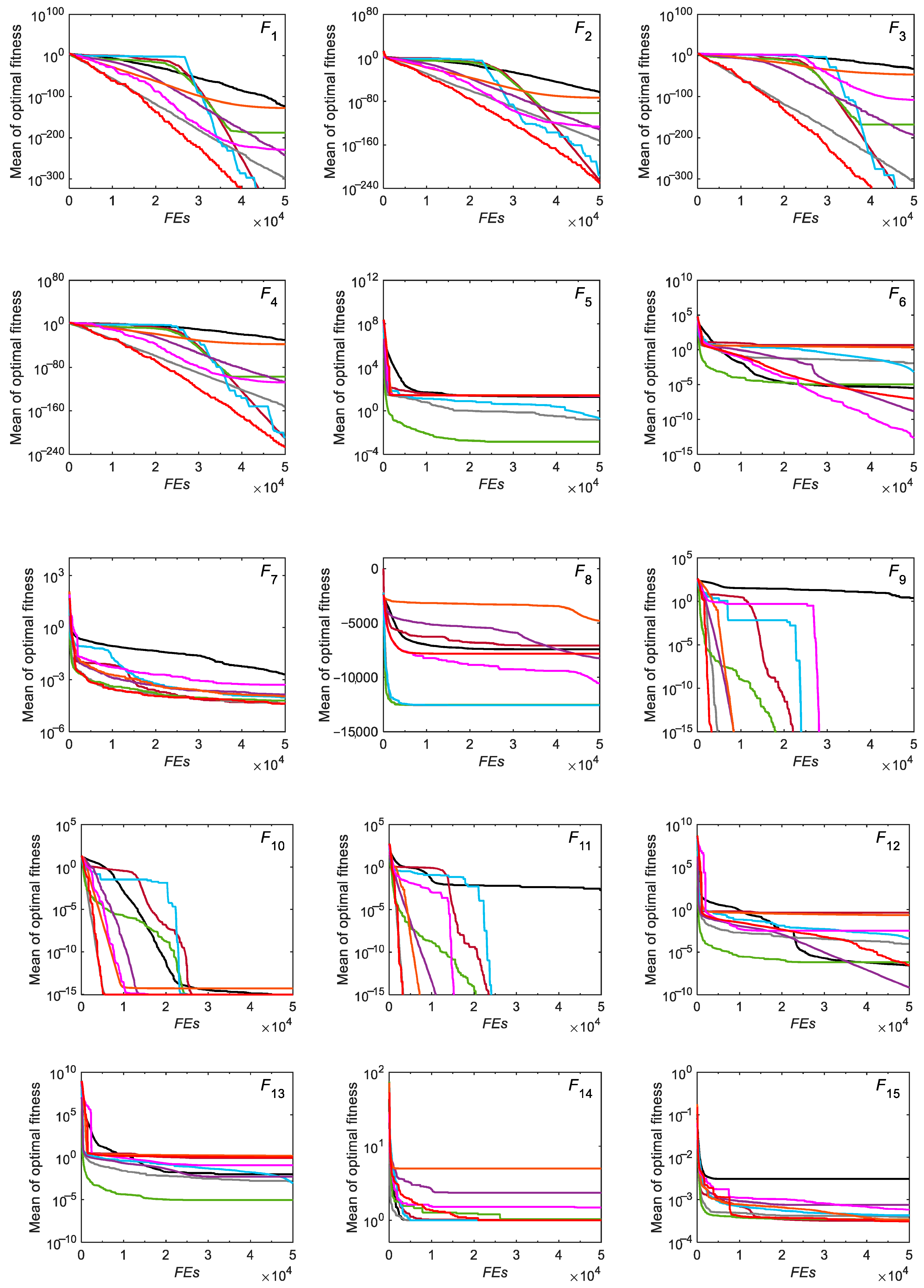
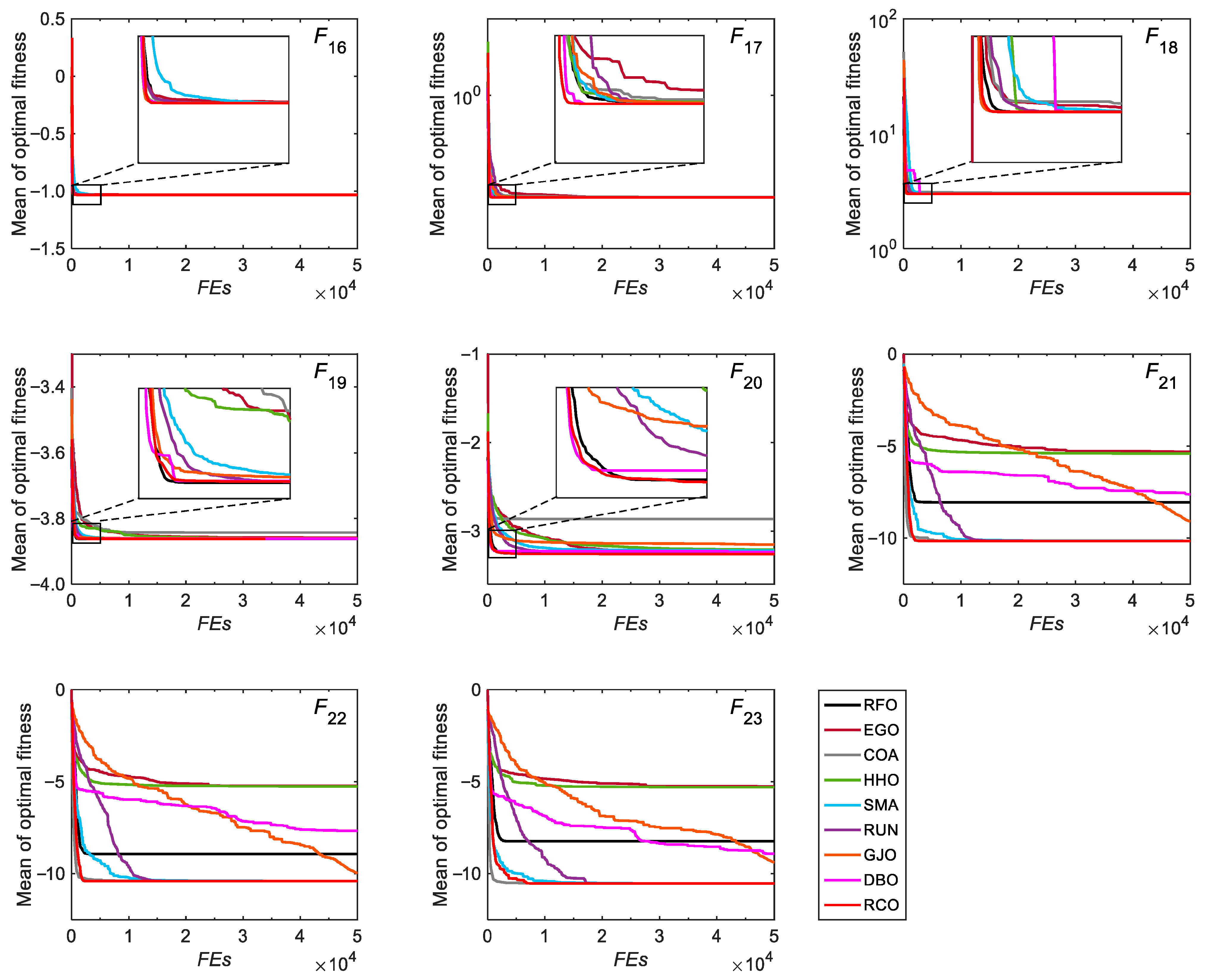
- The RCO algorithm is tested on CEC-2005 and CEC-2022 benchmark functions and is compared with eight popular algorithms from multiple perspectives, including optimization accuracy, convergence speed, rank-sum test, and scalability.
- The RCO algorithm is used to optimize eight constrained application problems, and the ability of the RCO algorithm to deal with engineering design problems is compared with fifteen other optimization algorithms.
2. Red-Crowned Crane Optimization (RCO)
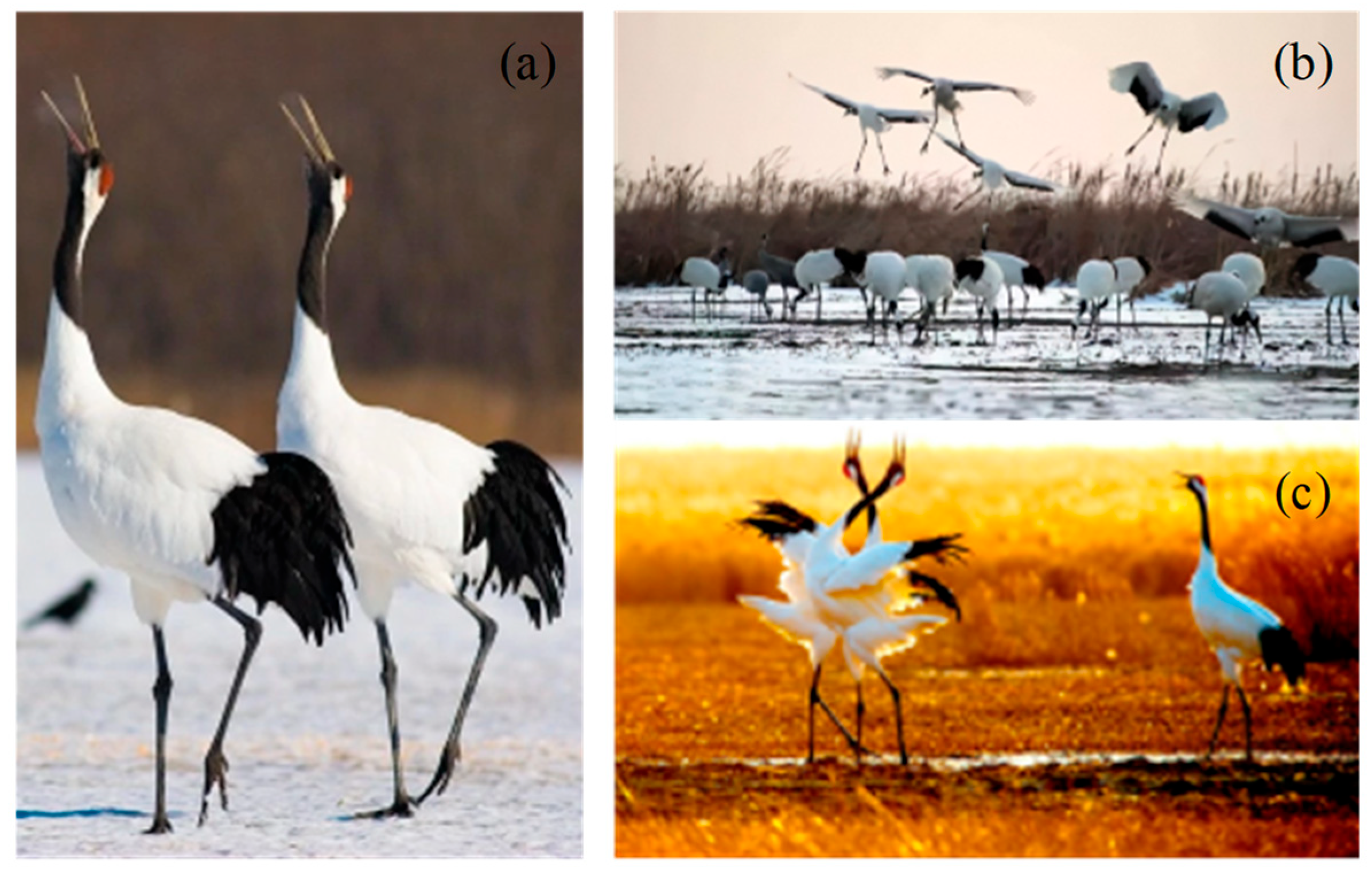
2.1. Inspiration Source
2.2. Population Initialization
2.3. Mathematical Model of RCO
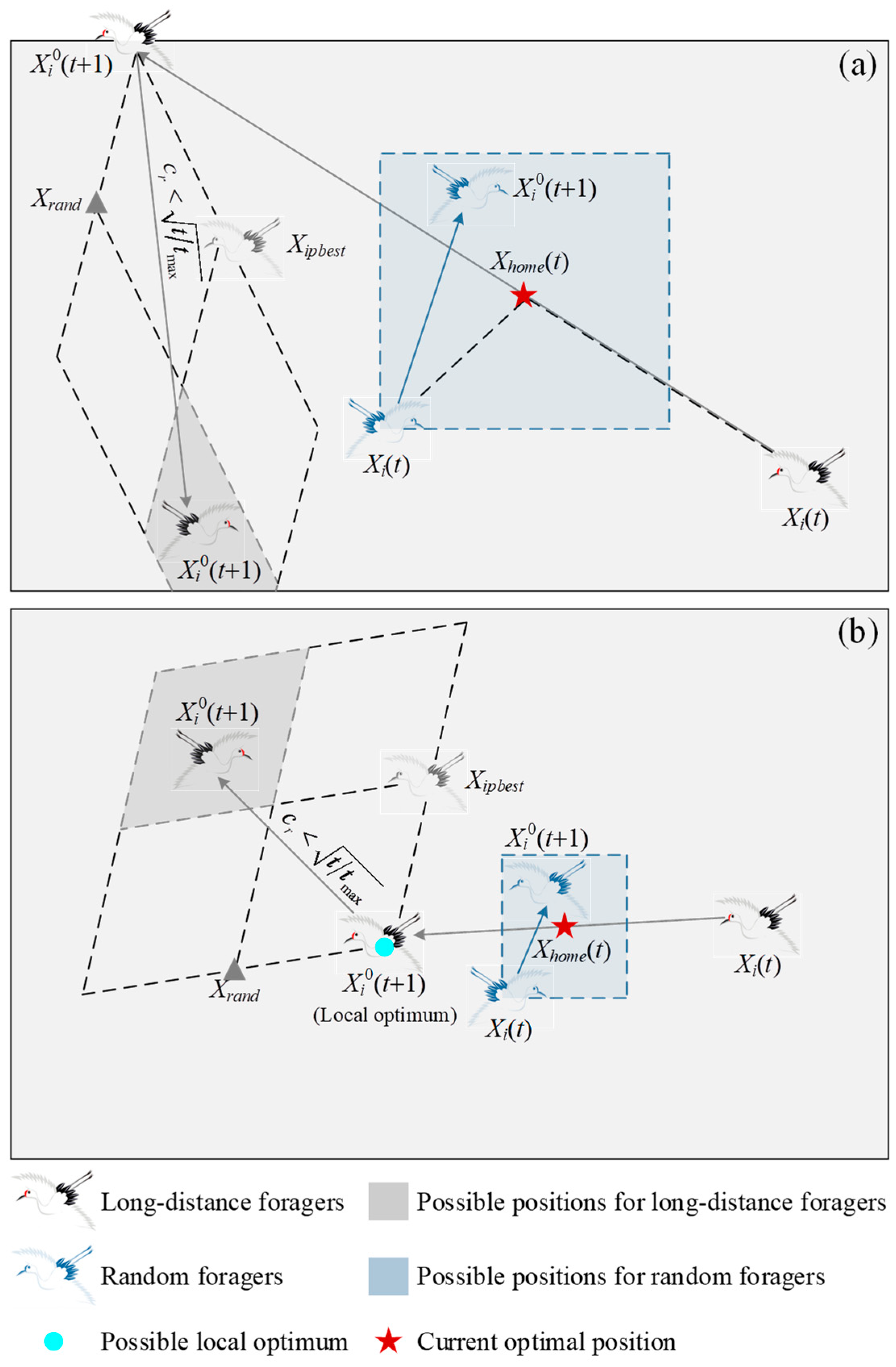
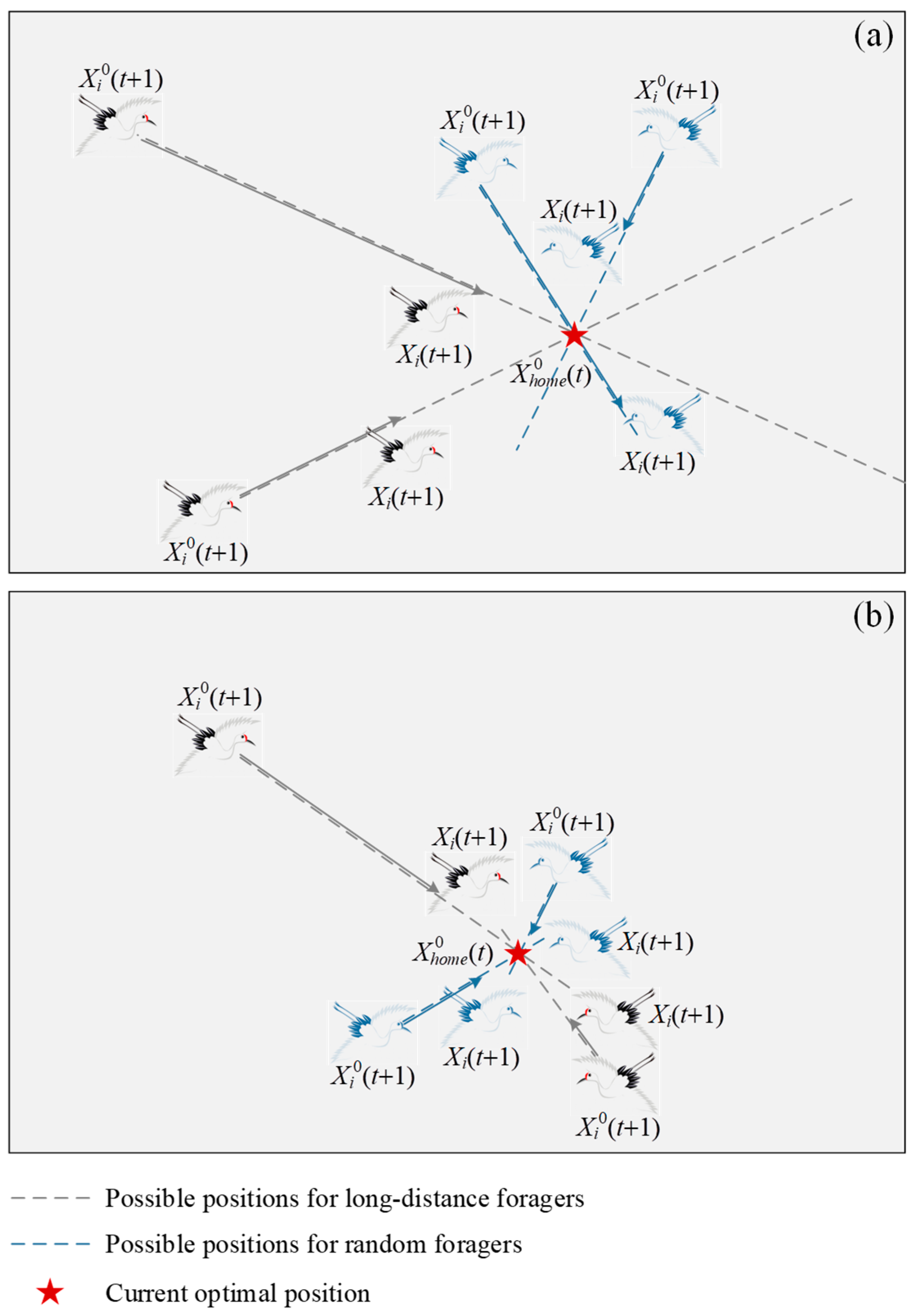
- Dispersing for foraging: The first thing to be pointed out is that the best position discovered by red-crowned cranes in the current iteration is considered an ideal habitat. Then, when daylight comes, the red-crowned cranes disperse from this habitat in search of food. They can be divided into two categories. Some red-crowned cranes forage randomly around the habitat, which are known as random foragers. Others have the courage to fly away from the habitat to explore richer food. These red-crowned cranes are called long-distance foragers.
- Avoiding danger: For the long-distance foragers, they usually live on the edge of the population and are more likely to be exposed to danger. Therefore, these red-crowned cranes are very alert when foraging for food. As soon as danger is imminent, they emit a ‘ko-lo-lo-’ call and take to the air to escape from the danger.
- Gathering for roosting: When the red-crowned cranes forage during the day, they also consider choosing a better habitat. If one red-crowned crane reaches a better position, this position will become a new habitat. At night, with the guidance of this red-crowned crane, other red-crowned cranes gather towards the new habitat.
- Crane dance: With certain probability, a male red-crowned crane and a female red-crowned crane can successfully pair up and express their love for each other through singing, jumping, and dancing. During this time, they sing and make loud sounds. As a result, other red-crowned cranes stop near them to enjoy their dance. In this case, the two red-crowned cranes with the first and second fitness values are considered this pair of red-crowned cranes.
2.3.1. Strategies Based on Foraging and Roosting Behaviors
2.3.2. Strategy Based on Crane Dance
2.4. Implementation of RCO
| Algorithm 1: Pseudo-code of RCO |
| Input: The maximum number of iterations tmax, the maximum number of function evaluations FEmax, the population size n, the probability coefficient pc, and the ratio of random foragers to long-distance foragers k:(n-k); Output: The best solution Xbest and its fitness value F(Xbest). 1: Initialize the red-crowned cranes Xcranes using Equations (1) and (2) 2: t = 0 and FEs = 0 3: while (t < tmax or FEs < FEmax) 4: Calculate the fitness values of all red-crowned cranes using Equation (3) 5: Record the first and second individuals so far 6: if r5 < pc 7: Take the position corresponding to the first fitness value as Xhome 8: Sort the red-crowned cranes according to their fitness values 9: for i = F1:Fk /Foraging behavior of random foragers/ 10: Update the positions of the random foragers using Equation (6) 11: Calculate the fitness values of random foragers 12: end for 13: for i = F(k+1):Fn /Foraging behavior of long-distance foragers/ 14: Update the positions of the long-distance foragers using Equation (7) 15: if cr < (t/tmax)1/2 /Escaping behavior of long-distance foragers/ 16: Generate Xrand and record Xipbest of long-distance foragers 17: Further update their positions using Equation (8) 18: end if 19: Calculate the fitness values of long-distance foragers 20: end for 21: Determine Xhome by comparing the fitness values of all red-crowned cranes after foraging with the fitness values of Xhome 22: for i = 1:n /Roosting behavior of red-crowned cranes/ 23: Update the positions of all red-crowned cranes using Equation (9) 24: end for 25: FEs = FEs + 2n 26: else 27: for i = 1:n /Crane dance of red-crowned cranes/ 28: Update the positions of red-crowned cranes using Equation (12) 29: end for 30: FEs = FEs + n 31: end if 32: t = t + 1 33: end while 34: Return Xbest and F(Xbest) |
2.5. Computational Complexity of RCO
3. Experimental Results and Discussion
3.1. Experimental Setup
3.2. Tests on CEC-2005 Benchmark Functions
3.2.1. Exploitation and Exploration Analysis
3.2.2. Convergence Analysis
3.2.3. Non-Parametric Statistical Analysis
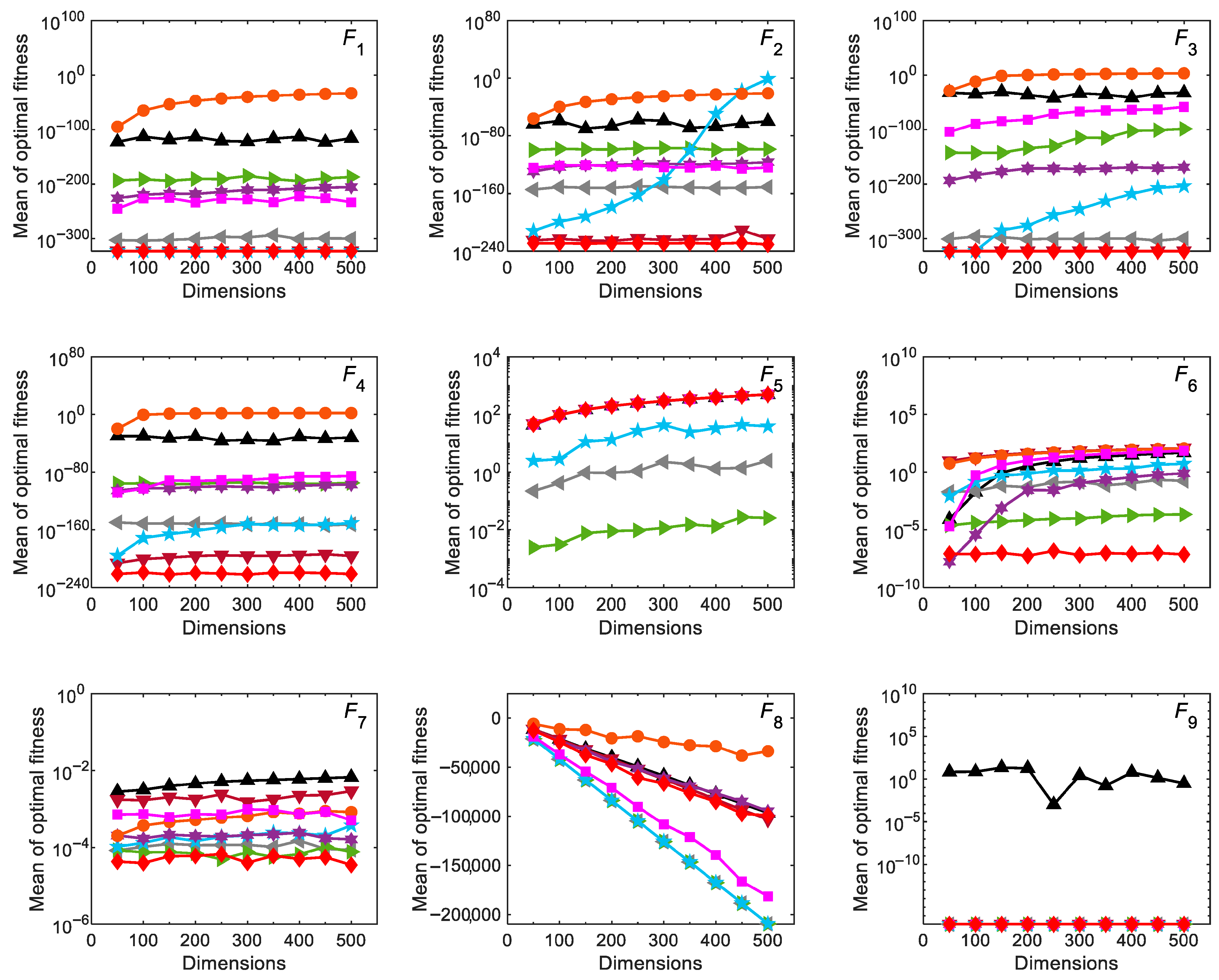
3.2.4. Scalability Analysis
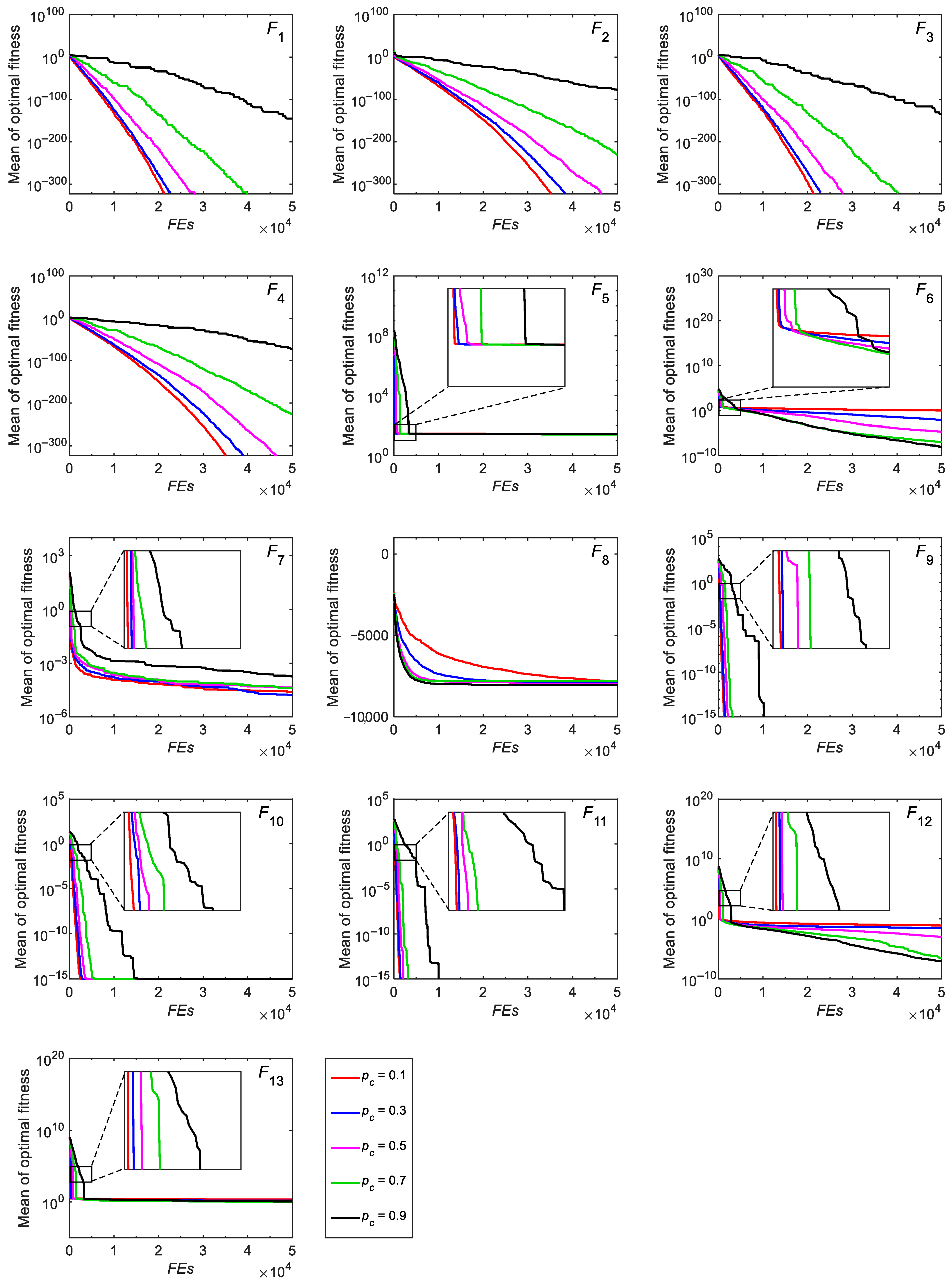
3.2.5. Parameter Analysis
3.2.6. Running Time Comparison
3.3. Tests on CEC-2022 Functions
4. Application of RCO in Engineering Design Problems
4.1. Constraint Handling Method
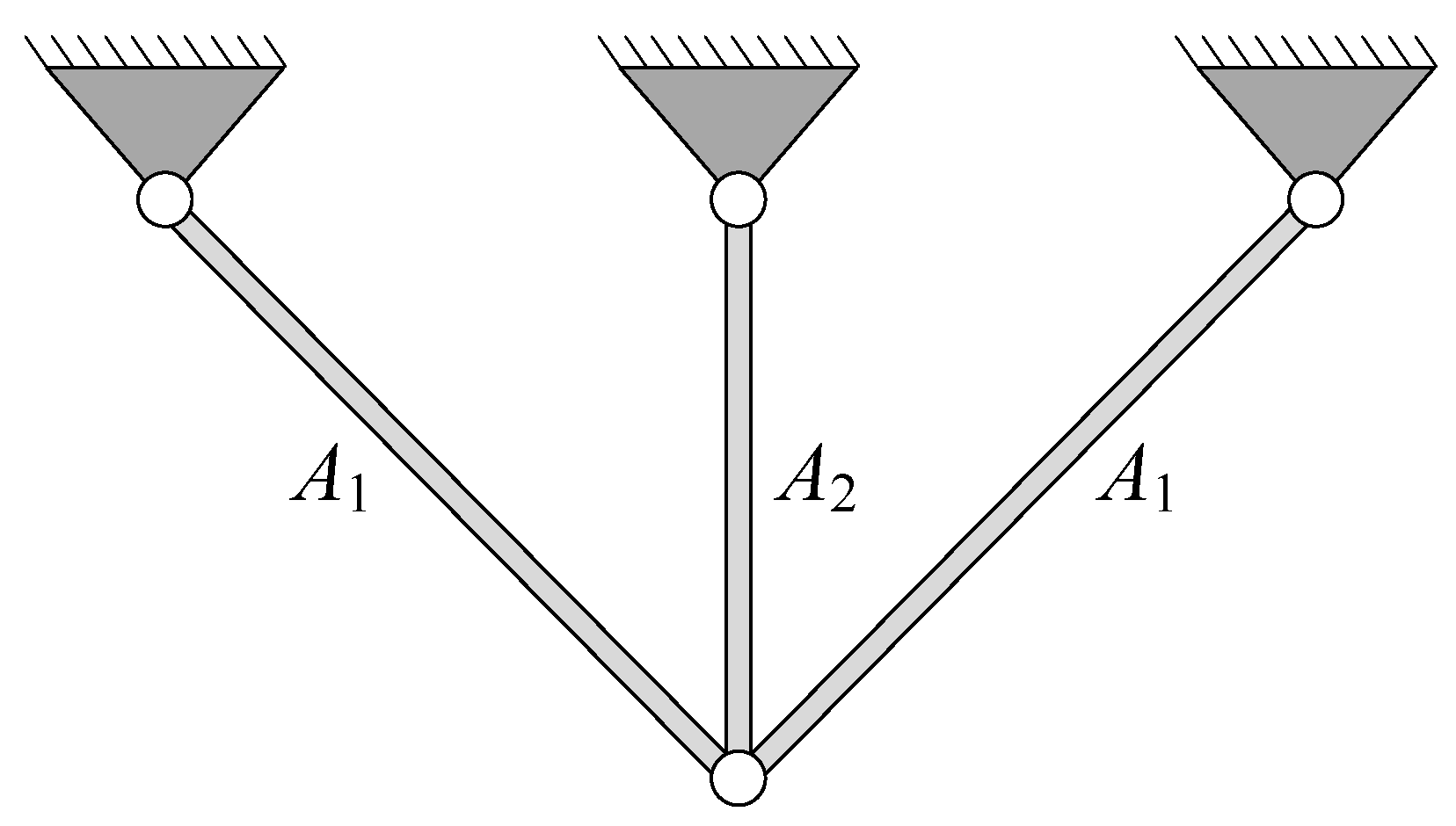
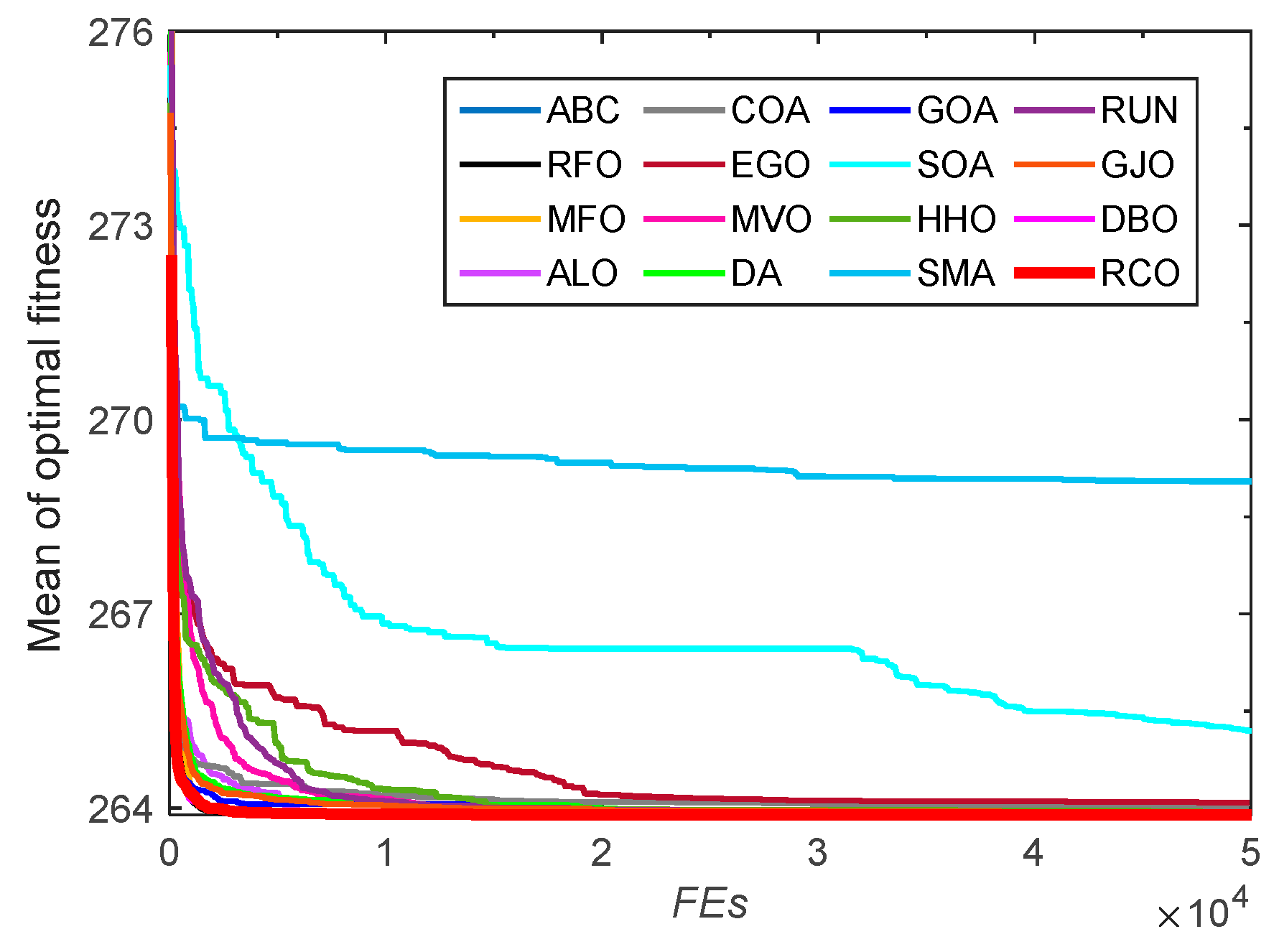
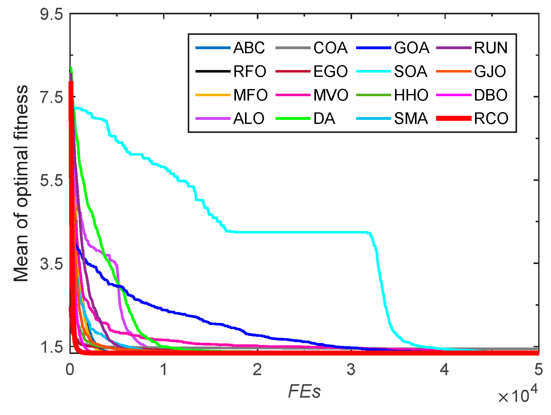
4.2. Three-Bar Truss Design Problem
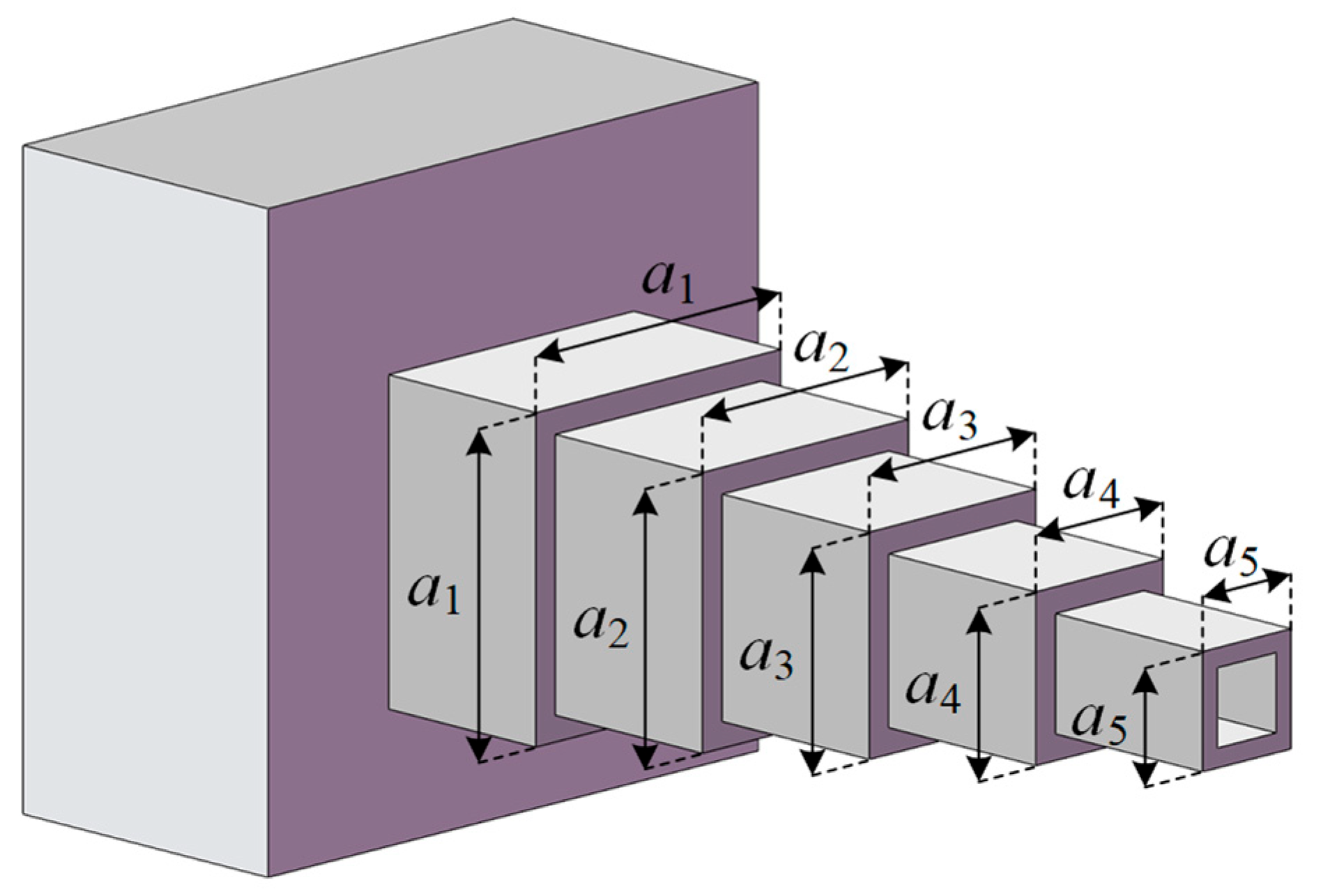
4.3. Cantilever Beam Design Problem
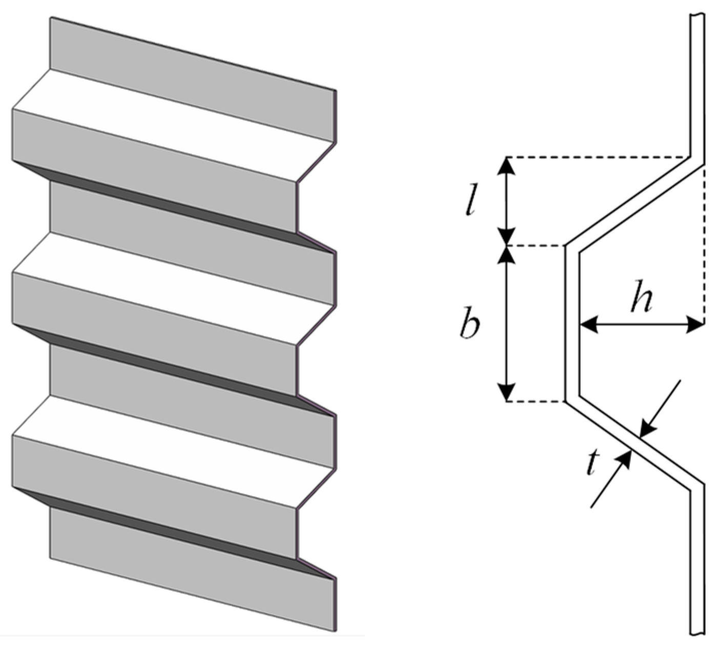
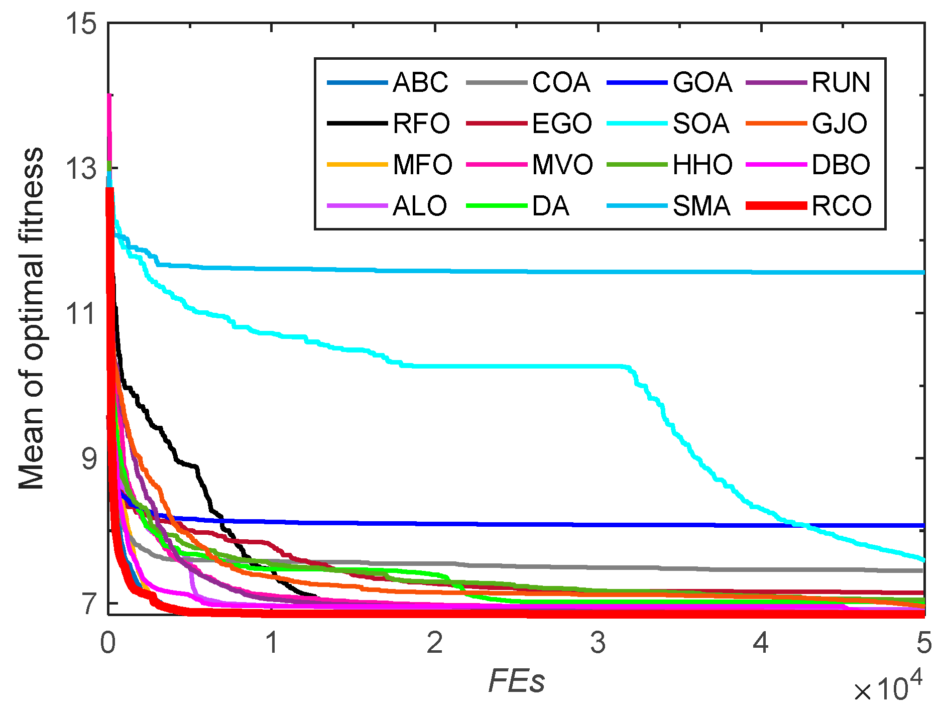
4.4. Corrugated Bulkhead Design Problem
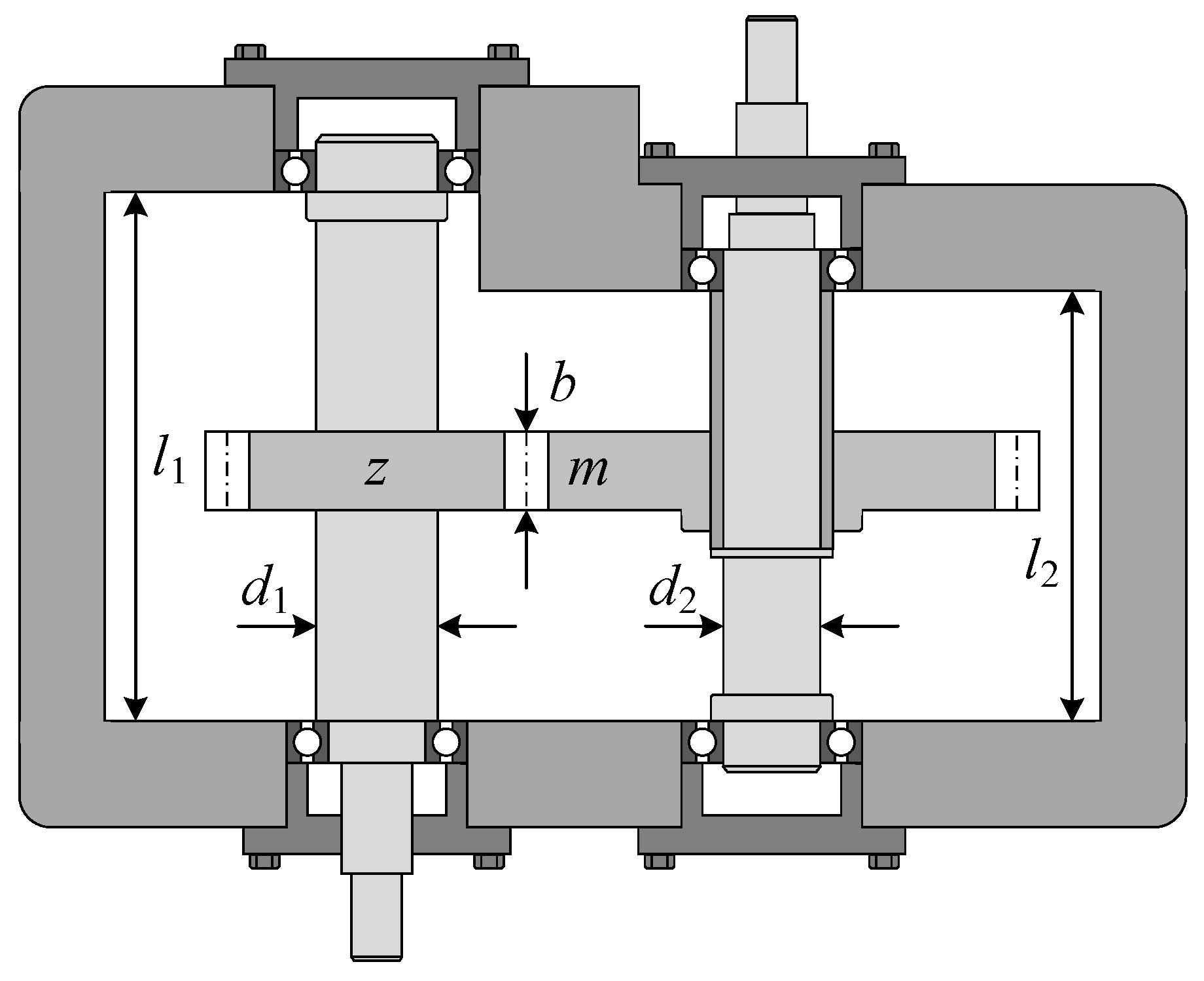
4.5. Speed Reducer Design Problem
5. Conclusions
Author Contributions
Funding
Data Availability Statement
Conflicts of Interest
Appendix A
| Index | RCO | DBO | GJO | RUN | SMA | HHO | COA | EGO | RFO | |
|---|---|---|---|---|---|---|---|---|---|---|
| F1 | Mean | 0 | 5.2809 × 10−230 | 3.9820 × 10−128 | 2.2935 × 10−243 | 0 | 1.0477 × 10−188 | 2.7846 × 10−300 | 0 | 1.9440 × 10−123 |
| Std | 0 | 2.8925 × 10−229 | 1.0427 × 10−127 | 7.3031 × 10−243 | 0 | 5.7385 × 10−188 | 1.5252 × 10−299 | 0 | 8.6274 × 10−123 | |
| Min | 0 | 0 | 1.9033 × 10−132 | 1.3587 × 10−264 | 0 | 1.1141 × 10−218 | 4.4465 × 10−323 | 0 | 9.2003 × 10−147 | |
| Max | 0 | 1.5843 × 10−228 | 4.1799 × 10−127 | 2.8536 × 10−242 | 0 | 3.1431 × 10−187 | 8.3539 × 10−299 | 0 | 4.7129 × 10−122 | |
| Rank | 1 | 6 | 8 | 5 | 1 | 7 | 4 | 1 | 9 | |
| F2 | Mean | 1.9434 × 10−238 | 2.3225 × 10−127 | 5.2171 × 10−74 | 1.3440 × 10−132 | 1.4401 × 10−216 | 3.6619 × 10−102 | 7.2913 × 10−153 | 6.5602 × 10−226 | 3.0528 × 10−64 |
| Std | 1.0645 × 10−237 | 1.2649 × 10−126 | 1.3483 × 10−73 | 5.4701 × 10−132 | 7.8877 × 10−216 | 1.1524 × 10−101 | 2.4693 × 10−152 | 2.0974 × 10−225 | 1.0288 × 10−63 | |
| Min | 3.5173 × 10−289 | 1.8746 × 10−155 | 9.6739 × 10−76 | 1.1056 × 10−144 | 0 | 1.7402 × 10−115 | 1.7869 × 10−161 | 2.6197 × 10−235 | 3.0543 × 10−78 | |
| Max | 5.8303 × 10−237 | 6.9297 × 10−126 | 5.5034 × 10−73 | 2.9423 × 10−131 | 4.3203 × 10−215 | 6.0460 × 10−101 | 1.1194 × 10−151 | 9.1667 × 10−225 | 5.0084 × 10−63 | |
| Rank | 1 | 6 | 8 | 5 | 3 | 7 | 4 | 2 | 9 | |
| F3 | Mean | 0 | 1.2452 × 10−108 | 1.1524 × 10−46 | 2.9380 × 10−203 | 0 | 1.4027 × 10−168 | 1.4690 × 10−306 | 0 | 7.8981 × 10⁻³³ |
| Std | 0 | 6.8205 × 10−108 | 5.9207 × 10−46 | 1.6092 × 10−202 | 0 | 7.6814 × 10−168 | 5.5447 × 10−306 | 0 | 4.3252 × 10⁻³² | |
| Min | 0 | 8.7993 × 10−296 | 1.2082 × 10−55 | 5.9121 × 10−231 | 0 | 1.5541 × 10−191 | 5.4347 × 10−322 | 0 | 6.7212 × 10−52 | |
| Max | 0 | 3.7357 × 10−107 | 3.2464 × 10−45 | 8.8141 × 10−202 | 0 | 4.2073 × 10−167 | 2.5106 × 10−305 | 0 | 2.3690 × 10⁻³¹ | |
| Rank | 1 | 7 | 8 | 5 | 1 | 6 | 4 | 1 | 9 | |
| F4 | Mean | 1.3051 × 10−226 | 1.2965 × 10−108 | 1.4151 × 10−38 | 2.2911 × 10−107 | 2.4594 × 10−209 | 5.4802 × 10−98 | 3.4686 × 10−153 | 1.2982 × 10−210 | 1.2699 × 10⁻³⁰ |
| Std | 7.1478 × 10−226 | 7.1009 × 10−108 | 3.9775 × 10−38 | 1.2446 × 10−106 | 1.3471 × 10−208 | 1.5566 × 10−97 | 8.2139 × 10−153 | 6.0192 × 10−210 | 6.7899 × 10⁻³⁰ | |
| Min | 1.8275 × 10−279 | 8.3784 × 10−157 | 4.6046 × 10−41 | 1.9124 × 10−124 | 0 | 6.2512 × 10−110 | 1.7214 × 10−161 | 1.3882 × 10−224 | 7.4726 × 10−49 | |
| Max | 3.9150 × 10−225 | 3.8893 × 10−107 | 2.1602 × 10−37 | 6.8188 × 10−106 | 7.3783 × 10−208 | 8.2062 × 10−97 | 2.8000 × 10−152 | 3.2877 × 10−209 | 3.7211 × 10⁻²⁹ | |
| Rank | 1 | 5 | 8 | 6 | 3 | 7 | 4 | 2 | 9 | |
| F5 | Mean | 2.3255 × 101 | 2.4222 × 101 | 2.7537 × 101 | 2.3002 × 101 | 1.6940 × 10⁻¹ | 1.4904 × 10⁻³ | 1.4705 × 10⁻¹ | 2.7439 × 101 | 1.9529 × 101 |
| Std | 1.3112 × 10⁻¹ | 2.0856 × 10⁻¹ | 8.1310 × 10⁻¹ | 1.2877 × 100 | 1.3180 × 10⁻¹ | 2.8720 × 10⁻³ | 2.4898 × 10⁻¹ | 6.2131 × 10⁻¹ | 3.0118 × 100 | |
| Min | 2.2954 × 101 | 2.3818 × 101 | 2.6218 × 101 | 2.0991 × 101 | 3.3788 × 10⁻³ | 1.9144 × 10⁻⁶ | 3.3091 × 10⁻³ | 2.6492 × 101 | 4.1507 × 100 | |
| Max | 2.3553 × 101 | 2.4549 × 101 | 2.8830 × 101 | 2.5741 × 101 | 4.7196 × 10⁻¹ | 1.5115 × 10⁻² | 1.3118 × 100 | 2.8745 × 101 | 2.3250 × 101 | |
| Rank | 6 | 7 | 9 | 5 | 3 | 1 | 2 | 8 | 4 | |
| F6 | Mean | 8.2703 × 10⁻⁸ | 2.2893 × 10⁻¹³ | 2.2185 × 100 | 1.5362 × 10⁻⁹ | 6.9817 × 10⁻⁴ | 1.1121 × 10⁻⁵ | 1.2516 × 10⁻² | 4.6390 × 100 | 3.5866 × 10⁻⁶ |
| Std | 8.8799 × 10⁻⁸ | 7.0206 × 10⁻¹³ | 4.9214 × 10⁻¹ | 6.2534 × 10⁻¹⁰ | 3.0287 × 10⁻⁴ | 1.5140 × 10⁻⁵ | 1.3605 × 10⁻² | 4.0602 × 10⁻¹ | 2.2533 × 10⁻⁶ | |
| Min | 3.5588 × 10⁻⁹ | 1.0557 × 10⁻¹⁵ | 1.2516 × 100 | 6.0582 × 10⁻¹⁰ | 3.0562 × 10⁻⁴ | 2.2074 × 10⁻⁸ | 1.4359 × 10⁻⁴ | 3.8596 × 100 | 8.2509 × 10⁻⁷ | |
| Max | 3.2621 × 10⁻⁷ | 2.9547 × 10⁻¹² | 3.5005 × 100 | 3.7636 × 10⁻⁹ | 1.3765 × 10⁻³ | 6.7073 × 10⁻⁵ | 4.4397 × 10⁻² | 5.3294 × 100 | 8.4035 × 10⁻⁶ | |
| Rank | 3 | 1 | 8 | 2 | 6 | 5 | 7 | 9 | 4 | |
| F7 | Mean | 3.8235 × 10⁻⁵ | 4.9274 × 10⁻⁴ | 1.0833 × 10⁻⁴ | 1.3639 × 10⁻⁴ | 9.4520 × 10⁻⁵ | 6.1586 × 10⁻⁵ | 3.9921 × 10⁻⁵ | 3.9288 × 10⁻⁵ | 1.9593 × 10⁻³ |
| Std | 5.4596 × 10⁻⁵ | 4.1904 × 10⁻⁴ | 9.5409 × 10⁻⁵ | 8.4876 × 10⁻⁵ | 1.1986 × 10⁻⁴ | 8.2083 × 10⁻⁵ | 2.7439 × 10⁻⁵ | 2.7069 × 10⁻⁵ | 2.1825 × 10⁻³ | |
| Min | 5.4448 × 10⁻⁷ | 4.2673 × 10⁻⁵ | 8.5343 × 10⁻⁶ | 2.2017 × 10⁻⁵ | 4.8300 × 10⁻⁶ | 1.6027 × 10⁻⁶ | 7.4315 × 10⁻⁷ | 3.5073 × 10⁻⁶ | 1.1118 × 10⁻⁴ | |
| Max | 2.8157 × 10⁻⁴ | 1.5603 × 10⁻³ | 3.7173 × 10⁻⁴ | 3.8663 × 10⁻⁴ | 6.3406 × 10⁻⁴ | 3.6845 × 10⁻⁴ | 1.0214 × 10⁻⁴ | 9.0637 × 10⁻⁵ | 9.0398 × 10⁻³ | |
| Rank | 1 | 8 | 6 | 7 | 5 | 4 | 3 | 2 | 9 | |
| F8 | Mean | −7.8058 × 10³ | −1.0527 × 10⁴ | −4.7758 × 10³ | −8.3556 × 10³ | −1.2569 × 10⁴ | −1.2530 × 10⁴ | −1.2569 × 10⁴ | −7.0586 × 10³ | −7.4069 × 10³ |
| Std | 1.1148 × 10³ | 1.9844 × 10³ | 1.0318 × 10³ | 5.9000 × 10² | 3.0944 × 10⁻² | 2.1715 × 10² | 2.8011 × 10⁻² | 9.2974 × 10² | 9.1907 × 10² | |
| Min | −1.1403 × 10⁴ | −1.2562 × 10⁴ | −6.5500 × 10³ | −9.4898 × 10³ | −1.2569 × 10⁴ | −1.2569 × 10⁴ | −1.2569 × 10⁴ | −9.3321 × 10³ | −9.5175 × 10³ | |
| Max | −6.5455 × 10³ | −6.8480 × 10³ | −3.0756 × 10³ | −6.9719 × 10³ | −1.2569 × 10⁴ | −1.1380 × 10⁴ | −1.2569 × 10⁴ | −5.8874 × 10³ | −5.8374 × 10³ | |
| Rank | 6 | 4 | 9 | 5 | 2 | 3 | 1 | 8 | 7 | |
| F9 | Mean | 0 | 0 | 0 | 0 | 0 | 0 | 0 | 0 | 2.4215 × 100 |
| Std | 0 | 0 | 0 | 0 | 0 | 0 | 0 | 0 | 9.2071 × 100 | |
| Min | 0 | 0 | 0 | 0 | 0 | 0 | 0 | 0 | 0 | |
| Max | 0 | 0 | 0 | 0 | 0 | 0 | 0 | 0 | 4.5768 × 101 | |
| Rank | 1 | 1 | 1 | 1 | 1 | 1 | 1 | 1 | 9 | |
| F10 | Mean | 8.8818 × 10⁻¹⁶ | 8.8818 × 10⁻¹⁶ | 4.6777 × 10⁻¹⁵ | 8.8818 × 10⁻¹⁶ | 8.8818 × 10⁻¹⁶ | 8.8818 × 10⁻¹⁶ | 8.8818 × 10⁻¹⁶ | 8.8818 × 10⁻¹⁶ | 8.8818 × 10⁻¹⁶ |
| Std | 0 | 0 | 9.0135 × 10⁻¹⁶ | 0 | 0 | 0 | 0 | 0 | 0 | |
| Min | 8.8818 × 10⁻¹⁶ | 8.8818 × 10⁻¹⁶ | 4.4409 × 10⁻¹⁵ | 8.8818 × 10⁻¹⁶ | 8.8818 × 10⁻¹⁶ | 8.8818 × 10⁻¹⁶ | 8.8818 × 10⁻¹⁶ | 8.8818 × 10⁻¹⁶ | 8.8818 × 10⁻¹⁶ | |
| Max | 8.8818 × 10⁻¹⁶ | 8.8818 × 10⁻¹⁶ | 7.9936 × 10⁻¹⁵ | 8.8818 × 10⁻¹⁶ | 8.8818 × 10⁻¹⁶ | 8.8818 × 10⁻¹⁶ | 8.8818 × 10⁻¹⁶ | 8.8818 × 10⁻¹⁶ | 8.8818 × 10⁻¹⁶ | |
| Rank | 1 | 1 | 9 | 1 | 1 | 1 | 1 | 1 | 1 | |
| F11 | Mean | 0 | 0 | 0 | 0 | 0 | 0 | 0 | 0 | 2.0490 × 10⁻³ |
| Std | 0 | 0 | 0 | 0 | 0 | 0 | 0 | 0 | 9.1755 × 10⁻³ | |
| Min | 0 | 0 | 0 | 0 | 0 | 0 | 0 | 0 | 0 | |
| Max | 0 | 0 | 0 | 0 | 0 | 0 | 0 | 0 | 4.9149 × 10⁻² | |
| Rank | 1 | 1 | 1 | 1 | 1 | 1 | 1 | 1 | 9 | |
| F12 | Mean | 2.1603 × 10⁻⁷ | 3.4556 × 10⁻³ | 2.3100 × 10⁻¹ | 6.7256 × 10⁻¹⁰ | 3.9651 × 10⁻⁴ | 6.6063 × 10⁻⁷ | 9.6963 × 10⁻⁵ | 4.5220 × 10⁻¹ | 2.6797 × 10⁻⁷ |
| Std | 4.7274 × 10⁻⁷ | 1.8927 × 10⁻² | 1.7503 × 10⁻¹ | 1.9651 × 10⁻¹⁰ | 5.9390 × 10⁻⁴ | 8.9000 × 10⁻⁷ | 1.2439 × 10⁻⁴ | 7.9334 × 10⁻² | 1.7045 × 10⁻⁷ | |
| Min | 1.2207 × 10⁻⁸ | 1.5935 × 10⁻¹⁷ | 9.9289 × 10⁻² | 4.0781 × 10⁻¹⁰ | 1.2079 × 10⁻⁶ | 1.4431 × 10⁻⁸ | 1.7254 × 10⁻⁷ | 2.9122 × 10⁻¹ | 7.2406 × 10⁻⁸ | |
| Max | 2.5373 × 10⁻⁶ | 1.0367 × 10⁻¹ | 7.9104 × 10⁻¹ | 1.2067 × 10⁻⁹ | 2.9710 × 10⁻³ | 4.0629 × 10⁻⁶ | 4.9112 × 10⁻⁴ | 6.3744 × 10⁻¹ | 7.9917 × 10⁻⁷ | |
| Rank | 2 | 7 | 8 | 1 | 6 | 4 | 5 | 9 | 3 | |
| F13 | Mean | 9.7940 × 10⁻¹ | 1.1682 × 10⁻¹ | 1.4702 × 100 | 5.0640 × 10⁻³ | 8.8519 × 10⁻⁴ | 9.0349 × 10⁻⁶ | 1.4980 × 10⁻³ | 7.9877 × 10⁻¹ | 9.8447 × 10⁻³ |
| Std | 7.1097 × 10⁻¹ | 1.4208 × 10⁻¹ | 2.5182 × 10⁻¹ | 6.7515 × 10⁻³ | 2.0406 × 10⁻³ | 1.6272 × 10⁻⁵ | 2.4410 × 10⁻³ | 3.5452 × 10⁻¹ | 3.0028 × 10⁻² | |
| Min | 2.4881 × 10⁻⁵ | 4.6345 × 10⁻¹⁵ | 8.4171 × 10⁻¹ | 2.2125 × 10⁻⁹ | 4.2916 × 10⁻⁵ | 5.8846 × 10⁻⁸ | 4.2391 × 10⁻⁶ | 3.1981 × 10⁻¹ | 9.5356 × 10⁻⁷ | |
| Max | 2.7692 × 100 | 6.0266 × 10⁻¹ | 1.9765 × 100 | 2.1024 × 10⁻² | 1.1598 × 10⁻² | 8.0253 × 10⁻⁵ | 1.2578 × 10⁻² | 1.7298 × 100 | 9.8924 × 10⁻² | |
| Rank | 8 | 6 | 9 | 4 | 2 | 1 | 3 | 7 | 5 | |
| F14 | Mean | 9.9800 × 10⁻¹ | 1.4887 × 100 | 4.9781 × 100 | 2.3436 × 100 | 9.9800 × 10⁻¹ | 1.0311 × 100 | 9.9800 × 10⁻¹ | 1.0118 × 100 | 9.9800 × 10⁻¹ |
| Std | 2.3142 × 10⁻¹⁶ | 1.8652 × 100 | 4.3820 × 100 | 2.4550 × 100 | 2.0785 × 10⁻¹⁴ | 1.8148 × 10⁻¹ | 4.9859 × 10⁻¹¹ | 5.1198 × 10⁻² | 4.1233 × 10⁻¹⁶ | |
| Min | 9.9800 × 10⁻¹ | 9.9800 × 10⁻¹ | 9.9800 × 10⁻¹ | 9.9800 × 10⁻¹ | 9.9800 × 10⁻¹ | 9.9800 × 10⁻¹ | 9.9800 × 10⁻¹ | 9.9800 × 10⁻¹ | 9.9800 × 10⁻¹ | |
| Max | 9.9800 × 10⁻¹ | 1.0763 × 101 | 1.2671 × 101 | 1.0763 × 101 | 9.9800 × 10⁻¹ | 1.9920 × 100 | 9.9800 × 10⁻¹ | 1.2798 × 100 | 9.9800 × 10⁻¹ | |
| Rank | 1 | 7 | 9 | 8 | 3 | 6 | 4 | 5 | 2 | |
| F15 | Mean | 3.2153 × 10⁻⁴ | 5.8790 × 10⁻⁴ | 3.4290 × 10⁻⁴ | 7.6533 × 10⁻⁴ | 4.3310 × 10⁻⁴ | 3.5002 × 10⁻⁴ | 3.9725 × 10⁻⁴ | 3.2385 × 10⁻⁴ | 3.1037 × 10⁻³ |
| Std | 3.5851 × 10⁻⁵ | 2.8511 × 10⁻⁴ | 1.6828 × 10⁻⁴ | 4.6567 × 10⁻⁴ | 2.0813 × 10⁻⁴ | 1.6951 × 10⁻⁴ | 1.0307 × 10⁻⁴ | 2.0846 × 10⁻⁵ | 6.8926 × 10⁻³ | |
| Min | 3.0749 × 10⁻⁴ | 3.0749 × 10⁻⁴ | 3.0749 × 10⁻⁴ | 3.0749 × 10⁻⁴ | 3.0762 × 10⁻⁴ | 3.0776 × 10⁻⁴ | 3.0995 × 10⁻⁴ | 3.0878 × 10⁻⁴ | 3.0749 × 10⁻⁴ | |
| Max | 4.3029 × 10⁻⁴ | 1.2239 × 10⁻³ | 1.2232 × 10⁻³ | 1.2232 × 10⁻³ | 1.2233 × 10⁻³ | 1.2437 × 10⁻³ | 6.7254 × 10⁻⁴ | 4.1770 × 10⁻⁴ | 2.0363 × 10⁻² | |
| Rank | 1 | 7 | 3 | 8 | 6 | 4 | 5 | 2 | 9 | |
| F16 | Mean | −1.0316 × 100 | −1.0316 × 100 | −1.0316 × 100 | −1.0316 × 100 | −1.0316 × 100 | −1.0316 × 100 | −1.0316 × 100 | −1.0310 × 100 | −1.0316 × 100 |
| Std | 5.3761 × 10⁻¹⁶ | 6.6486 × 10⁻¹⁶ | 1.8306 × 10⁻⁸ | 3.1600 × 10⁻¹³ | 1.2302 × 10⁻¹¹ | 1.7724 × 10⁻¹² | 1.4653 × 10⁻⁴ | 6.2720 × 10⁻⁴ | 6.7752 × 10⁻¹⁶ | |
| Min | −1.0316 × 100 | −1.0316 × 100 | −1.0316 × 100 | −1.0316 × 100 | −1.0316 × 100 | −1.0316 × 100 | −1.0316 × 100 | −1.0316 × 100 | −1.0316 × 100 | |
| Max | −1.0316 × 100 | −1.0316 × 100 | −1.0316 × 100 | −1.0316 × 100 | −1.0316 × 100 | −1.0316 × 100 | −1.0308 × 100 | −1.0293 × 100 | −1.0316 × 100 | |
| Rank | 1 | 2 | 7 | 4 | 6 | 5 | 8 | 9 | 3 | |
| F17 | Mean | 3.9789 × 10⁻¹ | 3.9789 × 10⁻¹ | 3.9789 × 10⁻¹ | 3.9789 × 10⁻¹ | 3.9789 × 10⁻¹ | 3.9789 × 10⁻¹ | 3.9829 × 10⁻¹ | 3.9909 × 10⁻¹ | 3.9789 × 10⁻¹ |
| Std | 0 | 0 | 6.5154 × 10⁻⁶ | 1.1965 × 10⁻¹¹ | 2.9134 × 10⁻⁹ | 9.3218 × 10⁻⁸ | 1.3177 × 10⁻³ | 5.3145 × 10⁻³ | 0 | |
| Min | 3.9789 × 10⁻¹ | 3.9789 × 10⁻¹ | 3.9789 × 10⁻¹ | 3.9789 × 10⁻¹ | 3.9789 × 10⁻¹ | 3.9789 × 10⁻¹ | 3.9789 × 10⁻¹ | 3.9789 × 10⁻¹ | 3.9789 × 10⁻¹ | |
| Max | 3.9789 × 10⁻¹ | 3.9789 × 10⁻¹ | 3.9791 × 10⁻¹ | 3.9789 × 10⁻¹ | 3.9789 × 10⁻¹ | 3.9789 × 10⁻¹ | 4.0455 × 10⁻¹ | 4.2717 × 10⁻¹ | 3.9789 × 10⁻¹ | |
| Rank | 1 | 1 | 7 | 4 | 5 | 6 | 8 | 9 | 1 | |
| F18 | Mean | 3.0000 × 100 | 3.0000 × 100 | 3.0000 × 100 | 3.0000 × 100 | 3.0000 × 100 | 3.0000 × 100 | 3.0417 × 100 | 3.0002 × 100 | 3.0000 × 100 |
| Std | 2.0534 × 10⁻¹⁵ | 4.6868 × 10⁻¹⁵ | 7.8820 × 10⁻⁷ | 2.5021 × 10⁻¹³ | 1.3151 × 10⁻¹¹ | 6.4462 × 10⁻⁹ | 1.3874 × 10⁻¹ | 4.7576 × 10⁻⁴ | 1.2934 × 10⁻¹⁵ | |
| Min | 3.0000 × 100 | 3.0000 × 100 | 3.0000 × 100 | 3.0000 × 100 | 3.0000 × 100 | 3.0000 × 100 | 3.0000 × 100 | 3.0000 × 100 | 3.0000 × 100 | |
| Max | 3.0000 × 100 | 3.0000 × 100 | 3.0000 × 100 | 3.0000 × 100 | 3.0000 × 100 | 3.0000 × 100 | 3.7212 × 100 | 3.0021 × 100 | 3.0000 × 100 | |
| Rank | 2 | 3 | 7 | 4 | 5 | 6 | 9 | 8 | 1 | |
| F19 | Mean | −3.8628 × 100 | −3.8615 × 100 | −3.8612 × 100 | −3.8628 × 100 | −3.8628 × 100 | −3.8624 × 100 | −3.8430 × 100 | −3.8591 × 100 | −3.8628 × 100 |
| Std | 2.2494 × 10⁻¹⁵ | 2.9649 × 10⁻³ | 3.1976 × 10⁻³ | 3.1487 × 10⁻¹⁰ | 1.0144 × 10⁻⁸ | 6.4592 × 10⁻⁴ | 2.5786 × 10⁻² | 2.9782 × 10⁻³ | 2.7101 × 10⁻¹⁵ | |
| Min | −3.8628 × 100 | −3.8628 × 100 | −3.8628 × 100 | −3.8628 × 100 | −3.8628 × 100 | −3.8628 × 100 | −3.8628 × 100 | −3.8625 × 100 | −3.8628 × 100 | |
| Max | −3.8628 × 100 | −3.8549 × 100 | −3.8549 × 100 | −3.8628 × 100 | −3.8628 × 100 | −3.8602 × 100 | −3.7757 × 100 | −3.8544 × 100 | −3.8628 × 100 | |
| Rank | 1 | 6 | 8 | 3 | 4 | 5 | 9 | 7 | 2 | |
| F20 | Mean | −3.2863 × 100 | −3.2362 × 100 | −3.1541 × 100 | −3.2507 × 100 | −3.2189 × 100 | −3.2101 × 100 | −2.8638 × 100 | −3.2469 × 100 | −3.2508 × 100 |
| Std | 5.5415 × 10⁻² | 8.4116 × 10⁻² | 1.3116 × 10⁻¹ | 5.9241 × 10⁻² | 4.1112 × 10⁻² | 6.5791 × 10⁻² | 2.6506 × 10⁻¹ | 8.9701 × 10⁻² | 5.9397 × 10⁻² | |
| Min | −3.3220 × 100 | −3.3220 × 100 | −3.3220 × 100 | −3.3220 × 100 | −3.3220 × 100 | −3.3172 × 100 | −3.2038 × 100 | −3.3133 × 100 | −3.3224 × 100 | |
| Max | −3.2031 × 100 | −3.0839 × 100 | −2.6381 × 100 | −3.2031 × 100 | −3.2027 × 100 | −3.0883 × 100 | −2.1416 × 100 | −3.0449 × 100 | −3.2032 × 100 | |
| Rank | 1 | 5 | 8 | 3 | 6 | 7 | 9 | 4 | 2 | |
| F21 | Mean | −1.0153 × 101 | −7.6162 × 100 | −9.0867 × 100 | −1.0153 × 101 | −1.0153 × 101 | −5.3899 × 100 | −1.0153 × 101 | −5.3010 × 100 | −8.0521 × 100 |
| Std | 6.1269 × 10⁻¹⁵ | 2.5802 × 100 | 2.1780 × 100 | 5.1533 × 10⁻¹⁰ | 6.3068 × 10⁻⁵ | 1.2815 × 100 | 1.1031 × 10⁻⁴ | 1.0508 × 100 | 2.8888 × 100 | |
| Min | −1.0153 × 101 | −1.0153 × 101 | −1.0153 × 101 | −1.0153 × 101 | −1.0153 × 101 | −1.0135 × 101 | −1.0153 × 101 | −9.8387 × 100 | −1.0153 × 101 | |
| Max | −1.0153 × 101 | −5.0551 × 100 | −3.5916 × 100 | −1.0153 × 101 | −1.0153 × 101 | −5.0476 × 100 | −1.0153 × 101 | −4.9663 × 100 | −2.6305 × 100 | |
| Rank | 1 | 7 | 5 | 2 | 3 | 8 | 4 | 9 | 6 | |
| F22 | Mean | −1.0403 × 101 | −7.6775 × 100 | −9.9734 × 100 | −1.0403 × 101 | −1.0403 × 101 | −5.2615 × 100 | −1.0403 × 101 | −5.2316 × 100 | −8.9356 × 100 |
| Std | 2.4240 × 10⁻¹⁵ | 2.8037 × 100 | 1.6514 × 100 | 4.0533 × 10⁻¹⁰ | 4.1346 × 10⁻⁵ | 9.6677 × 10⁻¹ | 9.3489 × 10⁻⁵ | 9.3835 × 10⁻¹ | 2.7659 × 100 | |
| Min | −1.0403 × 101 | −1.0403 × 101 | −1.0403 × 101 | −1.0403 × 101 | −1.0403 × 101 | −1.0380 × 101 | −1.0403 × 101 | −1.0199 × 101 | −1.0403 × 101 | |
| Max | −1.0403 × 101 | −2.7659 × 100 | −2.8676 × 100 | −1.0403 × 101 | −1.0403 × 101 | −5.0687 × 100 | −1.0402 × 101 | −5.0158 × 100 | −2.7519 × 100 | |
| Rank | 1 | 7 | 5 | 2 | 3 | 8 | 4 | 9 | 6 | |
| F23 | Mean | −1.0536 × 101 | −8.9233 × 100 | −9.3781 × 100 | −1.0536 × 101 | −1.0536 × 101 | −5.3034 × 100 | −1.0536 × 101 | −5.2654 × 100 | −8.2315 × 100 |
| Std | 4.6181 × 10⁻¹⁵ | 2.5060 × 100 | 2.6826 × 100 | 2.9870 × 10⁻¹⁰ | 3.5879 × 10⁻⁵ | 9.7000 × 10⁻¹ | 7.3804 × 10⁻⁵ | 8.5743 × 10⁻¹ | 3.3811 × 100 | |
| Min | −1.0536 × 101 | −1.0536 × 101 | −1.0536 × 101 | −1.0536 × 101 | −1.0536 × 101 | −1.0439 × 101 | −1.0536 × 101 | −9.8046 × 100 | −1.0536 × 101 | |
| Max | −1.0536 × 101 | −5.1285 × 100 | −2.4216 × 100 | −1.0536 × 101 | −1.0536 × 101 | −5.1086 × 100 | −1.0536 × 101 | −5.0699 × 100 | −2.4217 × 100 | |
| Rank | 1 | 6 | 5 | 2 | 3 | 8 | 4 | 9 | 7 | |
| Mean rank | 2.5000 | 5.3261 | 7.0870 | 4.2826 | 3.9783 | 5.2826 | 4.9783 | 5.8913 | 5.6739 | |
| Total rank | 1 | 6 | 9 | 3 | 2 | 5 | 4 | 8 | 7 | |
| RCO | DBO | GJO | RUN | SMA | HHO | COA | EGO | RFO | |
|---|---|---|---|---|---|---|---|---|---|
| F1 | 0.2193 | 0.2014 | 0.2639 | 1.1369 | 0.8407 | 0.2436 | 0.1278 | 0.1708 | 0.3725 |
| F2 | 0.2248 | 0.2036 | 0.2619 | 1.0974 | 0.7864 | 0.2292 | 0.1346 | 0.1895 | 0.3849 |
| F3 | 0.5951 | 0.5736 | 0.6648 | 1.7278 | 1.1698 | 1.1522 | 0.6970 | 0.5200 | 0.7107 |
| F4 | 0.2137 | 0.1979 | 0.2523 | 1.0689 | 0.7894 | 0.2804 | 0.1250 | 0.1648 | 0.3703 |
| F5 | 0.2560 | 0.2415 | 0.2989 | 1.1596 | 0.8604 | 0.4365 | 0.1901 | 0.2065 | 0.4073 |
| F6 | 0.2137 | 0.2070 | 0.2526 | 1.0572 | 0.8014 | 0.3303 | 0.1240 | 0.1776 | 0.3688 |
| F7 | 0.3947 | 0.3755 | 0.4437 | 1.3862 | 0.9758 | 0.6812 | 0.4043 | 0.3431 | 0.5414 |
| F8 | 0.2598 | 0.2659 | 0.3086 | 1.1745 | 0.8498 | 0.4571 | 0.1896 | 0.2086 | 0.3960 |
| F9 | 0.2386 | 0.2120 | 0.2674 | 1.1250 | 0.8085 | 0.3817 | 0.1579 | 0.1823 | 0.3984 |
| F10 | 0.2437 | 0.2220 | 0.2707 | 1.1269 | 0.8099 | 0.3928 | 0.1690 | 0.1983 | 0.4053 |
| F11 | 0.2707 | 0.2672 | 0.3163 | 1.1852 | 0.8394 | 0.4590 | 0.2190 | 0.2228 | 0.4342 |
| F12 | 0.7002 | 0.6956 | 0.8083 | 1.9595 | 1.3313 | 1.5442 | 0.9279 | 0.6701 | 0.8538 |
| F13 | 0.7121 | 0.7053 | 0.8029 | 1.9861 | 1.2753 | 1.5663 | 0.9374 | 0.6804 | 1.1196 |
| F14 | 1.0432 | 1.1472 | 1.0631 | 2.6387 | 1.3272 | 2.6602 | 1.5988 | 0.9993 | 1.2211 |
| F15 | 0.1188 | 0.1918 | 0.1538 | 0.9414 | 0.4131 | 0.2722 | 0.1372 | 0.0949 | 0.3190 |
| F16 | 0.1046 | 0.1737 | 0.1422 | 0.9128 | 0.3749 | 0.2630 | 0.1259 | 0.0855 | 0.3233 |
| F17 | 0.0901 | 0.1721 | 0.1323 | 0.8944 | 0.3612 | 0.2314 | 0.1006 | 0.0906 | 0.3102 |
| F18 | 0.0875 | 0.1585 | 0.1239 | 0.9066 | 0.3632 | 0.2248 | 0.0997 | 0.0705 | 0.3057 |
| F19 | 0.1249 | 0.2003 | 0.1657 | 0.9690 | 0.4027 | 0.3106 | 0.1541 | 0.1048 | 0.3318 |
| F20 | 0.1352 | 0.2021 | 0.1857 | 0.9752 | 0.4621 | 0.3217 | 0.1562 | 0.1138 | 0.3544 |
| F21 | 0.1321 | 0.2016 | 0.1694 | 1.0126 | 0.4204 | 0.3049 | 0.1503 | 0.1067 | 0.3338 |
| F22 | 0.1360 | 0.2137 | 0.1808 | 1.0024 | 0.4532 | 0.3254 | 0.1689 | 0.1192 | 0.3528 |
| F23 | 0.1473 | 0.2197 | 0.1942 | 1.0146 | 0.4502 | 0.3686 | 0.1908 | 0.1292 | 0.3616 |
| Index | RCO | DBO | GJO | RUN | SMA | HHO | COA | EGO | RFO | |
|---|---|---|---|---|---|---|---|---|---|---|
| F24 | Mean | 3.0000 × 10² | 3.0000 × 10² | 2.5036 × 10³ | 3.0000 × 10² | 3.0000 × 10² | 3.0066 × 10² | 4.6737 × 10² | 6.8079 × 10² | 3.1808 × 10² |
| Std | 9.5520 × 10⁻⁷ | 6.5870 × 10⁻³ | 2.1924 × 10³ | 1.1582 × 10⁻⁴ | 1.8839 × 10⁻⁴ | 2.6587 × 10⁻¹ | 6.7693 × 101 | 1.0234 × 10² | 4.9090 × 101 | |
| Min | 3.0000 × 10² | 3.0000 × 10² | 4.3993 × 10² | 3.0000 × 10² | 3.0000 × 10² | 3.0025 × 10² | 3.2378 × 10² | 4.8892 × 10² | 3.0000 × 10² | |
| Max | 3.0000 × 10² | 3.0004 × 10² | 8.5756 × 10³ | 3.0000 × 10² | 3.0000 × 10² | 3.0144 × 10² | 6.5187 × 10² | 8.7563 × 10² | 5.6092 × 10² | |
| Rank | 1 | 4 | 9 | 2 | 3 | 5 | 7 | 8 | 6 | |
| F25 | Mean | 4.0845 × 10² | 4.2628 × 10² | 4.4023 × 10² | 4.0961 × 10² | 4.0963 × 10² | 4.1502 × 10² | 4.3332 × 10² | 4.2556 × 10² | 4.0938 × 10² |
| Std | 1.3978 × 101 | 3.1933 × 101 | 2.8100 × 101 | 1.7157 × 101 | 1.2213 × 101 | 2.1922 × 101 | 3.0829 × 101 | 2.2737 × 101 | 4.4093 × 100 | |
| Min | 4.0000 × 10² | 4.0012 × 10² | 4.0644 × 10² | 4.0000 × 10² | 4.0564 × 10² | 4.0004 × 10² | 4.0020 × 10² | 4.0062 × 10² | 4.0014 × 10² | |
| Max | 4.6894 × 10² | 4.9270 × 10² | 5.2571 × 10² | 4.7078 × 10² | 4.7393 × 10² | 4.7104 × 10² | 4.8553 × 10² | 4.7090 × 10² | 4.1946 × 10² | |
| Rank | 1 | 7 | 9 | 3 | 4 | 5 | 8 | 6 | 2 | |
| F26 | Mean | 6.1579 × 10² | 6.2004 × 10² | 6.3574 × 10² | 6.1663 × 10² | 6.0007 × 10² | 6.2819 × 10² | 6.1631 × 10² | 6.1688 × 10² | 6.0528 × 10² |
| Std | 9.8711 × 100 | 9.7215 × 100 | 7.5118 × 100 | 8.6491 × 100 | 1.4000 × 10⁻¹ | 1.2081 × 101 | 7.7566 × 100 | 4.0105 × 100 | 3.2735 × 100 | |
| Min | 6.0163 × 10² | 6.0342 × 10² | 6.2369 × 10² | 6.0322 × 10² | 6.0002 × 10² | 6.0546 × 10² | 6.0192 × 10² | 6.1177 × 10² | 6.0035 × 10² | |
| Max | 6.3772 × 10² | 6.3747 × 10² | 6.5486 × 10² | 6.3448 × 10² | 6.0081 × 10² | 6.5478 × 10² | 6.3764 × 10² | 6.2980 × 10² | 6.1104 × 10² | |
| Rank | 3 | 7 | 9 | 5 | 1 | 8 | 4 | 6 | 2 | |
| F27 | Mean | 8.2262 × 10² | 8.2519 × 10² | 8.2548 × 10² | 8.2315 × 10² | 8.2322 × 10² | 8.2463 × 10² | 8.4184 × 10² | 8.2900 × 10² | 8.2810 × 10² |
| Std | 9.1560 × 100 | 9.2451 × 100 | 7.7796 × 100 | 6.3624 × 100 | 1.0028 × 101 | 6.6644 × 100 | 1.5499 × 101 | 1.1551 × 101 | 1.2351 × 101 | |
| Min | 8.0796 × 10² | 8.0791 × 10² | 8.1225 × 10² | 8.1094 × 10² | 8.0697 × 10² | 8.1300 × 10² | 8.1892 × 10² | 8.1094 × 10² | 8.0895 × 10² | |
| Max | 8.3582 × 10² | 8.3811 × 10² | 8.4503 × 10² | 8.3383 × 10² | 8.4378 × 10² | 8.4099 × 10² | 8.7466 × 10² | 8.5373 × 10² | 8.5115 × 10² | |
| Rank | 1 | 5 | 6 | 2 | 3 | 4 | 9 | 8 | 7 | |
| F28 | Mean | 9.9915 × 10² | 1.0588 × 10³ | 1.1603 × 10³ | 1.0233 × 10³ | 9.0018 × 10² | 1.3088 × 10³ | 1.0078 × 10³ | 1.0060 × 10³ | 9.2283 × 10² |
| Std | 1.3394 × 10² | 1.2952 × 10² | 1.5648 × 10² | 7.4703 × 101 | 2.8177 × 10⁻¹ | 1.7534 × 10² | 5.7384 × 101 | 2.3982 × 10² | 4.2240 × 101 | |
| Min | 9.0000 × 10² | 9.0018 × 10² | 9.8482 × 10² | 9.4077 × 10² | 9.0000 × 10² | 1.0097 × 10³ | 9.0539 × 10² | 9.0000 × 10² | 9.0010 × 10² | |
| Max | 1.3612 × 10³ | 1.4457 × 10³ | 1.5323 × 10³ | 1.2464 × 10³ | 9.0091 × 10² | 1.6358 × 10³ | 1.1268 × 10³ | 1.9679 × 10³ | 1.0671 × 10³ | |
| Rank | 3 | 7 | 8 | 6 | 1 | 9 | 5 | 4 | 2 | |
| F29 | Mean | 3.3257 × 10³ | 4.8438 × 10³ | 7.1368 × 10³ | 3.3307 × 10³ | 5.9396 × 10³ | 3.7954 × 10³ | 3.7087 × 10³ | 4.9859 × 10³ | 5.0525 × 10³ |
| Std | 1.4167 × 10³ | 2.1609 × 10³ | 1.8322 × 10³ | 1.3872 × 10³ | 2.0529 × 10³ | 2.3647 × 10³ | 1.5260 × 10³ | 2.2015 × 10³ | 2.2488 × 10³ | |
| Min | 1.8825 × 10³ | 1.9222 × 10³ | 2.6176 × 10³ | 1.8847 × 10³ | 1.9655 × 10³ | 1.9369 × 10³ | 1.9336 × 10³ | 1.8568 × 10³ | 1.8341 × 10³ | |
| Max | 6.4416 × 10³ | 8.2446 × 10³ | 8.9817 × 10³ | 7.2376 × 10³ | 8.1397 × 10³ | 8.2625 × 10³ | 8.0003 × 10³ | 8.1304 × 10³ | 8.2965 × 10³ | |
| Rank | 1 | 5 | 9 | 2 | 8 | 4 | 3 | 6 | 7 | |
| F30 | Mean | 2.0399 × 10³ | 2.0463 × 10³ | 2.0444 × 10³ | 2.0392 × 10³ | 2.0188 × 10³ | 2.0506 × 10³ | 2.0410 × 10³ | 2.0511 × 10³ | 2.0170 × 10³ |
| Std | 2.0802 × 101 | 1.9596 × 101 | 1.9758 × 101 | 1.2284 × 101 | 5.9280 × 100 | 2.5132 × 101 | 1.4021 × 101 | 8.0569 × 100 | 9.2755 × 100 | |
| Min | 2.0139 × 10³ | 2.0230 × 10³ | 2.0140 × 10³ | 2.0103 × 10³ | 2.0000 × 10³ | 2.0247 × 10³ | 2.0200 × 10³ | 2.0362 × 10³ | 2.0010 × 10³ | |
| Max | 2.0923 × 10³ | 2.0995 × 10³ | 2.1126 × 10³ | 2.0653 × 10³ | 2.0226 × 10³ | 2.1135 × 10³ | 2.0732 × 10³ | 2.0693 × 10³ | 2.0300 × 10³ | |
| Rank | 4 | 7 | 6 | 3 | 2 | 8 | 5 | 9 | 1 | |
| F31 | Mean | 2.2273 × 10³ | 2.2276 × 10³ | 2.2264 × 10³ | 2.2226 × 10³ | 2.2207 × 10³ | 2.2295 × 10³ | 2.2312 × 10³ | 2.2266 × 10³ | 2.2307 × 10³ |
| Std | 5.2714 × 100 | 6.8296 × 100 | 3.5636 × 100 | 3.8180 × 100 | 4.9956 × 10⁻¹ | 1.2234 × 101 | 2.9311 × 100 | 5.6304 × 100 | 6.8252 × 100 | |
| Min | 2.2058 × 10³ | 2.2124 × 10³ | 2.2206 × 10³ | 2.2041 × 10³ | 2.2200 × 10³ | 2.2075 × 10³ | 2.2227 × 10³ | 2.2126 × 10³ | 2.2121 × 10³ | |
| Max | 2.2340 × 10³ | 2.2479 × 10³ | 2.2332 × 10³ | 2.2254 × 10³ | 2.2216 × 10³ | 2.2638 × 10³ | 2.2389 × 10³ | 2.2319 × 10³ | 2.2505 × 10³ | |
| Rank | 5 | 6 | 3 | 2 | 1 | 7 | 9 | 4 | 8 | |
| F32 | Mean | 2.5293 × 10³ | 2.5308 × 10³ | 2.5826 × 10³ | 2.5293 × 10³ | 2.5293 × 10³ | 2.5346 × 10³ | 2.5595 × 10³ | 2.5542 × 10³ | 2.5360 × 10³ |
| Std | 2.6704 × 10⁻¹³ | 4.6347 × 100 | 3.3278 × 101 | 2.5820 × 10⁻⁴ | 9.2424 × 10⁻⁵ | 2.6781 × 101 | 1.5811 × 101 | 1.3486 × 101 | 1.7542 × 101 | |
| Min | 2.5293 × 10³ | 2.5293 × 10³ | 2.5306 × 10³ | 2.5293 × 10³ | 2.5293 × 10³ | 2.5293 × 10³ | 2.5385 × 10³ | 2.5352 × 10³ | 2.5293 × 10³ | |
| Max | 2.5293 × 10³ | 2.5483 × 10³ | 2.6734 × 10³ | 2.5293 × 10³ | 2.5293 × 10³ | 2.6762 × 10³ | 2.5980 × 10³ | 2.5905 × 10³ | 2.6183 × 10³ | |
| Rank | 1 | 4 | 9 | 3 | 2 | 5 | 8 | 7 | 6 | |
| F33 | Mean | 2.5006 × 10³ | 2.5179 × 10³ | 2.5667 × 10³ | 2.5469 × 10³ | 2.5079 × 10³ | 2.5444 × 10³ | 2.5113 × 10³ | 2.5062 × 10³ | 2.5434 × 10³ |
| Std | 1.6487 × 10⁻¹ | 4.4319 × 101 | 6.2210 × 101 | 5.7549 × 101 | 2.8585 × 101 | 6.3047 × 101 | 3.5215 × 101 | 2.5066 × 101 | 5.7762 × 101 | |
| Min | 2.5003 × 10³ | 2.5003 × 10³ | 2.5003 × 10³ | 2.5004 × 10³ | 2.5003 × 10³ | 2.5004 × 10³ | 2.5009 × 10³ | 2.5008 × 10³ | 2.5001 × 10³ | |
| Max | 2.5010 × 10³ | 2.6313 × 10³ | 2.6347 × 10³ | 2.6246 × 10³ | 2.6138 × 10³ | 2.6482 × 10³ | 2.6511 × 10³ | 2.6388 × 10³ | 2.6311 × 10³ | |
| Rank | 1 | 5 | 9 | 8 | 3 | 7 | 4 | 2 | 6 | |
| F34 | Mean | 2.7510 × 10³ | 2.7715 × 10³ | 2.9569 × 10³ | 2.7450 × 10³ | 2.7549 × 10³ | 2.8005 × 10³ | 2.8759 × 10³ | 2.8192 × 10³ | 2.9846 × 10³ |
| Std | 1.5730 × 10² | 2.5274 × 10² | 2.2904 × 10² | 1.4993 × 10² | 1.9730 × 10² | 1.5457 × 10² | 1.6812 × 10² | 1.0886 × 10² | 1.8435 × 10² | |
| Min | 2.6000 × 10³ | 2.6000 × 10³ | 2.6040 × 10³ | 2.6000 × 10³ | 2.6000 × 10³ | 2.6033 × 10³ | 2.7700 × 10³ | 2.7614 × 10³ | 2.6038 × 10³ | |
| Max | 3.0000 × 10³ | 3.9036 × 10³ | 3.4254 × 10³ | 2.9002 × 10³ | 3.2127 × 10³ | 3.2133 × 10³ | 3.3418 × 10³ | 3.2675 × 10³ | 3.4250 × 10³ | |
| Rank | 2 | 4 | 8 | 1 | 3 | 5 | 7 | 6 | 9 | |
| F35 | Mean | 2.8656 × 10³ | 2.8678 × 10³ | 2.8701 × 10³ | 2.8637 × 10³ | 2.8619 × 10³ | 2.9049 × 10³ | 2.9244 × 10³ | 2.8933 × 10³ | 2.8737 × 10³ |
| Std | 1.6380 × 100 | 7.3106 × 100 | 1.2778 × 101 | 1.7089 × 100 | 1.4949 × 100 | 4.4703 × 101 | 2.5242 × 101 | 1.0017 × 101 | 1.0000 × 101 | |
| Min | 2.8626 × 10³ | 2.8597 × 10³ | 2.8586 × 10³ | 2.8586 × 10³ | 2.8586 × 10³ | 2.8649 × 10³ | 2.8810 × 10³ | 2.8721 × 10³ | 2.8635 × 10³ | |
| Max | 2.8682 × 10³ | 2.8994 × 10³ | 2.9158 × 10³ | 2.8665 × 10³ | 2.8639 × 10³ | 3.0521 × 10³ | 2.9836 × 10³ | 2.9000 × 10³ | 2.9012 × 10³ | |
| Rank | 3 | 4 | 5 | 2 | 1 | 8 | 9 | 7 | 6 | |
| Mean rank | 2.1667 | 5.4167 | 7.5000 | 3.2500 | 2.6667 | 6.2500 | 6.5000 | 6.0833 | 5.1667 | |
| Total rank | 1 | 5 | 9 | 3 | 2 | 7 | 8 | 6 | 4 | |
Appendix B
Appendix B.1. Himmelblau’s Nonlinear Problem
| Optimizer | Mean | Std | Best | Worst |
|---|---|---|---|---|
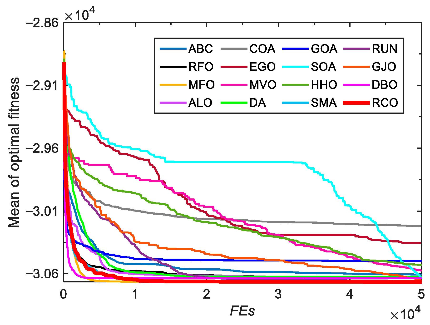
| RCO | −30,665.32349854 | 7.1895 × 10⁻¹ | −30,665.53867178 | −30,661.79892780 |
| DBO | −30,635.71460849 | 1.6335 × 10² | −30,665.53867178 | −29,770.81677325 |
| GJO | −30,657.37893505 | 4.1842 × 100 | −30,663.55315586 | −30,646.38130073 |
| RUN | −30,660.13539140 | 1.9969 × 101 | −30,665.53586489 | −30,561.69882047 |
| SMA | −30,665.53734918 | 1.5540 × 10⁻³ | −30,665.53865029 | −30,665.53262256 |
| HHO | −30,532.30441778 | 1.5263 × 10² | −30,663.48977472 | −30,201.43851773 |
| SOA | −30,641.70338442 | 1.7341 × 101 | −30,657.74185848 | −30,566.54192773 |
| GOA | −30,496.99193113 | 2.2198 × 10² | −30,665.43888010 | −29,837.56764245 |
| DA | −30,625.26683639 | 9.1543 × 101 | −30,665.53866631 | −30,342.54049981 |
| MVO | −30,575.23585370 | 7.9803 × 101 | −30,662.44936380 | −30,386.62854427 |
| EGO | −30,354.73643722 | 1.5849 × 10² | −30,634.70568304 | −30,085.99212698 |
| COA | −30,221.79295008 | 2.7718 × 10² | −30,660.04569407 | −29,657.05292693 |
| ALO | −30,624.67887473 | 1.0054 × 10² | −30,665.53858867 | −30,218.93339012 |
| MFO | −30,665.31055628 | 1.2452 × 100 | −30,665.53867178 | −30,658.71750920 |
| RFO | −30,658.81428956 | 1.8304 × 101 | −30,665.53867178 | −30,572.05049500 |
| ABC | −30,607.67379908 | 1.1696 × 101 | −30,630.43422662 | −30,584.93003770 |
Appendix B.2. I-Beam Design Problem

| Optimizer | Mean | Std | Best | Worst |
|---|---|---|---|---|
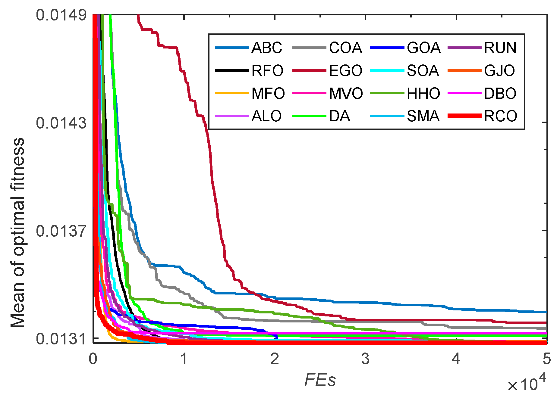
| RCO | 0.013074120217 | 7.0324 × 10⁻⁹ | 0.013074118905 | 0.013074157447 |
| DBO | 0.013129724700 | 2.1161 × 10⁻⁴ | 0.013074118905 | 0.013908205841 |
| GJO | 0.013074931995 | 6.2377 × 10⁻⁷ | 0.013074156740 | 0.013076087308 |
| RUN | 0.013074121447 | 2.4426 × 10⁻⁹ | 0.013074118987 | 0.013074128823 |
| SMA | 0.013074122152 | 1.3191 × 10⁻⁸ | 0.013074118913 | 0.013074191503 |
| HHO | 0.013075343023 | 5.1039 × 10⁻⁶ | 0.013074118905 | 0.013102198502 |
| SOA | 0.013076269212 | 2.0988 × 10⁻⁶ | 0.013074133499 | 0.013081247447 |
| GOA | 0.013074159564 | 2.1984 × 10⁻⁷ | 0.013074118905 | 0.013075323503 |
| DA | 0.013114850040 | 1.6511 × 10⁻⁴ | 0.013074118905 | 0.013908205863 |
| MVO | 0.013075030628 | 9.5513 × 10⁻⁷ | 0.013074134449 | 0.013078209725 |
| EGO | 0.013186062373 | 1.8456 × 10⁻⁴ | 0.013075003778 | 0.013818841015 |
| COA | 0.013156084492 | 2.3038 × 10⁻⁴ | 0.013074288457 | 0.013915045976 |
| ALO | 0.013080104310 | 1.7143 × 10⁻⁵ | 0.013074118913 | 0.013151854904 |
| MFO | 0.013083109110 | 4.8065 × 10⁻⁵ | 0.013074118905 | 0.013337561384 |
| RFO | 0.013074170655 | 8.5477 × 10⁻⁸ | 0.013074118905 | 0.013075136549 |
| ABC | 0.013247028789 | 3.3982 × 10⁻⁵ | 0.013139820756 | 0.013264707253 |
Appendix B.3. Tension/Compression Spring Design Problem
| Optimizer | Mean | Std | Best | Worst |
|---|---|---|---|---|
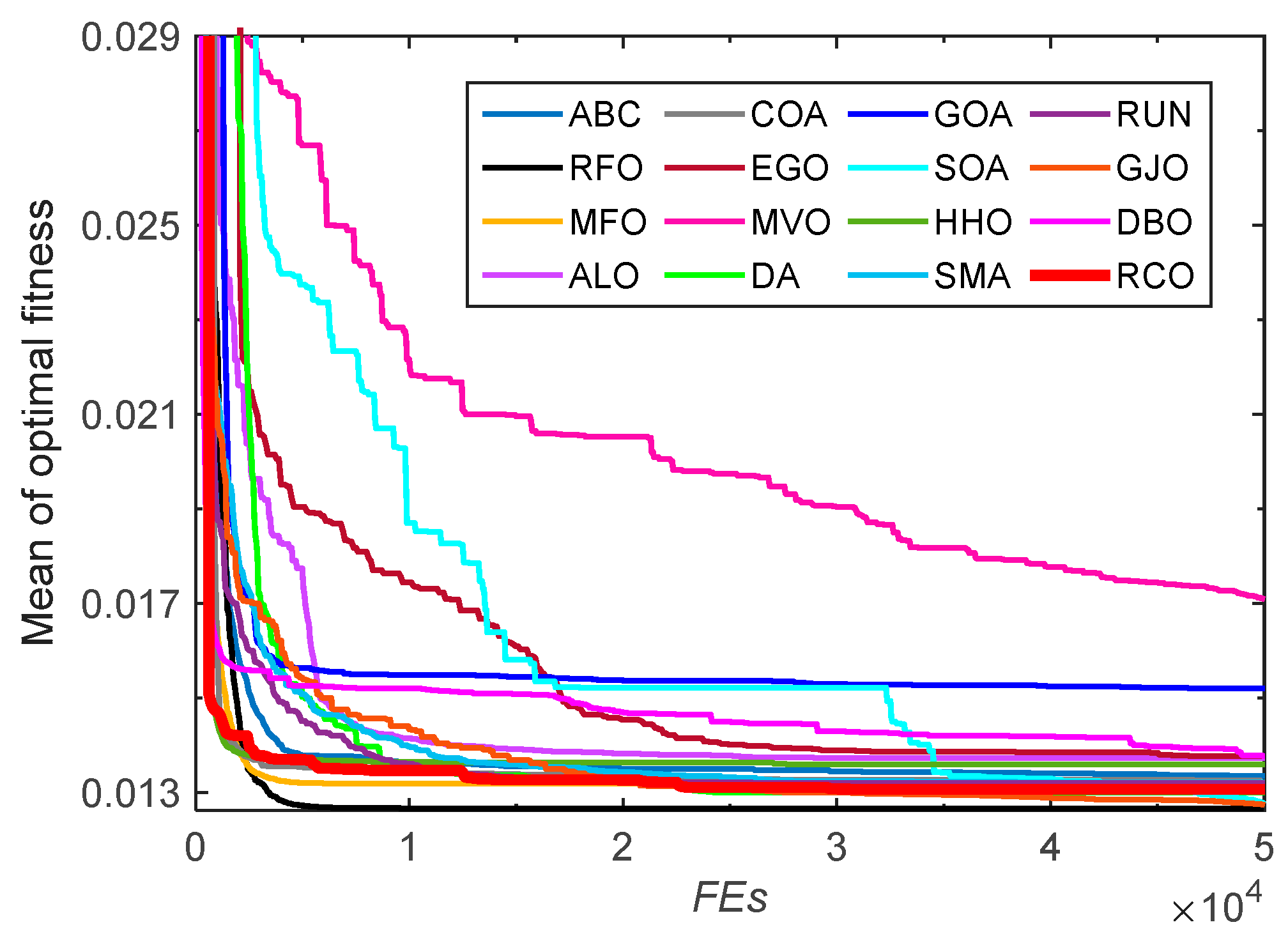
| RCO | 0.013053427666 | 7.8521 × 10⁻⁴ | 0.012665233831 | 0.015754390208 |
| DBO | 0.013772440263 | 1.8547 × 10⁻³ | 0.012665304859 | 0.017773158078 |
| GJO | 0.012736806942 | 4.4089 × 10⁻⁵ | 0.012684425803 | 0.012958545486 |
| RUN | 0.013197665660 | 1.0827 × 10⁻³ | 0.012666334447 | 0.017773164310 |
| SMA | 0.013213244427 | 7.3444 × 10⁻⁴ | 0.012669726461 | 0.015376704673 |
| HHO | 0.013597048937 | 9.5390 × 10⁻⁴ | 0.012666237221 | 0.017774812796 |
| SOA | 0.012752131110 | 2.2074 × 10⁻⁵ | 0.012704757407 | 0.012811498589 |
| GOA | 0.015198086272 | 1.9339 × 10⁻³ | 0.012668078008 | 0.017867196026 |
| DA | 0.012991820530 | 4.2921 × 10⁻⁴ | 0.012689820508 | 0.014901052692 |
| MVO | 0.017090902859 | 1.6960 × 10⁻³ | 0.012761974498 | 0.018383176280 |
| EGO | 0.013772491910 | 9.6876 × 10⁻⁴ | 0.012727047892 | 0.016798046250 |
| COA | 0.013258265593 | 8.7897 × 10⁻⁴ | 0.012685526191 | 0.017299772980 |
| ALO | 0.013724936736 | 1.5357 × 10⁻³ | 0.012672418461 | 0.017773186025 |
| MFO | 0.013188626844 | 1.0021 × 10⁻³ | 0.012667085044 | 0.017772992685 |
| RFO | 0.012665232789 | 5.6062 × 10⁻¹³ | 0.012665232788 | 0.012665232791 |
| ABC | 0.013349426786 | 2.4523 × 10⁻⁴ | 0.012865635902 | 0.013783878098 |
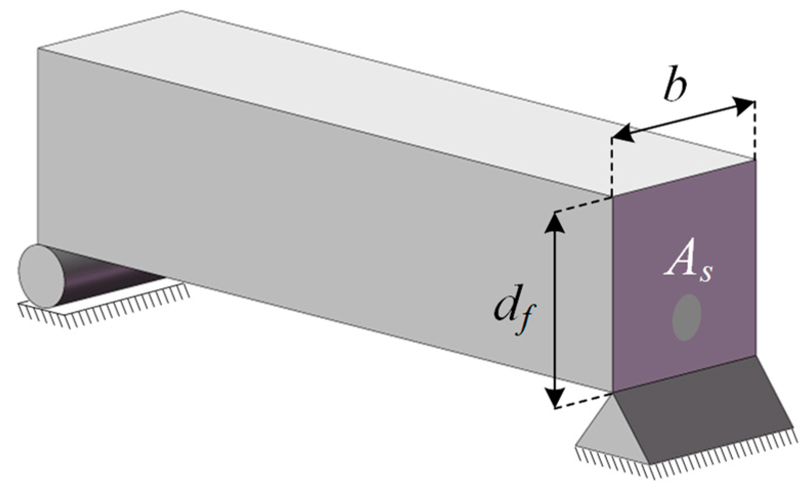
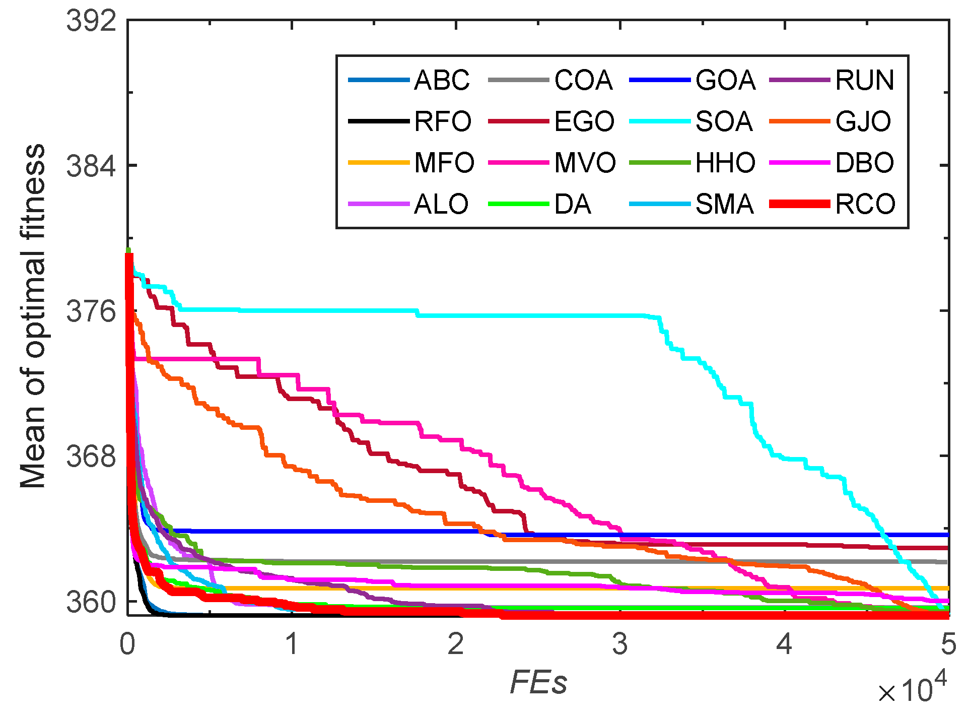
Appendix B.4. Reinforced Concrete Beam Design Problem
| Optimizer | Mean | Std | Best | Worst |
|---|---|---|---|---|
| RCO | 359.20799999 | 5.7815 × 10⁻¹⁴ | 359.20799999 | 359.20799999 |
| DBO | 360.01920035 | 1.3682 × 100 | 359.20799999 | 362.24999999 |
| GJO | 359.21173823 | 3.6435 × 10⁻³ | 359.20801045 | 359.22462089 |
| RUN | 359.30940274 | 5.5539 × 10⁻¹ | 359.20800001 | 362.25001392 |
| SMA | 359.32220003 | 6.2549 × 10⁻¹ | 359.20800000 | 362.63400001 |
| HHO | 359.43832098 | 8.6872 × 10⁻¹ | 359.20799999 | 362.63399999 |
| SOA | 359.23787686 | 2.6046 × 10⁻² | 359.20928087 | 359.29587381 |
| GOA | 363.64311954 | 5.2455 × 100 | 359.20799999 | 376.80000000 |
| DA | 359.61359999 | 1.0517 × 100 | 359.20799999 | 362.24999999 |
| MVO | 359.21213089 | 4.5808 × 10⁻³ | 359.20805144 | 359.22277961 |
| EGO | 362.92917939 | 1.6793 × 100 | 359.49427687 | 366.56462811 |
| COA | 362.16349552 | 2.9032 × 100 | 359.20800093 | 373.47135412 |
| ALO | 359.65200005 | 1.1529 × 100 | 359.20800000 | 362.63400012 |
| MFO | 360.70439999 | 1.6324 × 100 | 359.20799999 | 362.63399999 |
| RFO | 359.20799999 | 6.5919 × 10⁻¹⁴ | 359.20799999 | 359.20799999 |
| ABC | 359.20855745 | 9.3011 × 10⁻⁴ | 359.20800023 | 359.21200306 |
References
- Rao, S.S. Engineering Optimization: Theory and Practice, 4th ed.; John Wiley and Sons: Hoboken, NJ, USA, 1997. [Google Scholar]
- Houssein, E.H.; Elaziz, M.A.; Oliva, D.; Abualigah, L. Integrating Meta-Heuristics and Machine Learning for Real-World Optimization Problems; Springer Nature: Dordrecht, The Netherlands, 2022. [Google Scholar] [CrossRef]
- Wu, L.; Huang, X.; Cui, J.; Liu, C.; Xiao, W. Modified adaptive ant colony optimization algorithm and its application for solving path planning of mobile robot. Expert Syst. Appl. 2023, 215, 119410. [Google Scholar] [CrossRef]
- Dian, S.; Zhong, J.; Guo, B.; Liu, J.; Guo, R. A smooth path planning method for mobile robot using a BES-incorporated modified QPSO algorithm. Expert Syst. Appl. 2022, 208, 118256. [Google Scholar] [CrossRef]
- Zeng, W.; Zhu, W.; Hui, T.; Chen, L.; Xie, J.; Yu, T. An IMC-PID controller with particle swarm optimization algorithm for MSBR core power control. Nucl. Eng. Des. 2020, 360, 110513. [Google Scholar] [CrossRef]
- Qi, Z.; Shi, Q.; Zhang, H. Tuning of digital PID controllers using particle swarm optimization algorithm for a CAN-based DC motor subject to stochastic delays. IEEE Trans. Ind. Electron. 2020, 67, 5637–5646. [Google Scholar] [CrossRef]
- Kumari, M. 4—A review on metaheuristic algorithms: Recent and future trends. In Metaheuristics-Based Materials Optimization; Elsevier: Amsterdam, The Netherlands, 2025; pp. 103–128. [Google Scholar] [CrossRef]
- Rajwar, K.; Deep, K.; Das, S. An exhaustive review of the metaheuristic algorithms for search and optimization: Taxonomy, applications, and open challenges. Artif. Intell. Rev. 2023, 56, 13187–13257. [Google Scholar] [CrossRef]
- Holland, J.H. Genetic algorithms. Sci. Am. 1992, 267, 66–73. [Google Scholar] [CrossRef]
- Storn, R.; Price, K. Differential evolution—A simple and efficient heuristic for global optimization over continuous spaces. J. Glob. Optim. 1997, 11, 341–359. [Google Scholar] [CrossRef]
- Kennedy, J.; Eberhart, R. Particle swarm optimization. In Proceedings of the ICNN’95—International Conference on Neural Networks, Perth, Australia, 27 November–1 December 1995; pp. 1942–1948. [Google Scholar] [CrossRef]
- Karaboga, D.; Basturk, B. Artificial bee colony (ABC) optimization algorithm for solving constrained optimization problems. In Proceedings of the 12th International Fuzzy Systems Association World Congress, Cancun, Mexico, 18–21 June 2007; pp. 789–798. [Google Scholar] [CrossRef]
- Pan, W. A new fruit fly optimization algorithm: Taking the financial distress model as an example. Knowl.-Based Syst. 2012, 26, 69–74. [Google Scholar] [CrossRef]
- Mirjalili, S.; Mirjalili, S.M.; Lewis, A. Grey wolf optimizer. Adv. Eng. Softw. 2014, 69, 46–61. [Google Scholar] [CrossRef]
- Arora, S.; Singh, S. Butterfly algorithm with Lèvy flights for global optimization. In Proceedings of the 2015 International Conference on Signal Processing, Computing and Control, Solan, India, 24–26 September 2015; pp. 220–224. [Google Scholar] [CrossRef]
- Mirjalili, S.; Lewis, A. The whale optimization algorithm. Adv. Eng. Softw. 2016, 95, 51–67. [Google Scholar] [CrossRef]
- Mirjalili, S. Dragonfly algorithm: A new meta-heuristic optimization technique for solving single-objective, discrete, and multi-objective problems. Neural Comput. Appl. 2016, 27, 1053–1073. [Google Scholar] [CrossRef]
- Rao, R.V.; Savsani, V.J.; Vakharia, D.P. Teaching-learning-based optimization: A novel method for constrained mechanical design optimization problems. Comput.-Aided Des. 2011, 43, 303–315. [Google Scholar] [CrossRef]
- Das, B.; Mukherjee, V.; Das, D. Student psychology based optimization algorithm: A new population based optimization algorithm for solving optimization problems. Adv. Eng. Softw. 2020, 146, 102804. [Google Scholar] [CrossRef]
- Feng, Z.; Niu, W.; Liu, S. Cooperation search algorithm: A novel metaheuristic evolutionary intelligence algorithm for numerical optimization and engineering optimization problems. Appl. Soft Comput. 2021, 98, 106734. [Google Scholar] [CrossRef]
- Trojovská, E.; Dehghani, M. A new human-based metahurestic optimization method based on mimicking cooking training. Sci. Rep. 2022, 12, 14861. [Google Scholar] [CrossRef] [PubMed]
- Dehghani, M.; Trojovská, E.; Trojovský, P. A new human-based metaheuristic algorithm for solving optimization problems on the base of simulation of driving training process. Sci. Rep. 2022, 12, 9924. [Google Scholar] [CrossRef]
- Rashedi, E.; Nezamabadi-pour, H.; Saryazdi, S. GSA: A gravitational search algorithm. Inf. Sci. 2009, 179, 2232–2248. [Google Scholar] [CrossRef]
- Mirjalili, S.; Mirjalili, S.M.; Hatamlou, A. Multi-verse optimizer: A nature-inspired algorithm for global optimization. Neural Comput. Appl. 2016, 27, 495–513. [Google Scholar] [CrossRef]
- Talatahari, S.; Azizi, M.; Gandomi, A.H. Material generation algorithm: A novel metaheuristic algorithm for optimization of engineering problems. Processes 2021, 9, 859. [Google Scholar] [CrossRef]
- Hashim, F.A.; Mostafa, R.R.; Hussien, A.G.; Mirjalili, S.; Sallam, K.M. Fick’s law algorithm: A physical law-based algorithm for numerical optimization. Knowl.-Based Syst. 2023, 260, 110146. [Google Scholar] [CrossRef]
- Mirjalili, S. SCA: A sine cosine algorithm for solving optimization problems. Knowl.-Based Syst. 2016, 96, 120–133. [Google Scholar] [CrossRef]
- Abualigah, L.; Diabat, A.; Mirjalili, S.; Elaziz, M.A.; Gandomi, A.H. The arithmetic optimization algorithm. Comput. Methods Appl. Mech. Eng. 2021, 376, 113609. [Google Scholar] [CrossRef]
- Yang, Y.; Chen, H.; Heidari, A.A.; Gandomi, A.H. Hunger games search: Visions, conception, implementation, deep analysis, perspectives, and towards performance shifts. Expert Syst. Appl. 2021, 177, 114864. [Google Scholar] [CrossRef]
- Dehghani, M.; Mardaneh, M.; Guerrero, J.M.; Malik, O.P.; Kumar, V. Football game based optimization: An application to solve energy commitment problem. Int. J. Intell. Eng. Syst. 2020, 13, 514–523. [Google Scholar] [CrossRef]
- Koza, J.R. Genetic Programming: On the Programming of Computers by Means of Natural Selection; MIT Press: Cambridge, MA, USA, 1992. [Google Scholar]
- Mirjalili, S. Moth-flame optimization algorithm: A novel nature-inspired heuristic paradigm. Knowl.-Based Syst. 2015, 89, 228–249. [Google Scholar] [CrossRef]
- Heidari, A.A.; Mirjalili, S.; Faris, H.; Aljarah, I.; Mafarja, M.; Chen, H. Harris hawks optimization: Algorithm and applications. Future Gener. Comput. Syst. 2019, 97, 849–872. [Google Scholar] [CrossRef]
- Xue, J.; Shen, B. Dung beetle optimizer: A new meta-heuristic algorithm for global optimization. J. Supercomput. 2023, 79, 7305–7336. [Google Scholar] [CrossRef]
- Abdel-Basset, M.; Mohamed, R.; Zidan, M.; Jameel, M.; Abouhawwash, M. Mantis search algorithm: A novel bio-inspired algorithm for global optimization and engineering design problems. Comput. Methods Appl. Mech. Eng. 2023, 415, 116200. [Google Scholar] [CrossRef]
- Talatahari, S.; Bayzidi, H.; Saraee, M. Social network search for global optimization. IEEE Access 2021, 9, 92815–92863. [Google Scholar] [CrossRef]
- Kirkpatrick, S.; Gelatt, C.D.; Vecchi, M.P. Optimization by simulated annealing. Science 1983, 220, 671–680. [Google Scholar] [CrossRef]
- Ahmadianfar, I.; Heidari, A.A.; Noshadian, S.; Chen, H.; Gandomi, A.H. INFO: An efficient optimization algorithm based on weighted mean of vectors. Expert Syst. Appl. 2022, 195, 116516. [Google Scholar] [CrossRef]
- Lynn, N.; Suganthan, P.N. Heterogeneous comprehensive learning particle swarm optimization with enhanced exploration and exploitation. Swarm Evol. Comput. 2015, 24, 11–24. [Google Scholar] [CrossRef]
- Han, B.; Li, B.; Qin, C. A novel hybrid particle swarm optimization with marine predators. Swarm Evol. Comput. 2023, 83, 101375. [Google Scholar] [CrossRef]
- Chopra, N.; Ansari, M.M. Golden jackal optimization: A novel nature-inspired optimizer for engineering applications. Expert Syst. Appl. 2022, 198, 116924. [Google Scholar] [CrossRef]
- Li, S.; Chen, H.; Wang, M.; Heidari, A.A.; Mirjalili, S. Slime mould algorithm: A new method for stochastic optimization. Future Gener. Comput. Syst. 2020, 111, 300–323. [Google Scholar] [CrossRef]
- Inoue, M.; Shimura, R.; Uebayashi, A.; Ikoma, S.; Iima, H.; Sumiyoshi, T.; Teraoka, H.; Makita, K.; Hiraga, T.; Momose, K.; et al. Physical body parameters of red-crowned cranes Grus japonensis by sex and life stage in eastern Hokkaido, Japan. J. Vet. Med. Sci. 2013, 75, 1055–1060. [Google Scholar] [CrossRef] [PubMed]
- Wikipedia Contributors. Red-Crowned Crane. Wikipedia, The Free Encyclopedia. Available online: https://en.wikipedia.org/w/index.php?title=Red-crowned_crane&oldid=1180027726 (accessed on 15 May 2025).
- Su, L.; Zou, H. Status, threats and conservation needs for the continental population of the red-crowned crane. Chin. Birds 2012, 3, 147–164. [Google Scholar] [CrossRef]
- Xu, P.; Zhang, X.; Zhang, F.; Bempah, G.; Lu, C.; Lv, S.; Zhang, W.; Cui, P. Use of aquaculture ponds by globally endangered red-crowned crane (Grus japonensis) during the wintering period in the Yancheng National Nature Reserve, a Ramsar wetland. Glob. Ecol. Conserv. 2020, 23, e01123. [Google Scholar] [CrossRef]
- Liu, L.; Liao, J.; Wu, Y.; Zhang, Y. Breeding range shift of the red-crowned crane (Grus japonensis) under climate change. PLoS ONE 2020, 15, e0229984. [Google Scholar] [CrossRef]
- Takeda, K.F.; Kutsukake, N. Complexity of mutual communication in animals exemplified by paired dances in the red-crowned crane. Jpn. J. Anim. Psychol. 2018, 68, 25–37. [Google Scholar] [CrossRef]
- Nenavath, H.; Jatoth, R.K.; Das, S. A synergy of the sine-cosine algorithm and particle swarm optimizer for improved global optimization and object tracking. Swarm Evol. Comput. 2018, 43, 1–30. [Google Scholar] [CrossRef]
- Su, H.; Zhao, D.; Heidari, A.A.; Liu, L.; Zhang, X.; Mafarja, M.; Chen, H. RIME: A physics-based optimization. Neurocomputing 2023, 532, 183–214. [Google Scholar] [CrossRef]
- Braik, M.; Al-Hiary, H. Rüppell’s fox optimizer: A novel meta-heuristic approach for solving global optimization problems. Clust. Comput. 2025, 28, 292. [Google Scholar] [CrossRef]
- Mohammadzadeh, A.; Mirjalili, S. Eel and grouper optimizer: A nature-inspired optimization algorithm. Clust. Comput. 2024, 27, 12745–12786. [Google Scholar] [CrossRef]
- Dehghani, M.; Montazeri, Z.; Trojovská, E.; Trojovský, P. Coati optimization algorithm: A new bio-inspired metaheuristic algorithm for solving optimization problems. Knowl.-Based Syst. 2023, 259, 110011. [Google Scholar] [CrossRef]
- Ahmadianfar, I.; Heidari, A.A.; Gandomi, A.H.; Chu, X.; Chen, H. RUN beyond the metaphor: An efficient optimization algorithm based on Runge Kutta method. Expert Syst. Appl. 2021, 181, 115079. [Google Scholar] [CrossRef]
- Mirjalili, S. The ant lion optimizer. Adv. Eng. Softw. 2015, 83, 80–98. [Google Scholar] [CrossRef]
- Saremi, S.; Mirjalili, S.; Lewis, A. Grasshopper optimisation algorithm: Theory and application. Adv. Eng. Softw. 2017, 105, 30–47. [Google Scholar] [CrossRef]
- Dhiman, G.; Kumar, V. Seagull optimization algorithm: Theory and its applications for large-scale industrial engineering problems. Knowl.-Based Syst. 2019, 165, 169–196. [Google Scholar] [CrossRef]
- Ray, T.; Saini, P. Engineering design optimization using a swarm with an intelligent information sharing among individuals. Eng. Optim. 2001, 33, 735–748. [Google Scholar] [CrossRef]
- Chickermane, H.; Gea, H.C. Structural optimization using a new local approximation method. Int. J. Numer. Methods Eng. 1996, 39, 829–846. [Google Scholar] [CrossRef]
- Ravindran, A.; Ragsdell, K.M.; Reklaitis, G.V. Engineering Optimization: Methods and Applications; Wiley: Hoboken, NJ, USA, 2006. [Google Scholar]
- Akhtar, S.; Tai, K.; Ray, T. A socio-behavioural simulation model for engineering design optimization. Eng. Optim. 2002, 34, 341–354. [Google Scholar] [CrossRef]
- Zavala, A.E.M.; Aguirre, A.H.; Diharce, E.R.V. Particle evolutionary swarm optimization with linearly decreasing ε-tolerance. In Proceedings of the MICAI 2005: Advances in Artificial Intelligence, Monterrey, Mexico, 14–18 November 2005; pp. 641–651. [Google Scholar] [CrossRef]
- Osyczka, A. Multicriteria optimization for engineering design. In Design Optimization; Academic Press: Cambridge, MA, USA, 1985; pp. 193–227. [Google Scholar] [CrossRef]
- Coello, C.A.C. Use of a self-adaptive penalty approach for engineering optimization problems. Comput. Ind. 2000, 41, 113–127. [Google Scholar] [CrossRef]
- Amir, H.M.; Hasegawa, T. Nonlinear mixed-discrete structural optimization. J. Struct. Eng. 1989, 115, 626–646. [Google Scholar] [CrossRef]
- Coello, C.A.C. Theoretical and numerical constraint-handling techniques used with evolutionary algorithms: A survey of the state of the art. Comput. Methods Appl. Mech. Eng. 2002, 191, 1245–1287. [Google Scholar] [CrossRef]

| Type | Algorithm | Inspiration |
|---|---|---|
| Evolution-based | Genetic Algorithm (GA) [9] | Mutation, crossover, and natural selection strategies |
| Genetic Programming (GP) [31] | Inherited the basic idea of GA | |
| Differential Evolution (DE) [10] | Inherited the basic idea of GA | |
| Swarm-based | Particle Swarm Optimization (PSO) [11] | Predation behavior of birds |
| Grey Wolf Optimizer (GWO) [14] | Hierarchy and hunting behavior of gray wolves | |
| Moth–Flame Optimization (MFO) [32] | Navigation method of moths | |
| Harris Hawks Optimizer (HHO) [33] | Cooperative and chasing behaviors of Harris’ hawks | |
| Dung Beetle Optimizer (DBO) [34] | Five behaviors of dung beetles | |
| Mantis Search Algorithm (MSA) [35] | Hunting and sexual cannibalism of praying mantises | |
| Human-based | Teaching–Learning-Based Optimization (TLBO) [18] | Impact of teachers on student learning |
| Student Psychology-Based Optimization (SPBO) [19] | Psychology of students expecting for progress | |
| Social Network Search (SNS) [36] | Interactive behavior among users in social networks | |
| Physics- and chemistry-based | Simulated Annealing (SA) [37] | Annealing process in physics |
| Gravitational Search Algorithm (GSA) [23] | Newton’s law of universal gravitation | |
| Multi-Verse Optimizer (MVO) [24] | Concepts of white hole, black hole, and wormhole | |
| Others | Sine–Cosine Algorithm (SCA) [27] | Mathematical model of sine and cosine functions |
| Arithmetic Optimization Algorithm (AOA) [28] | Main arithmetic operators in mathematics | |
| Weighted Mean of Vectors (INFO) [38] | Idea of weighted mean |
| Algorithm | Parameter Settings |
|---|---|
| RCO | pc = 0.7, k:(n − k) = 1:1 |
| DBO | k = λ = 0.1, b = 0.3, S = 0.5 |
| GJO | c1 = 1.5 |
| RUN | a = 20, b = 12 |
| SMA | vc = 1 − t/tmax, z = 0.03 |
| HHO | E0 randomly changes in (−1,1) |
| COA | I randomly changes in {1,2} |
| EGO | a = 2 − 2*t/tmax |
| RFO | β = 0.000001, e0 = 1, e1 = 3, c0 = 2, c1 = 2, a0 = 2, a1 = 3 |
| Index | RCO vs. DBO | RCO vs. GJO | RCO vs. RUN | RCO vs. SMA | RCO vs. HHO | RCO vs. COA | RCO vs. EGO | RCO vs. RFO | |
|---|---|---|---|---|---|---|---|---|---|
| F1 | p-value | 2.5631 × 10⁻⁶ | 1.7344 × 10⁻⁶ | 1.7344 × 10⁻⁶ | 1 | 1.7344 × 10⁻⁶ | 1.7344 × 10⁻⁶ | 1 | 1.7344 × 10⁻⁶ |
| R+ | 0 | 0 | 0 | 0 | 0 | 0 | 0 | 0 | |
| R− | 435 | 465 | 465 | 0 | 465 | 465 | 0 | 465 | |
| +/=/− | + | + | + | = | + | + | = | + | |
| F2 | p-value | 1.7344 × 10⁻⁶ | 1.7344 × 10⁻⁶ | 1.7344 × 10⁻⁶ | 2.1336 × 10⁻¹ | 1.7344 × 10⁻⁶ | 1.7344 × 10⁻⁶ | 1.7344 × 10⁻⁶ | 1.7344 × 10⁻⁶ |
| R+ | 0 | 0 | 0 | 172 | 0 | 0 | 0 | 0 | |
| R− | 465 | 465 | 465 | 293 | 465 | 465 | 465 | 465 | |
| +/=/− | + | + | + | = | + | + | + | + | |
| F3 | p-value | 1.7344 × 10⁻⁶ | 1.7344 × 10⁻⁶ | 1.7344 × 10⁻⁶ | 1 | 1.7344 × 10⁻⁶ | 1.7344 × 10⁻⁶ | 1 | 1.7344 × 10⁻⁶ |
| R+ | 0 | 0 | 0 | 0 | 0 | 0 | 0 | 0 | |
| R− | 465 | 465 | 465 | 0 | 465 | 465 | 0 | 465 | |
| +/=/− | + | + | + | = | + | + | = | + | |
| F4 | p-value | 1.7344 × 10⁻⁶ | 1.7344 × 10⁻⁶ | 1.7344 × 10⁻⁶ | 1.2544 × 10⁻¹ | 1.7344 × 10⁻⁶ | 1.7344 × 10⁻⁶ | 1.7344 × 10⁻⁶ | 1.7344 × 10⁻⁶ |
| R+ | 0 | 0 | 0 | 307 | 0 | 0 | 0 | 0 | |
| R− | 465 | 465 | 465 | 158 | 465 | 465 | 465 | 465 | |
| +/=/− | + | + | + | = | + | + | + | + | |
| F5 | p-value | 1.7344 × 10⁻⁶ | 1.7344 × 10⁻⁶ | 3.1849 × 10⁻¹ | 1.7344 × 10⁻⁶ | 1.7344 × 10⁻⁶ | 1.7344 × 10⁻⁶ | 1.7344 × 10⁻⁶ | 1.9209 × 10⁻⁶ |
| R+ | 0 | 0 | 281 | 465 | 465 | 465 | 0 | 464 | |
| R− | 465 | 465 | 184 | 0 | 0 | 0 | 465 | 1 | |
| +/=/− | + | + | = | − | − | − | + | − | |
| F6 | p-value | 1.7344 × 10⁻⁶ | 1.7344 × 10⁻⁶ | 1.7344 × 10⁻⁶ | 1.7344 × 10⁻⁶ | 3.8822 × 10⁻⁶ | 1.7344 × 10⁻⁶ | 1.7344 × 10⁻⁶ | 1.7344 × 10⁻⁶ |
| R+ | 465 | 0 | 465 | 0 | 8 | 0 | 0 | 0 | |
| R− | 0 | 465 | 0 | 465 | 457 | 465 | 465 | 465 | |
| +/=/− | − | + | − | + | + | + | + | + | |
| F7 | p-value | 1.7344 × 10⁻⁶ | 1.9646 × 10⁻³ | 1.3601 × 10⁻⁵ | 1.8326 × 10⁻³ | 2.2102 × 10⁻¹ | 5.8571 × 10⁻¹ | 3.2857 × 10⁻¹ | 1.7344 × 10⁻⁶ |
| R+ | 0 | 82 | 21 | 81 | 173 | 259 | 280 | 0 | |
| R− | 465 | 383 | 444 | 384 | 292 | 206 | 185 | 465 | |
| +/=/− | + | + | + | + | = | = | = | + | |
| F8 | p-value | 1.7988 × 10⁻⁵ | 1.7344 × 10⁻⁶ | 9.2710 × 10⁻³ | 1.7344 × 10⁻⁶ | 1.7344 × 10⁻⁶ | 1.7344 × 10⁻⁶ | 8.9443 × 10⁻⁴ | 4.4463 × 10⁻² |
| R+ | 441 | 0 | 359 | 465 | 465 | 465 | 71 | 139 | |
| R− | 24 | 465 | 106 | 0 | 0 | 0 | 394 | 326 | |
| +/=/− | − | + | − | − | − | − | + | + | |
| F9 | p-value | 1 | 1 | 1 | 1 | 1 | 1 | 1 | 3.1250 × 10⁻² |
| R+ | 0 | 0 | 0 | 0 | 0 | 0 | 0 | 0 | |
| R− | 0 | 0 | 0 | 0 | 0 | 0 | 0 | 21 | |
| +/=/− | = | = | = | = | = | = | = | + | |
| F10 | p-value | 1 | 1.0135 × 10⁻⁷ | 1 | 1 | 1 | 1 | 1 | 1 |
| R+ | 0 | 0 | 0 | 0 | 0 | 0 | 0 | 0 | |
| R− | 0 | 465 | 0 | 0 | 0 | 0 | 0 | 0 | |
| +/=/− | = | + | = | = | = | = | = | = | |
| F11 | p-value | 1 | 1 | 1 | 1 | 1 | 1 | 1 | 1.2500 × 10⁻¹ |
| R+ | 0 | 0 | 0 | 0 | 0 | 0 | 0 | 0 | |
| R− | 0 | 0 | 0 | 0 | 0 | 0 | 0 | 10 | |
| +/=/− | = | = | = | = | = | = | = | = | |
| F12 | p-value | 3.1123 × 10⁻⁵ | 1.7344 × 10⁻⁶ | 1.7344 × 10⁻⁶ | 1.7344 × 10⁻⁶ | 2.7653 × 10⁻³ | 1.7344 × 10⁻⁶ | 1.7344 × 10⁻⁶ | 1.2544 × 10⁻¹ |
| R+ | 435 | 0 | 465 | 0 | 87 | 0 | 0 | 158 | |
| R− | 30 | 465 | 0 | 465 | 378 | 465 | 465 | 307 | |
| +/=/− | − | + | − | + | + | + | + | = | |
| F13 | p-value | 4.2857 × 10⁻⁶ | 1.7088 × 10⁻³ | 2.1266 × 10⁻⁶ | 1.9209 × 10⁻⁶ | 1.7344 × 10⁻⁶ | 1.7344 × 10⁻⁶ | 6.7328 × 10⁻¹ | 1.7344 × 10⁻⁶ |
| R+ | 456 | 80 | 463 | 464 | 465 | 465 | 253 | 465 | |
| R− | 9 | 385 | 2 | 1 | 0 | 0 | 212 | 0 | |
| +/=/− | − | + | − | − | − | − | = | − | |
| F14 | p-value | 1.0881 × 10⁻¹ | 1.6678 × 10⁻⁶ | 4.7045 × 10⁻⁴ | 2.4730 × 10⁻⁶ | 2.5631 × 10⁻⁶ | 5.6061 × 10⁻⁶ | 1.7344 × 10⁻⁶ | 1 |
| R+ | 0 | 0 | 0 | 0 | 0 | 0 | 0 | 0 | |
| R− | 6 | 465 | 120 | 435 | 435 | 378 | 465 | 0 | |
| +/=/− | = | + | + | + | + | + | + | = | |
| F15 | p-value | 2.0515 × 10⁻⁴ | 1.1093 × 10⁻¹ | 1.9569 × 10⁻² | 1.8326 × 10⁻³ | 4.9498 × 10⁻² | 1.3601 × 10⁻⁵ | 4.1955 × 10⁻⁴ | 6.7328 × 10⁻¹ |
| R+ | 52 | 310 | 119 | 81 | 137 | 21 | 61 | 253 | |
| R− | 413 | 155 | 346 | 384 | 328 | 444 | 404 | 212 | |
| +/=/− | + | = | + | + | + | + | + | = | |
| F16 | p-value | 1 | 1.7344 × 10⁻⁶ | 3.8710 × 10⁻⁵ | 1.7279 × 10⁻⁶ | 7.6227 × 10⁻⁴ | 2.5631 × 10⁻⁶ | 1.7344 × 10⁻⁶ | 1 |
| R+ | 0 | 0 | 0 | 0 | 0 | 0 | 0 | 0 | |
| R− | 0 | 465 | 253 | 465 | 105 | 435 | 465 | 0 | |
| +/=/− | = | + | + | + | + | + | + | = | |
| F17 | p-value | 1 | 1.7344 × 10⁻⁶ | 2.6414 × 10⁻⁵ | 1.7344 × 10⁻⁶ | 8.2981 × 10⁻⁶ | 1.7344 × 10⁻⁶ | 1.7344 × 10⁻⁶ | 1 |
| R+ | 0 | 0 | 0 | 0 | 0 | 0 | 0 | 0 | |
| R− | 0 | 465 | 276 | 465 | 351 | 465 | 465 | 0 | |
| +/=/− | = | + | + | + | + | + | + | = | |
| F18 | p-value | 2.8557 × 10⁻⁵ | 1.7344 × 10⁻⁶ | 1.8072 × 10⁻⁵ | 1.7257 × 10⁻⁶ | 2.5596 × 10⁻⁶ | 1.7344 × 10⁻⁶ | 1.7344 × 10⁻⁶ | 1 |
| R+ | 0 | 0 | 0 | 0 | 0 | 0 | 0 | 0 | |
| R− | 190 | 465 | 300 | 465 | 435 | 465 | 465 | 0 | |
| +/=/− | + | + | + | + | + | + | + | = | |
| F19 | p-value | 4.0479 × 10⁻² | 1.7344 × 10⁻⁶ | 1.7344 × 10⁻⁶ | 1.7344 × 10⁻⁶ | 1.7344 × 10⁻⁶ | 1.7344 × 10⁻⁶ | 1.7344 × 10⁻⁶ | 1 |
| R+ | 1 | 0 | 0 | 0 | 0 | 0 | 0 | 0 | |
| R− | 20 | 465 | 465 | 465 | 465 | 465 | 465 | 0 | |
| +/=/− | + | + | + | + | + | + | + | = | |
| F20 | p-value | 3.2082 × 10⁻² | 3.1123 × 10⁻⁵ | 2.1053 × 10⁻³ | 1.3601 × 10⁻⁵ | 1.6046 × 10⁻⁴ | 1.7344 × 10⁻⁶ | 4.0702 × 10⁻² | 7.2488 × 10⁻¹ |
| R+ | 36.5 | 30 | 83 | 21 | 49 | 0 | 133 | 149.5 | |
| R− | 134.5 | 435 | 382 | 444 | 416 | 465 | 332 | 175.5 | |
| +/=/− | + | + | + | + | + | + | + | = | |
| F21 | p-value | 1.8965 × 10⁻⁴ | 1.7344 × 10⁻⁶ | 1.7344 × 10⁻⁶ | 1.7344 × 10⁻⁶ | 1.7344 × 10⁻⁶ | 1.7344 × 10⁻⁶ | 1.7344 × 10⁻⁶ | 9.7656 × 10⁻⁴ |
| R+ | 0 | 0 | 0 | 0 | 0 | 0 | 0 | 0 | |
| R− | 171 | 465 | 465 | 465 | 465 | 465 | 465 | 66 | |
| +/=/− | + | + | + | + | + | + | + | + | |
| F22 | p-value | 6.2096 × 10⁻⁴ | 1.7344 × 10⁻⁶ | 1.7344 × 10⁻⁶ | 1.7344 × 10⁻⁶ | 1.7344 × 10⁻⁶ | 1.7344 × 10⁻⁶ | 1.7344 × 10⁻⁶ | 1.5625 × 10⁻² |
| R+ | 0 | 0 | 0 | 0 | 0 | 0 | 0 | 0 | |
| R− | 120 | 465 | 465 | 465 | 465 | 465 | 465 | 28 | |
| +/=/− | + | + | + | + | + | + | + | + | |
| F23 | p-value | 3.1915 × 10⁻³ | 1.7344 × 10⁻⁶ | 1.7344 × 10⁻⁶ | 1.7344 × 10⁻⁶ | 1.7344 × 10⁻⁶ | 1.7344 × 10⁻⁶ | 1.7344 × 10⁻⁶ | 1.9531 × 10⁻³ |
| R+ | 0 | 0 | 0 | 0 | 0 | 0 | 0 | 0 | |
| R− | 66 | 465 | 465 | 465 | 465 | 465 | 465 | 55 | |
| +/=/− | + | + | + | + | + | + | + | + | |
| Unimodal (+/=/−) | 6/0/1 | 7/0/0 | 5/1/1 | 2/4/1 | 5/1/1 | 5/1/1 | 4/3/0 | 6/0/1 | |
| Multimodal (+/=/−) | 7/6/3 | 13/3/0 | 10/3/3 | 11/3/2 | 11/3/2 | 11/3/2 | 12/4/0 | 5/10/1 | |
| Total (+/=/−) | 13/6/4 | 20/3/0 | 15/4/4 | 13/7/3 | 16/4/3 | 16/4/3 | 16/7/0 | 11/10/2 | |
| Index | RCO | DBO | GJO | RUN | SMA | HHO | COA | EGO | RFO | |
|---|---|---|---|---|---|---|---|---|---|---|
| F1 | Mean | 0 | 3.2549 × 10−234 | 4.9056 × 10⁻³⁴ | 5.1469 × 10−206 | 0 | 1.0271 × 10−187 | 1.0905 × 10−300 | 0 | 1.2147 × 10−116 |
| Std | 0 | 1.7826 × 10−233 | 5.4342 × 10⁻³⁴ | 2.8173 × 10−205 | 0 | 5.6213 × 10−187 | 5.9725 × 10−300 | 0 | 6.6469 × 10−116 | |
| Min | 0 | 3.7701 × 10−297 | 3.1716 × 10⁻³⁵ | 2.6183 × 10−229 | 0 | 3.0699 × 10−213 | 0 | 0 | 3.8455 × 10−146 | |
| Max | 0 | 9.7636 × 10−233 | 2.1880 × 10⁻³³ | 1.5431 × 10−204 | 0 | 3.0790 × 10−186 | 3.2713 × 10−299 | 0 | 3.6408 × 10−115 | |
| Rank | 1 | 5 | 9 | 6 | 1 | 7 | 4 | 1 | 8 | |
| F2 | Mean | 1.6764 × 10−231 | 8.2119 × 10−125 | 1.1235 × 10⁻²¹ | 3.2985 × 10−117 | 1.2861 × 10⁻¹ | 2.8828 × 10−99 | 1.2626 × 10−151 | 9.3039 × 10−224 | 1.9514 × 10−60 |
| Std | 9.0402 × 10−231 | 3.6042 × 10−124 | 7.4570 × 10⁻²² | 1.7917 × 10−116 | 4.5867 × 10⁻¹ | 9.0091 × 10−99 | 5.6229 × 10−151 | 5.0513 × 10−223 | 1.0687 × 10−59 | |
| Min | 1.8057 × 10−269 | 1.9735 × 10−151 | 3.3215 × 10⁻²² | 2.9994 × 10−126 | 3.2039 × 10−62 | 9.6944 × 10−110 | 4.0545 × 10−163 | 1.0810 × 10−233 | 2.0457 × 10−76 | |
| Max | 4.9536 × 10−230 | 1.9349 × 10−123 | 4.4806 × 10⁻²¹ | 9.8163 × 10−116 | 2.3614 × 100 | 4.0818 × 10−98 | 3.0789 × 10−150 | 2.7674 × 10−222 | 5.8533 × 10−59 | |
| Rank | 1 | 4 | 8 | 5 | 9 | 6 | 3 | 2 | 7 | |
| F3 | Mean | 0 | 5.5813 × 10−59 | 1.3174 × 10³ | 8.8613 × 10−170 | 2.9198 × 10−204 | 2.2178 × 10−99 | 1.7681 × 10−300 | 0 | 3.5998 × 10⁻³³ |
| Std | 0 | 3.0570 × 10−59 | 3.9531 × 10³ | 4.8535 × 10−169 | 1.5993 × 10−203 | 1.2147 × 10−98 | 9.6727 × 10−300 | 0 | 1.7931 × 10⁻³² | |
| Min | 0 | 8.8207 × 10−256 | 2.6831 × 10⁻² | 7.1550 × 10−194 | 0 | 1.7423 × 10−163 | 8.0533 × 10−322 | 0 | 7.6499 × 10−62 | |
| Max | 0 | 1.6744 × 10−58 | 1.9815 × 10⁴ | 2.6584 × 10−168 | 8.7595 × 10−203 | 6.6534 × 10−98 | 5.2982 × 10−299 | 0 | 9.8324 × 10⁻³² | |
| Rank | 1 | 7 | 9 | 5 | 4 | 6 | 3 | 1 | 8 | |
| F4 | Mean | 1.2991 × 10−221 | 3.1022 × 10−86 | 7.3632 × 101 | 4.0938 × 10−98 | 1.7504 × 10−151 | 8.2143 × 10−96 | 3.9586 × 10−153 | 9.9172 × 10−197 | 1.1167 × 10⁻³² |
| Std | 7.1135 × 10−221 | 1.3699 × 10−85 | 5.4243 × 100 | 1.8918 × 10−97 | 9.5872 × 10−151 | 3.3751 × 10−95 | 1.1159 × 10−152 | 3.7978 × 10−196 | 3.5729 × 10⁻³² | |
| Min | 1.1104 × 10−263 | 6.2548 × 10−145 | 6.3334 × 101 | 1.5590 × 10−111 | 0 | 3.1642 × 10−107 | 1.0136 × 10−161 | 7.2829 × 10−204 | 1.1963 × 10−43 | |
| Max | 3.8963 × 10−220 | 7.3011 × 10−85 | 8.4766 × 101 | 1.0228 × 10−96 | 5.2511 × 10−150 | 1.8161 × 10−94 | 4.8629 × 10−152 | 2.0742 × 10−195 | 1.8240 × 10⁻³¹ | |
| Rank | 1 | 7 | 9 | 5 | 4 | 6 | 3 | 2 | 8 | |
| F5 | Mean | 4.9166 × 10² | 4.9692 × 10² | 4.9815 × 10² | 4.9274 × 10² | 3.8907 × 101 | 2.5573 × 10⁻² | 2.5121 × 100 | 4.9713 × 10² | 4.9694 × 10² |
| Std | 4.6246 × 10⁻¹ | 3.8883 × 10⁻¹ | 4.2371 × 10⁻¹ | 1.5641 × 100 | 7.6452 × 101 | 2.8135 × 10⁻² | 4.2257 × 100 | 3.1220 × 10⁻¹ | 4.4343 × 10⁻¹ | |
| Min | 4.9054 × 10² | 4.9609 × 10² | 4.9676 × 10² | 4.8966 × 10² | 4.5526 × 10⁻² | 2.6476 × 10⁻⁵ | 5.0683 × 10⁻³ | 4.9664 × 10² | 4.9566 × 10² | |
| Max | 4.9250 × 10² | 4.9782 × 10² | 4.9844 × 10² | 4.9476 × 10² | 3.6236 × 10² | 1.0743 × 10⁻¹ | 1.6977 × 101 | 4.9774 × 10² | 4.9746 × 10² | |
| Rank | 4 | 6 | 9 | 5 | 3 | 1 | 2 | 8 | 7 | |
| F6 | Mean | 7.5351 × 10⁻⁸ | 7.0061 × 101 | 1.1072 × 10² | 7.8535 × 10⁻¹ | 5.3724 × 100 | 2.1118 × 10⁻⁴ | 1.7517 × 10⁻¹ | 1.1613 × 10² | 4.8723 × 101 |
| Std | 9.9886 × 10⁻⁸ | 3.4698 × 100 | 1.4933 × 100 | 2.2126 × 10⁻¹ | 7.2437 × 100 | 2.2250 × 10⁻⁴ | 2.9082 × 10⁻¹ | 1.6564 × 100 | 4.6534 × 100 | |
| Min | 3.5668 × 10⁻⁹ | 6.4904 × 101 | 1.0658 × 10² | 3.9644 × 10⁻¹ | 4.2435 × 10⁻⁵ | 4.3670 × 10⁻⁸ | 1.7219 × 10⁻⁶ | 1.1171 × 10² | 3.8296 × 101 | |
| Max | 3.8987 × 10⁻⁷ | 7.7117 × 101 | 1.1384 × 10² | 1.1747 × 100 | 3.0000 × 101 | 9.0233 × 10⁻⁴ | 1.5263 × 100 | 1.1892 × 10² | 5.7172 × 101 | |
| Rank | 1 | 7 | 8 | 4 | 5 | 2 | 3 | 9 | 6 | |
| F7 | Mean | 3.4765 × 10⁻⁵ | 5.0432 × 10⁻⁴ | 8.2868 × 10⁻⁴ | 1.6166 × 10⁻⁴ | 3.7354 × 10⁻⁴ | 7.6822 × 10⁻⁵ | 8.6069 × 10⁻⁵ | 2.9107 × 10⁻³ | 6.7328 × 10⁻³ |
| Std | 3.6087 × 10⁻⁵ | 4.4814 × 10⁻⁴ | 5.6353 × 10⁻⁴ | 1.2099 × 10⁻⁴ | 4.3033 × 10⁻⁴ | 8.3173 × 10⁻⁵ | 7.6387 × 10⁻⁵ | 2.8227 × 10⁻³ | 5.9478 × 10⁻³ | |
| Min | 1.3065 × 10⁻⁶ | 6.8894 × 10⁻⁵ | 2.5234 × 10⁻⁴ | 1.7797 × 10⁻⁵ | 1.3430 × 10⁻⁵ | 5.1595 × 10⁻⁷ | 4.7560 × 10⁻⁶ | 1.2498 × 10⁻⁴ | 6.0707 × 10⁻⁴ | |
| Max | 1.4808 × 10⁻⁴ | 2.0633 × 10⁻³ | 2.4861 × 10⁻³ | 4.8836 × 10⁻⁴ | 1.7325 × 10⁻³ | 4.2642 × 10⁻⁴ | 2.9340 × 10⁻⁴ | 1.0039 × 10⁻² | 2.7323 × 10⁻² | |
| Rank | 1 | 6 | 7 | 4 | 5 | 2 | 3 | 8 | 9 | |
| F8 | Mean | −9.9019 × 10⁴ | −1.8160 × 10⁵ | −3.3607 × 10⁴ | −9.4850 × 10⁴ | −2.0948 × 10⁵ | −2.0949 × 10⁵ | −2.0949 × 10⁵ | −1.0313 × 10⁵ | −9.6555 × 10⁴ |
| Std | 1.0804 × 10⁴ | 1.1723 × 10⁴ | 1.7736 × 10⁴ | 1.6511 × 10⁴ | 2.1871 × 101 | 1.5231 × 100 | 6.0066 × 10⁻¹ | 1.2180 × 10³ | 6.9129 × 10³ | |
| Min | −1.2597 × 10⁵ | −1.9880 × 10⁵ | −7.1206 × 10⁴ | −1.2633 × 10⁵ | −2.0949 × 10⁵ | −2.0949 × 10⁵ | −2.0949 × 10⁵ | −1.0654 × 10⁵ | −1.1127 × 10⁵ | |
| Max | −8.1295 × 10⁴ | −1.5141 × 10⁵ | −1.1479 × 10⁴ | −6.2180 × 10⁴ | −2.0937 × 10⁵ | −2.0949 × 10⁵ | −2.0949 × 10⁵ | −1.0169 × 10⁵ | −8.3802 × 10⁴ | |
| Rank | 6 | 4 | 9 | 8 | 3 | 2 | 1 | 5 | 7 | |
| F9 | Mean | 0 | 0 | 0 | 0 | 0 | 0 | 0 | 0 | 3.1686 × 10⁻¹ |
| Std | 0 | 0 | 0 | 0 | 0 | 0 | 0 | 0 | 1.7355 × 100 | |
| Min | 0 | 0 | 0 | 0 | 0 | 0 | 0 | 0 | 0 | |
| Max | 0 | 0 | 0 | 0 | 0 | 0 | 0 | 0 | 9.5059 × 100 | |
| Rank | 1 | 1 | 1 | 1 | 1 | 1 | 1 | 1 | 9 | |
| F10 | Mean | 8.8818 × 10⁻¹⁶ | 1.0066 × 10⁻¹⁵ | 3.4521 × 10⁻¹⁴ | 8.8818 × 10⁻¹⁶ | 8.8818 × 10⁻¹⁶ | 8.8818 × 10⁻¹⁶ | 8.8818 × 10⁻¹⁶ | 8.8818 × 10⁻¹⁶ | 8.8818 × 10⁻¹⁶ |
| Std | 0 | 6.4863 × 10⁻¹⁶ | 4.1445 × 10⁻¹⁵ | 0 | 0 | 0 | 0 | 0 | 0 | |
| Min | 8.8818 × 10⁻¹⁶ | 8.8818 × 10⁻¹⁶ | 2.9310 × 10⁻¹⁴ | 8.8818 × 10⁻¹⁶ | 8.8818 × 10⁻¹⁶ | 8.8818 × 10⁻¹⁶ | 8.8818 × 10⁻¹⁶ | 8.8818 × 10⁻¹⁶ | 8.8818 × 10⁻¹⁶ | |
| Max | 8.8818 × 10⁻¹⁶ | 4.4409 × 10⁻¹⁵ | 3.9968 × 10⁻¹⁴ | 8.8818 × 10⁻¹⁶ | 8.8818 × 10⁻¹⁶ | 8.8818 × 10⁻¹⁶ | 8.8818 × 10⁻¹⁶ | 8.8818 × 10⁻¹⁶ | 8.8818 × 10⁻¹⁶ | |
| Rank | 1 | 8 | 9 | 1 | 1 | 1 | 1 | 1 | 1 | |
| F11 | Mean | 0 | 0 | 8.1416 × 10⁻¹⁷ | 0 | 0 | 0 | 0 | 0 | 5.1196 × 10⁻⁴ |
| Std | 0 | 0 | 4.9935 × 10⁻¹⁷ | 0 | 0 | 0 | 0 | 0 | 2.8041 × 10⁻³ | |
| Min | 0 | 0 | 0 | 0 | 0 | 0 | 0 | 0 | 0 | |
| Max | 0 | 0 | 1.1102 × 10⁻¹⁶ | 0 | 0 | 0 | 0 | 0 | 1.5359 × 10⁻² | |
| Rank | 1 | 1 | 8 | 1 | 1 | 1 | 1 | 1 | 9 | |
| F12 | Mean | 5.1880 × 10⁻⁷ | 3.8002 × 10⁻¹ | 9.3776 × 10⁻¹ | 9.9025 × 10⁻⁴ | 3.2460 × 10⁻⁴ | 6.6731 × 10⁻⁷ | 4.8266 × 10⁻⁵ | 8.8587 × 10⁻¹ | 1.8152 × 10⁻¹ |
| Std | 1.4180 × 10⁻⁷ | 3.4013 × 10⁻² | 2.8596 × 10⁻² | 1.2189 × 10⁻³ | 3.9289 × 10⁻⁴ | 6.9197 × 10⁻⁷ | 7.5522 × 10⁻⁵ | 1.0236 × 10⁻¹ | 3.8451 × 10⁻² | |
| Min | 7.7506 × 10⁻¹⁰ | 2.9454 × 10⁻¹ | 8.8196 × 10⁻¹ | 5.4244 × 10⁻⁴ | 1.6356 × 10⁻⁷ | 2.5876 × 10⁻⁹ | 3.5303 × 10⁻⁷ | 5.2520 × 10⁻¹ | 1.2009 × 10⁻¹ | |
| Max | 7.3749 × 10⁻⁷ | 4.3693 × 10⁻¹ | 9.9715 × 10⁻¹ | 7.3945 × 10⁻³ | 1.2682 × 10⁻³ | 8.4475 × 10⁻⁷ | 3.3038 × 10⁻⁴ | 1.0450 × 100 | 2.5459 × 10⁻¹ | |
| Rank | 1 | 7 | 9 | 5 | 4 | 2 | 3 | 8 | 6 | |
| F13 | Mean | 8.3503 × 10⁻¹ | 4.8909 × 101 | 4.8170 × 101 | 2.1474 × 100 | 1.9215 × 10⁻¹ | 4.8130 × 10⁻⁵ | 4.4956 × 10⁻³ | 4.5826 × 101 | 4.7719 × 101 |
| Std | 5.9713 × 10⁻¹ | 2.6817 × 10⁻¹ | 3.9525 × 10⁻¹ | 6.8741 × 10⁻¹ | 3.8994 × 10⁻¹ | 4.9497 × 10⁻⁵ | 7.2180 × 10⁻³ | 4.5337 × 100 | 2.0191 × 100 | |
| Min | 2.9012 × 10⁻⁷ | 4.8491 × 101 | 4.7390 × 101 | 1.2182 × 100 | 5.1525 × 10⁻⁵ | 3.7797 × 10⁻⁷ | 4.3281 × 10⁻⁵ | 3.3137 × 101 | 4.2382 × 101 | |
| Max | 1.7359 × 100 | 4.9563 × 101 | 4.8971 × 101 | 3.8496 × 100 | 1.7122 × 100 | 1.5601 × 10⁻⁴ | 3.4253 × 10⁻² | 4.9384 × 101 | 4.9637 × 101 | |
| Rank | 4 | 9 | 8 | 5 | 3 | 1 | 2 | 6 | 7 | |
| Mean rank | 2.6923 | 6.0385 | 8.1923 | 4.9615 | 4.1923 | 3.6538 | 3.0385 | 4.9231 | 7.3077 | |
| Total rank | 1 | 7 | 9 | 6 | 4 | 3 | 2 | 5 | 8 | |
| Index | 0.1 | 0.3 | 0.5 | 0.7 | 0.9 | |
|---|---|---|---|---|---|---|
| F1 | Mean | 0 | 0 | 0 | 0 | 5.5895 × 10−146 |
| Std | 0 | 0 | 0 | 0 | 3.0615 × 10−145 | |
| F2 | Mean | 0 | 0 | 0 | 1.9434 × 10−238 | 1.0826 × 10−78 |
| Std | 0 | 0 | 0 | 1.0645 × 10−237 | 5.7653 × 10−78 | |
| F3 | Mean | 0 | 0 | 0 | 0 | 9.0527 × 10−135 |
| Std | 0 | 0 | 0 | 0 | 4.9584 × 10−134 | |
| F4 | Mean | 0 | 0 | 0 | 1.3051 × 10−226 | 2.4421 × 10−73 |
| Std | 0 | 0 | 0 | 7.1478 × 10−226 | 9.8518 × 10−73 | |
| F5 | Mean | 2.3727 × 101 | 2.3416 × 101 | 2.3906 × 101 | 2.3255 × 101 | 2.4518 × 101 |
| Std | 5.5787 × 10⁻¹ | 2.4010 × 10⁻¹ | 4.0693 × 10⁻¹ | 1.3112 × 10⁻¹ | 2.6634 × 10⁻¹ | |
| F6 | Mean | 9.7394 × 10⁻¹ | 7.5580 × 10⁻³ | 1.9383 × 10⁻⁵ | 8.2703 × 10⁻⁸ | 7.6147 × 10⁻⁹ |
| Std | 4.4785 × 10⁻¹ | 1.6890 × 10⁻² | 2.4897 × 10⁻⁵ | 8.8799 × 10⁻⁸ | 1.5297 × 10⁻⁸ | |
| F7 | Mean | 2.2990 × 10⁻⁵ | 1.7420 × 10⁻⁵ | 4.2269 × 10⁻⁵ | 3.8235 × 10⁻⁵ | 1.8210 × 10⁻⁴ |
| Std | 1.9088 × 10⁻⁵ | 2.0308 × 10⁻⁵ | 3.8226 × 10⁻⁵ | 5.4596 × 10⁻⁵ | 2.6879 × 10⁻⁴ | |
| F8 | Mean | −7.7980 × 10³ | −7.8777 × 10³ | −7.9839 × 10³ | −7.8058 × 10³ | −8.0328 × 10³ |
| Std | 1.2775 × 10³ | 1.3528 × 10³ | 1.0981 × 10³ | 1.1148 × 10³ | 1.0466 × 10³ | |
| F9 | Mean | 0 | 0 | 0 | 0 | 0 |
| Std | 0 | 0 | 0 | 0 | 0 | |
| F10 | Mean | 8.8818 × 10⁻¹⁶ | 8.8818 × 10⁻¹⁶ | 8.8818 × 10⁻¹⁶ | 8.8818 × 10⁻¹⁶ | 8.8818 × 10⁻¹⁶ |
| Std | 0 | 0 | 0 | 0 | 0 | |
| F11 | Mean | 0 | 0 | 0 | 0 | 0 |
| Std | 0 | 0 | 0 | 0 | 0 | |
| F12 | Mean | 8.2255 × 10⁻² | 3.0265 × 10⁻² | 9.3620 × 10⁻⁴ | 2.1603 × 10⁻⁷ | 8.1993 × 10⁻⁸ |
| Std | 3.4341 × 10⁻² | 2.5054 × 10⁻² | 1.8180 × 10⁻³ | 4.7274 × 10⁻⁷ | 2.3867 × 10⁻⁷ | |
| F13 | Mean | 2.1561 × 100 | 1.4643 × 100 | 1.1598 × 100 | 9.7940 × 10⁻¹ | 9.2470 × 10⁻¹ |
| Std | 5.5240 × 10⁻¹ | 4.8535 × 10⁻¹ | 6.4637 × 10⁻¹ | 7.1097 × 10⁻¹ | 7.4855 × 10⁻¹ | |
| F14 | Mean | 1.6924 × 100 | 1.0458 × 100 | 9.9800 × 10⁻¹ | 9.9800 × 10⁻¹ | 9.9800 × 10⁻¹ |
| Std | 9.7957 × 10⁻¹ | 2.6199 × 10⁻¹ | 4.6963 × 10⁻¹³ | 2.3142 × 10⁻¹⁶ | 2.2204 × 10⁻¹⁶ | |
| F15 | Mean | 3.7399 × 10⁻⁴ | 3.2535 × 10⁻⁴ | 3.1835 × 10⁻⁴ | 3.2153 × 10⁻⁴ | 3.9879 × 10⁻⁴ |
| Std | 1.6935 × 10⁻⁴ | 6.5432 × 10⁻⁵ | 5.4844 × 10⁻⁵ | 3.5851 × 10⁻⁵ | 1.9682 × 10⁻⁴ | |
| F16 | Mean | −1.0316 × 100 | −1.0316 × 100 | −1.0316 × 100 | −1.0316 × 100 | −1.0316 × 100 |
| Std | 1.9433 × 10⁻⁷ | 5.1881 × 10⁻¹¹ | 4.3300 × 10⁻¹⁵ | 5.3761 × 10⁻¹⁶ | 5.2156 × 10⁻¹⁶ | |
| F17 | Mean | 3.9789 × 10⁻¹ | 3.9789 × 10⁻¹ | 3.9789 × 10⁻¹ | 3.9789 × 10⁻¹ | 3.9789 × 10⁻¹ |
| Std | 2.5819 × 10⁻⁶ | 4.1858 × 10⁻¹⁰ | 1.0725 × 10⁻¹³ | 0 | 0 | |
| F18 | Mean | 3.0001 × 100 | 3.0000 × 100 | 3.0000 × 100 | 3.0000 × 100 | 3.0000 × 100 |
| Std | 2.2073 × 10⁻⁴ | 2.0626 × 10⁻⁸ | 6.2552 × 10⁻¹² | 2.0534 × 10⁻¹⁵ | 2.6453 × 10⁻¹⁵ | |
| F19 | Mean | −3.8619 × 100 | −3.8628 × 100 | −3.8628 × 100 | −3.8628 × 100 | −3.8628 × 100 |
| Std | 1.5473 × 10⁻³ | 9.0922 × 10⁻⁷ | 9.9934 × 10⁻¹³ | 2.2494 × 10⁻¹⁵ | 2.4057 × 10⁻¹⁵ | |
| F20 | Mean | −3.2561 × 100 | −3.2630 × 100 | −3.2784 × 100 | −3.2863 × 100 | −3.2943 × 100 |
| Std | 7.4010 × 10⁻² | 6.5231 × 10⁻² | 5.8281 × 10⁻² | 5.5415 × 10⁻² | 5.1146 × 10⁻² | |
| F21 | Mean | −1.0151 × 101 | −1.0153 × 101 | −1.0153 × 101 | −1.0153 × 101 | −1.0153 × 101 |
| Std | 2.4943 × 10⁻³ | 3.3099 × 10⁻⁶ | 1.3447 × 10⁻⁹ | 6.1269 × 10⁻¹⁵ | 5.2051 × 10⁻¹⁵ | |
| F22 | Mean | −1.0400 × 101 | −1.0403 × 101 | −1.0403 × 101 | −1.0403 × 101 | −1.0403 × 101 |
| Std | 3.6378 × 10⁻³ | 1.8140 × 10⁻⁵ | 2.0135 × 10⁻⁹ | 2.4240 × 10⁻¹⁵ | 1.3995 × 10⁻¹⁵ | |
| F23 | Mean | −1.0533 × 101 | −1.0536 × 101 | −1.0536 × 101 | −1.0536 × 101 | −1.0536 × 101 |
| Std | 3.7565 × 10⁻³ | 1.2283 × 10⁻⁵ | 1.2123 × 10⁻⁹ | 4.6181 × 10⁻¹⁵ | 1.7455 × 10⁻¹⁵ |
| Index | RCO vs. DBO | RCO vs. GJO | RCO vs. RUN | RCO vs. SMA | RCO vs. HHO | RCO vs. COA | RCO vs. EGO | RCO vs. RFO | |
|---|---|---|---|---|---|---|---|---|---|
| F24 | p-value | 7.0356 × 10⁻¹ | 1.7344 × 10⁻⁶ | 1.7344 × 10⁻⁶ | 1.7344 × 10⁻⁶ | 1.7344 × 10⁻⁶ | 1.7344 × 10⁻⁶ | 1.7344 × 10⁻⁶ | 1.7344 × 10⁻⁶ |
| R+ | 251 | 0 | 0 | 0 | 0 | 0 | 0 | 0 | |
| R− | 214 | 465 | 465 | 465 | 465 | 465 | 465 | 465 | |
| +/=/− | = | + | + | + | + | + | + | + | |
| F25 | p-value | 1.3238 × 10⁻³ | 2.1630 × 10⁻⁵ | 8.9364 × 10⁻¹ | 8.7297 × 10⁻³ | 1.3591 × 10⁻¹ | 4.6818 × 10⁻³ | 2.0515 × 10⁻⁴ | 2.2985 × 10⁻¹ |
| R+ | 62 | 26 | 226 | 105 | 160 | 95 | 52 | 108 | |
| R− | 344 | 439 | 239 | 360 | 305 | 370 | 413 | 192 | |
| +/=/− | + | + | = | + | = | + | + | = | |
| F26 | p-value | 4.4919 × 10⁻² | 2.3534 × 10⁻⁶ | 8.9364 × 10⁻¹ | 1.7344 × 10⁻⁶ | 6.3198 × 10⁻⁵ | 9.4261 × 10⁻¹ | 3.8203 × 10⁻¹ | 8.4661 × 10⁻⁶ |
| R+ | 135 | 3 | 226 | 465 | 38 | 229 | 190 | 449 | |
| R− | 330 | 462 | 239 | 0 | 427 | 236 | 275 | 16 | |
| +/=/− | + | + | = | − | + | = | = | − | |
| F27 | p-value | 2.6229 × 10⁻¹ | 3.1849 × 10⁻¹ | 9.2626 × 10⁻¹ | 8.9364 × 10⁻¹ | 3.4935 × 10⁻¹ | 2.8786 × 10⁻⁶ | 9.1694 × 10⁻³ | 9.1662 × 10⁻² |
| R+ | 178 | 184 | 228 | 226 | 187 | 5 | 97 | 150.5 | |
| R− | 287 | 281 | 237 | 239 | 278 | 460 | 338 | 314.5 | |
| +/=/− | = | = | = | = | = | + | + | = | |
| F28 | p-value | 7.8647 × 10⁻² | 6.1564 × 10⁻⁴ | 1.1561 × 10⁻¹ | 1.9209 × 10⁻⁶ | 6.3391 × 10⁻⁶ | 2.7029 × 10⁻² | 6.8836 × 10⁻¹ | 6.9575 × 10⁻² |
| R+ | 147 | 66 | 156 | 464 | 13 | 125 | 252 | 277 | |
| R− | 318 | 399 | 309 | 1 | 452 | 340 | 213 | 188 | |
| +/=/− | = | + | + | − | + | + | = | = | |
| F29 | p-value | 6.8359 × 10⁻³ | 3.8822 × 10⁻⁶ | 8.6121 × 10⁻¹ | 1.4773 × 10⁻⁴ | 7.3433 × 10⁻¹ | 2.1336 × 10⁻¹ | 8.8203 × 10⁻³ | 9.6266 × 10⁻⁴ |
| R+ | 101 | 8 | 241 | 48 | 216 | 172 | 90 | 72 | |
| R− | 364 | 457 | 224 | 417 | 249 | 293 | 375 | 393 | |
| +/=/− | + | + | = | + | = | = | + | + | |
| F30 | p-value | 1.5886 × 10⁻¹ | 3.3886 × 10⁻¹ | 6.4352 × 10⁻¹ | 4.7292 × 10⁻⁶ | 1.0639 × 10⁻¹ | 9.9179 × 10⁻¹ | 7.7309 × 10⁻³ | 6.3391 × 10⁻⁶ |
| R+ | 164 | 186 | 210 | 455 | 154 | 232 | 103 | 452 | |
| R− | 301 | 279 | 255 | 10 | 311 | 233 | 362 | 13 | |
| +/=/− | = | = | = | − | = | = | + | − | |
| F31 | p-value | 5.8571 × 10⁻¹ | 6.5641 × 10⁻² | 1.4773 × 10⁻⁴ | 3.4053 × 10⁻⁵ | 9.4261 × 10⁻¹ | 2.8308 × 10⁻⁴ | 8.1302 × 10⁻¹ | 5.3197 × 10⁻³ |
| R+ | 259 | 322 | 417 | 434 | 236 | 56 | 244 | 97 | |
| R− | 206 | 143 | 48 | 31 | 229 | 409 | 221 | 368 | |
| +/=/− | = | = | − | − | = | + | = | + | |
| F32 | p-value | 8.8561 × 10⁻⁴ | 1.7344 × 10⁻⁶ | 1.7344 × 10⁻⁶ | 1.7344 × 10⁻⁶ | 1.7344 × 10⁻⁶ | 1.7344 × 10⁻⁶ | 1.7344 × 10⁻⁶ | 1.7344 × 10⁻⁶ |
| R+ | 0 | 0 | 0 | 0 | 0 | 0 | 0 | 0 | |
| R− | 105 | 465 | 465 | 465 | 465 | 465 | 465 | 465 | |
| +/=/− | + | + | + | + | + | + | + | + | |
| F33 | p-value | 1.3595 × 10⁻⁴ | 1.8910 × 10⁻⁴ | 1.4936 × 10⁻⁵ | 4.5336 × 10⁻⁴ | 6.6392 × 10⁻⁴ | 1.7344 × 10⁻⁶ | 1.7344 × 10⁻⁶ | 1.7344 × 10⁻⁶ |
| R+ | 47 | 51 | 22 | 62 | 67 | 0 | 0 | 0 | |
| R− | 418 | 414 | 443 | 403 | 398 | 465 | 465 | 465 | |
| +/=/− | + | + | + | + | + | + | + | + | |
| F34 | p-value | 6.5833 × 10⁻¹ | 9.6266 × 10⁻⁴ | 8.2901 × 10⁻¹ | 4.9080 × 10⁻¹ | 2.0589 × 10⁻¹ | 6.4242 × 10⁻³ | 2.4308 × 10⁻² | 5.7517 × 10⁻⁶ |
| R+ | 254 | 72 | 222 | 199 | 171 | 100 | 123 | 12 | |
| R− | 211 | 393 | 243 | 266 | 294 | 365 | 342 | 453 | |
| +/=/− | = | + | = | = | = | + | + | + | |
| F35 | p-value | 3.3269 × 10⁻² | 4.0483 × 10⁻¹ | 2.5967 × 10⁻⁵ | 1.9209 × 10⁻⁶ | 7.6909 × 10⁻⁶ | 1.7344 × 10⁻⁶ | 1.9209 × 10⁻⁶ | 1.1265 × 10⁻⁵ |
| R+ | 129 | 192 | 437 | 464 | 15 | 0 | 1 | 19 | |
| R− | 336 | 273 | 28 | 1 | 450 | 465 | 464 | 446 | |
| +/=/− | + | = | − | − | + | + | + | + | |
| Total (+/=/−) | 6/6/0 | 8/4/0 | 4/6/2 | 5/2/5 | 6/6/0 | 9/3/0 | 9/3/0 | 7/3/2 | |
| Optimizer | Mean | Std | Best | Worst |
|---|---|---|---|---|
| RCO | 263.89756856 | 2.8392 × 10⁻³ | 263.89584466 | 263.90810098 |
| DBO | 263.89599408 | 1.6833 × 10⁻⁴ | 263.89584349 | 263.89636188 |
| GJO | 263.90281430 | 4.7808 × 10⁻³ | 263.89653293 | 263.91402442 |
| RUN | 263.90804643 | 3.6576 × 10⁻² | 263.89585913 | 264.09314182 |
| SMA | 269.04243746 | 2.3510 × 100 | 264.27175200 | 272.76121135 |
| HHO | 263.93731983 | 6.0537 × 10⁻² | 263.89585959 | 264.15000833 |
| SOA | 265.18797575 | 4.7991 × 100 | 263.89778678 | 282.84271247 |
| GOA | 263.94396581 | 8.8377 × 10⁻² | 263.89585342 | 264.20396976 |
| DA | 263.90640435 | 1.4283 × 10⁻² | 263.89597194 | 263.95468591 |
| MVO | 263.90726865 | 1.5644 × 10⁻³ | 263.89586605 | 263.91319598 |
| EGO | 264.08615778 | 1.6593 × 10⁻¹ | 263.92084673 | 264.72395877 |
| COA | 264.00727860 | 1.4136 × 10⁻¹ | 263.89594398 | 264.47160208 |
| ALO | 263.90617001 | 4.1912 × 10⁻⁴ | 263.89586378 | 263.90800028 |
| MFO | 263.91766697 | 2.7763 × 10⁻² | 263.89589229 | 263.99424724 |
| RFO | 263.91886530 | 3.4853 × 10⁻² | 263.89584948 | 264.06851817 |
| ABC | 263.90089934 | 3.3974 × 10⁻³ | 263.89660081 | 263.90982347 |
| Optimizer | Mean | Std | Best | Worst |
|---|---|---|---|---|
| RCO | 1.34000633 | 2.2786 × 10⁻⁵ | 1.33995802 | 1.34009808 |
| DBO | 1.33995946 | 2.7255 × 10⁻⁶ | 1.33995667 | 1.33996851 |
| GJO | 1.34008587 | 7.1985 × 10⁻⁵ | 1.33998254 | 1.34029105 |
| RUN | 1.33995971 | 2.7643 × 10⁻⁶ | 1.33995681 | 1.33996632 |
| SMA | 1.34009064 | 1.0247 × 10⁻⁴ | 1.33997213 | 1.34038478 |
| HHO | 1.34198908 | 1.2892 × 10⁻³ | 1.34028452 | 1.34471428 |
| SOA | 1.34060442 | 3.6542 × 10⁻⁴ | 1.34006455 | 1.34150095 |
| GOA | 1.34180335 | 4.0402 × 10⁻³ | 1.33997592 | 1.36152295 |
| DA | 1.34939886 | 6.3933 × 10⁻³ | 1.34041507 | 1.36246818 |
| MVO | 1.34044801 | 2.9033 × 10⁻⁴ | 1.34004248 | 1.34140214 |
| EGO | 1.35278100 | 5.8881 × 10⁻³ | 1.34397013 | 1.36625739 |
| COA | 1.44514835 | 4.6579 × 10⁻² | 1.36208825 | 1.52706561 |
| ALO | 1.34001504 | 5.6375 × 10⁻⁵ | 1.33996297 | 1.34025313 |
| MFO | 1.34026388 | 2.5869 × 10⁻⁴ | 1.33996126 | 1.34089458 |
| RFO | 1.34106020 | 2.6982 × 10⁻³ | 1.33995882 | 1.35122774 |
| ABC | 1.34021861 | 9.4754 × 10⁻⁵ | 1.34005992 | 1.34050604 |
| Optimizer | Mean | Std | Best | Worst |
|---|---|---|---|---|
| RCO | 6.84634282 | 7.9957 × 10⁻³ | 6.84295801 | 6.88137318 |
| DBO | 6.85371900 | 5.8940 × 10⁻² | 6.84295801 | 7.16578788 |
| GJO | 6.95430310 | 3.5572 × 10⁻¹ | 6.84580979 | 8.26480456 |
| RUN | 6.86424400 | 1.1607 × 10⁻¹ | 6.84297576 | 7.47881321 |
| SMA | 11.56046091 | 1.2513 × 100 | 8.18353269 | 12.45148765 |
| HHO | 7.04656180 | 1.8495 × 10⁻¹ | 6.85776424 | 7.53023436 |
| SOA | 7.59063457 | 6.9362 × 10⁻¹ | 6.85965671 | 8.28438401 |
| GOA | 8.07162333 | 4.7083 × 10⁻¹ | 7.03459838 | 8.80221181 |
| DA | 7.01936369 | 6.2798 × 10⁻¹ | 6.84420883 | 10.31687564 |
| MVO | 6.85330642 | 7.1921 × 10⁻³ | 6.84378706 | 6.86921410 |
| EGO | 7.14424015 | 3.1709 × 10⁻¹ | 6.95086094 | 8.54195460 |
| COA | 7.44862057 | 2.6788 × 10⁻¹ | 7.00682703 | 8.25761889 |
| ALO | 6.91410825 | 9.1423 × 10⁻² | 6.84296760 | 7.28100558 |
| MFO | 6.84295811 | 8.7974 × 10⁻⁷ | 6.84295801 | 6.84296066 |
| RFO | 6.84341532 | 1.7596 × 10⁻³ | 6.84295801 | 6.85264001 |
| ABC | 6.84323956 | 1.6049 × 10⁻⁴ | 6.84298332 | 6.84363911 |
| Optimizer | Mean | Std | Best | Worst |
|---|---|---|---|---|
| RCO | 3004.77871743 | 6.3584 × 100 | 2996.34816496 | 3016.62134716 |
| DBO | 3019.69646856 | 3.6985 × 101 | 2996.34816496 | 3188.32450766 |
| GJO | 3008.29523532 | 4.5195 × 100 | 3002.65647414 | 3018.77341248 |
| RUN | 2996.36244665 | 1.2103 × 10⁻² | 2996.35052416 | 2996.40167482 |
| SMA | 2996.34842012 | 3.1748 × 10⁻⁴ | 2996.34819234 | 2996.34996928 |
| HHO | 3022.70732094 | 1.1816 × 101 | 3004.68594421 | 3055.73175253 |
| SOA | 3020.70262569 | 1.0990 × 101 | 3006.32501492 | 3050.35832119 |
| GOA | 3021.58587579 | 1.5643 × 101 | 3010.78997040 | 3039.52619342 |
| DA | 3015.08718301 | 1.7095 × 101 | 2998.16375095 | 3056.04561087 |
| MVO | 3036.79926778 | 1.8310 × 101 | 3011.09568733 | 3086.79861945 |
| EGO | 3084.75407037 | 4.5309 × 101 | 3039.50902406 | 3197.67885658 |
| COA | 3009.29775834 | 2.8429 × 100 | 2998.06942756 | 3030.25654118 |
| ALO | 3003.41214141 | 5.0234 × 100 | 2996.35200867 | 3014.25227204 |
| MFO | 2997.96853997 | 7.3133 × 100 | 2996.34816496 | 3035.62557865 |
| RFO | 2996.75478571 | 1.9620 × 100 | 2996.34816501 | 3007.10936746 |
| ABC | 2996.36592281 | 7.7803 × 10⁻³ | 2996.35437282 | 2996.38186476 |
Disclaimer/Publisher’s Note: The statements, opinions and data contained in all publications are solely those of the individual author(s) and contributor(s) and not of MDPI and/or the editor(s). MDPI and/or the editor(s) disclaim responsibility for any injury to people or property resulting from any ideas, methods, instructions or products referred to in the content. |
© 2025 by the authors. Licensee MDPI, Basel, Switzerland. This article is an open access article distributed under the terms and conditions of the Creative Commons Attribution (CC BY) license (https://creativecommons.org/licenses/by/4.0/).
Share and Cite
Kang, J.; Ma, Z. Red-Crowned Crane Optimization: A Novel Biomimetic Metaheuristic Algorithm for Engineering Applications. Biomimetics 2025, 10, 565. https://doi.org/10.3390/biomimetics10090565
Kang J, Ma Z. Red-Crowned Crane Optimization: A Novel Biomimetic Metaheuristic Algorithm for Engineering Applications. Biomimetics. 2025; 10(9):565. https://doi.org/10.3390/biomimetics10090565
Chicago/Turabian StyleKang, Jie, and Zhiyuan Ma. 2025. "Red-Crowned Crane Optimization: A Novel Biomimetic Metaheuristic Algorithm for Engineering Applications" Biomimetics 10, no. 9: 565. https://doi.org/10.3390/biomimetics10090565
APA StyleKang, J., & Ma, Z. (2025). Red-Crowned Crane Optimization: A Novel Biomimetic Metaheuristic Algorithm for Engineering Applications. Biomimetics, 10(9), 565. https://doi.org/10.3390/biomimetics10090565


