
Research on Robot Obstacle Avoidance and Generalization Methods Based on Fusion Policy Transfer Learning


Abstract
1. Introduction
- We propose a transfer learning method based on a policy fusion network. By integrating a pretrained policy (representing prior experience) with a current policy (reflecting real-time perception), this approach enables the robot to adaptively learn new behaviors in novel environments;
- We designed a bio-inspired LiDAR perception optimization method, which performs sparse sampling and regional partitioning on high-dimensional LiDAR data to extract key environmental features. By computing statistical indicators only within critical regions, the method improves perception efficiency and reduces the computational burden on the policy networks;
- A reward function based on an ineffective behavior identification mechanism is constructed to dynamically evaluate whether the robot is approaching the target point, thereby reducing ineffective exploration and preventing the robot from falling into local optima.
2. Related Work
3. Methods
3.1. Transfer Learning Based on Fusion Policy Networks
3.1.1. Core Principle of the SAC Algorithm
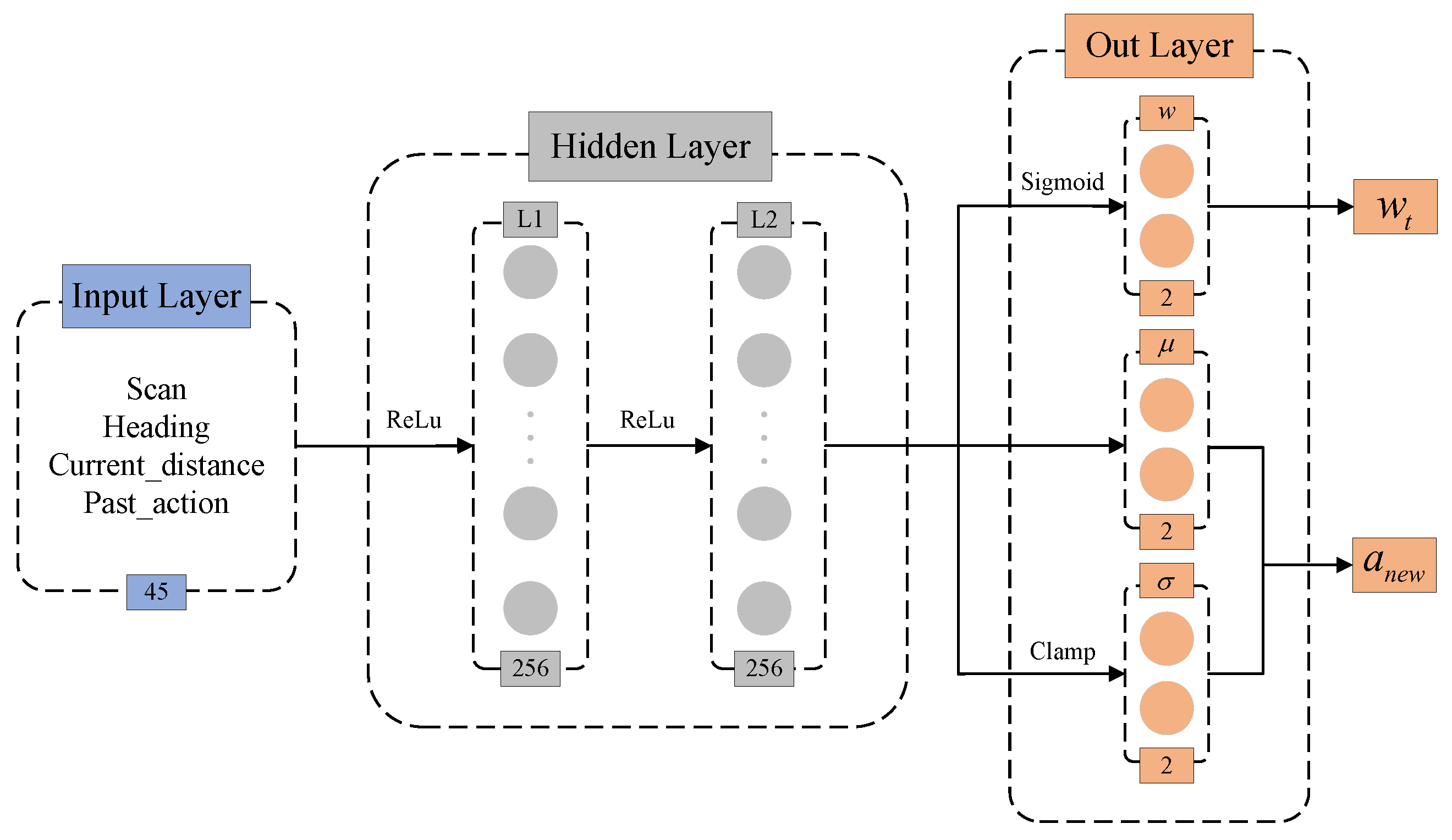
3.1.2. Design of the Fusion Policy Networks
3.1.3. Fusion Policy Networks Transfer Mechanism
3.1.4. Training and Update Process of the Algorithm
3.2. Bio-Inspired Radar Perception Processing
3.2.1. State Space
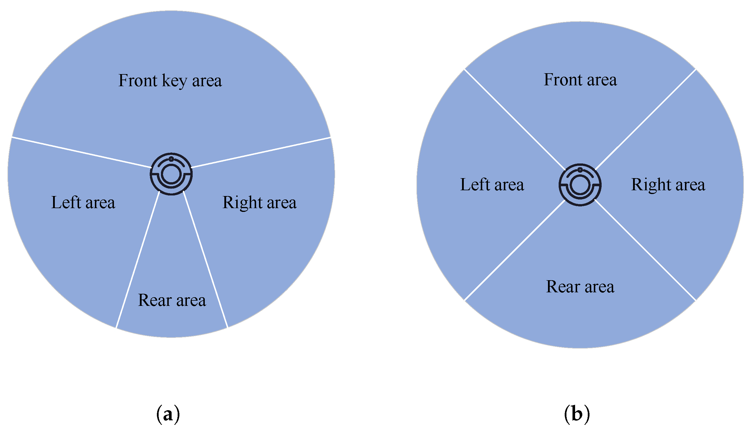
3.2.2. LiDAR Region Segmentation Method
3.2.3. Regional Feature Optimization Method
3.3. Reward Function Based on Invalid Behavior Recognition Mechanism
3.3.1. Reward Function
3.3.2. Invalid Behavior Recognition Mechanism
| Algorithm 1: Pseudo-Code of LT-SAC Algorithm |
 |
4. Experimental Validation
4.1. Experimental Setting
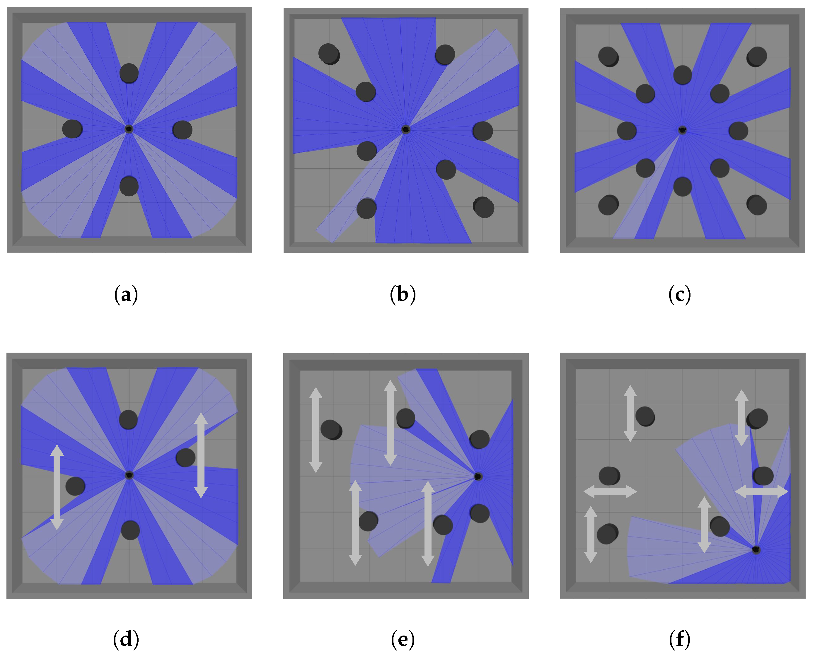
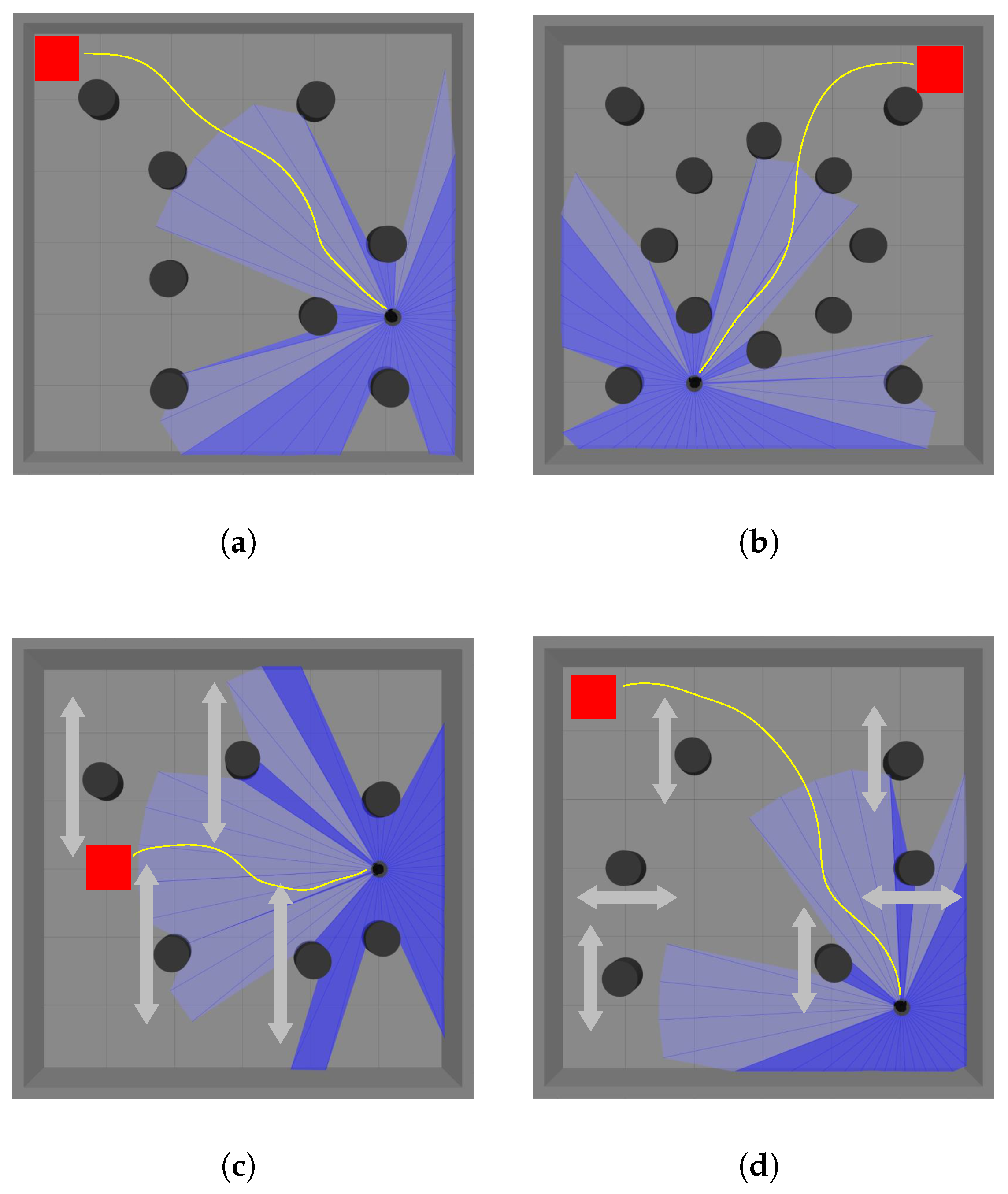
Simulation Scenarios
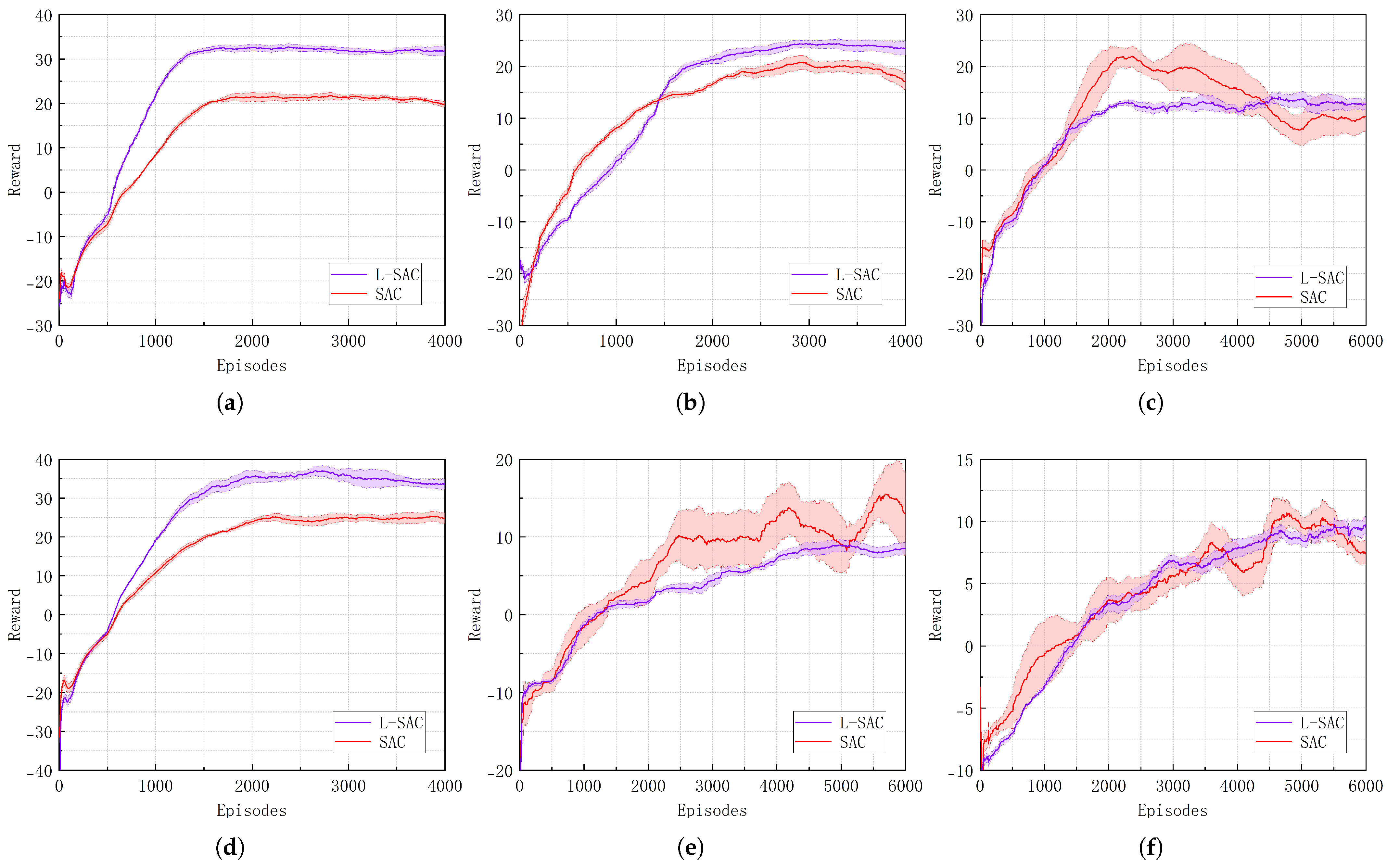
4.2. FPTM Experimental Validation
4.3. BIOM Experimental Validation
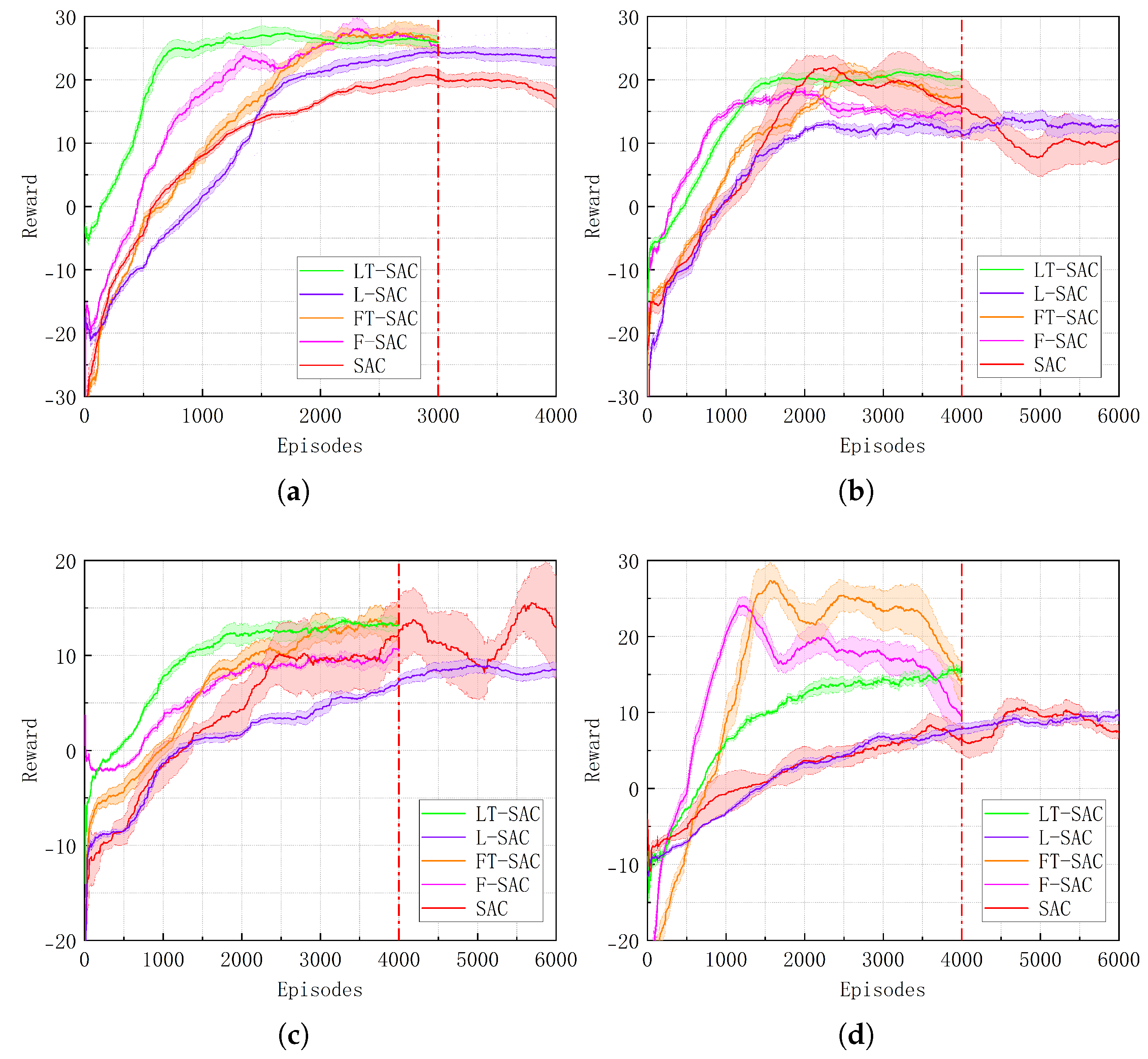
4.4. LT-SAC Experimental Validation
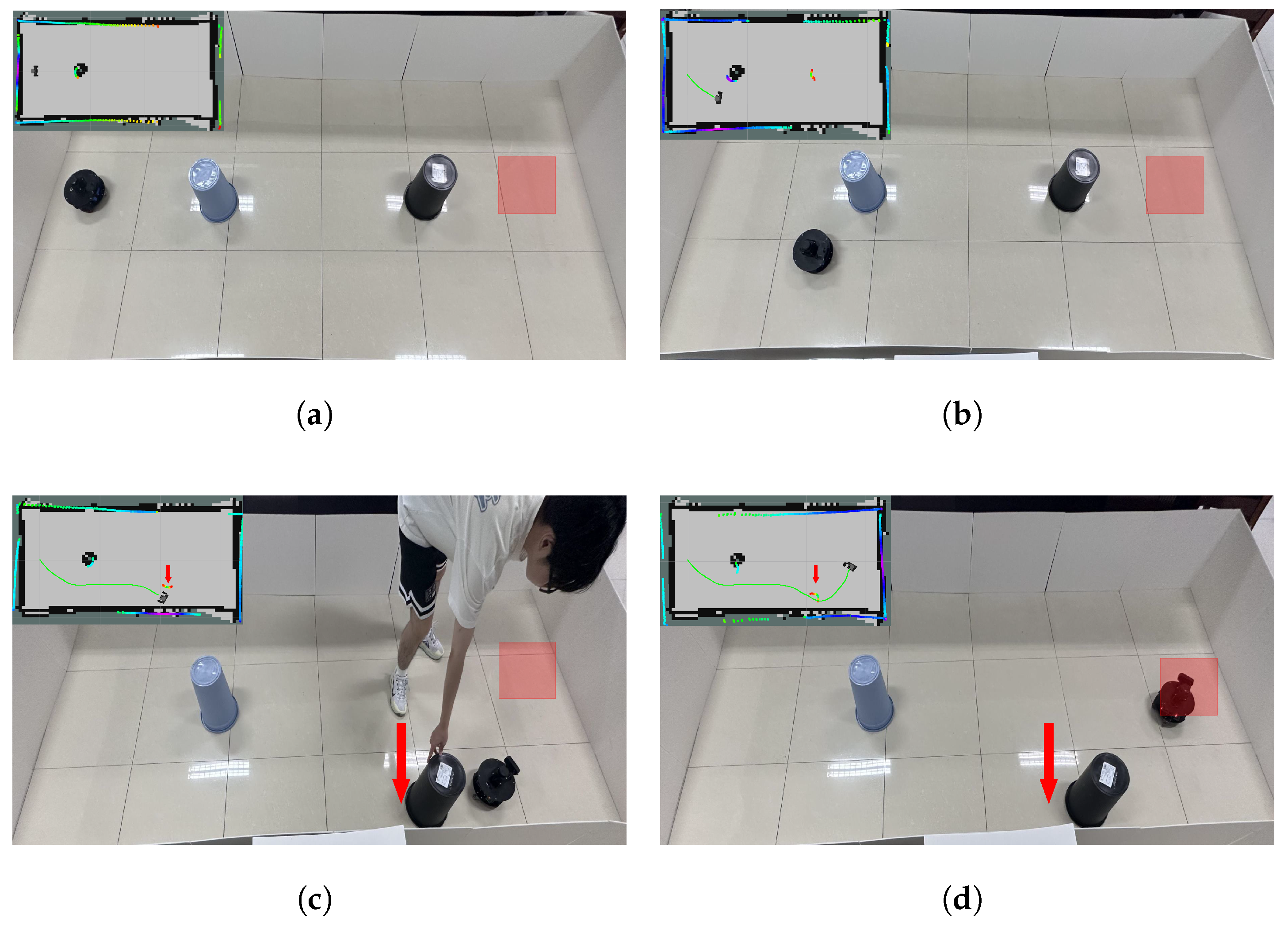
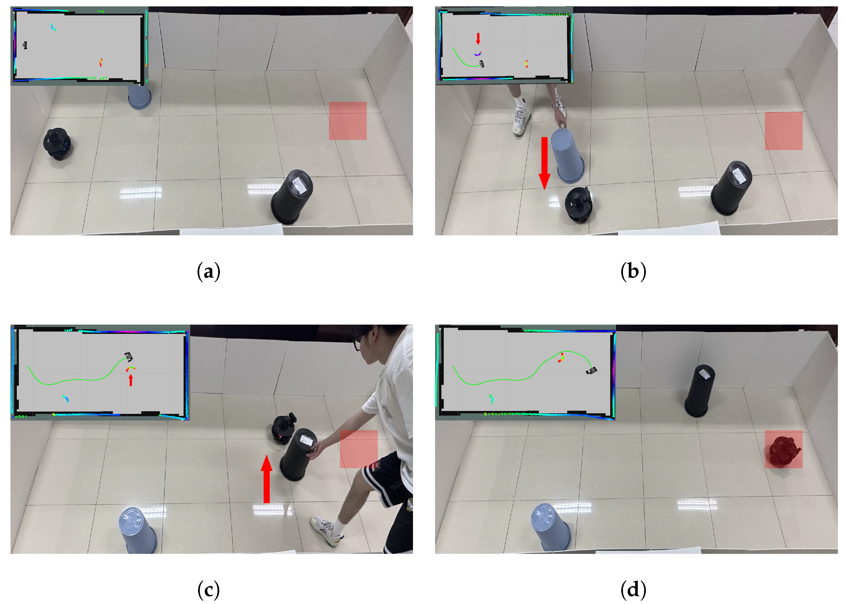
4.5. Actual Scenario Validation
4.5.1. Actual Static Scenario
4.5.2. Actual Dynamic Scenario
5. Conclusions
Author Contributions
Funding
Institutional Review Board Statement
Informed Consent Statement
Data Availability Statement
Conflicts of Interest
Abbreviations
| FPTM | Fusion Policy Networks Transfer Learning Method |
| BIOM | Bio-inspired Perception-driven LiDAR Information Optimization Method |
| IBRM | Invalid Behavior Recognition Mechanism |
| LT-SAC | The SAC algorithm integrated with three core components |
| L-SAC | The SAC algorithm with only BIOM |
| T-SAC | The SAC algorithm with only FPTM |
| FT-SAC | The SAC algorithm based on fine-tuning transfer method |
| F-SAC | The SAC algorithm based on frozen-layer transfer method |
References
- Zhu, X.; Jia, C.; Zhao, J.; Xia, C.; Peng, W.; Huang, J.; Li, L. An Enhanced Artificial Lemming Algorithm and Its Application in UAV Path Planning. Biomimetics 2025, 10, 377. [Google Scholar] [CrossRef]
- Hu, J.; Niu, J.; Zhang, B.; Gao, X.; Zhang, X.; Huang, S. Obstacle Avoidance Strategy and Path Planning of Medical Automated Guided Vehicles Based on the Bionic Characteristics of Antelope Migration. Biomimetics 2025, 10, 142. [Google Scholar] [CrossRef]
- Wang, L.; Liu, G. Research on multi-robot collaborative operation in logistics and warehousing using A3C optimized YOLOv5-PPO model. Front. Neurorobotics 2024, 17, 1329589. [Google Scholar] [CrossRef]
- Kim, S.; Yoon, S.; Cho, J.H.; Kim, D.S.; Moore, T.J.; Free-Nelson, F.; Lim, H. DIVERGENCE: Deep reinforcement learning-based adaptive traffic inspection and moving target defense countermeasure framework. IEEE Trans. Netw. Serv. Manag. 2022, 19, 4834–4846. [Google Scholar] [CrossRef]
- Li, X.; Liang, X.; Wang, X.; Wang, R.; Shu, L.; Xu, W. Deep reinforcement learning for optimal rescue path planning in uncertain and complex urban pluvial flood scenarios. Appl. Soft Comput. 2023, 144, 110543. [Google Scholar] [CrossRef]
- Du, H.; Liu, M.; Liu, N.; Li, D.; Li, W.; Xu, L. Scheduling of Low-Latency Medical Services in Healthcare Cloud with Deep Reinforcement Learning. Tsinghua Sci. Technol. 2024, 30, 100–111. [Google Scholar] [CrossRef]
- Kästner, L.; Marx, C.; Lambrecht, J. Deep-reinforcement-learning-based semantic navigation of mobile robots in dynamic environments. In Proceedings of the 2020 IEEE 16th International Conference on Automation Science and Engineering (CASE), Hong Kong, China, 20–21 August 2020; pp. 1110–1115. [Google Scholar]
- Yan, J.; Zhang, L.; Yang, X.; Chen, C.; Guan, X. Communication-aware motion planning of AUV in obstacle-dense environment: A binocular vision-based deep learning method. IEEE Trans. Intell. Transp. Syst. 2023, 24, 14927–14943. [Google Scholar] [CrossRef]
- Wang, H.; Yu, Y.; Yuan, Q. Application of Dijkstra algorithm in robot path-planning. In Proceedings of the 2011 Second International Conference on Mechanic Automation and Control Engineering, Hohhot, China, 15–17 July 2011; pp. 1067–1069. [Google Scholar]
- Le, A.V.; Prabakaran, V.; Sivanantham, V.; Mohan, R.E. Modified a-star algorithm for efficient coverage path planning in tetris inspired self-reconfigurable robot with integrated laser sensor. Sensors 2018, 18, 2585. [Google Scholar] [CrossRef]
- Duchoň, F.; Babinec, A.; Kajan, M.; Beňo, P.; Florek, M.; Fico, T.; Jurišica, L. Path Planning with Modified a Star Algorithm for a Mobile Robot—ScienceDirect. Procedia Eng. 2014, 96, 59–69. [Google Scholar] [CrossRef]
- Ferguson, D.; Stentz, A. Using interpolation to improve path planning: The Field D* algorithm. J. Field Robot. 2006, 23, 79–101. [Google Scholar] [CrossRef]
- Su, J.; Li, J. Path planning for mobile robots based on genetic algorithms. In Proceedings of the 2013 Ninth International Conference on Natural Computation (ICNC), Shenyang, China, 23–25 July 2013; pp. 723–727. [Google Scholar]
- Miao, C.; Chen, G.; Yan, C.; Wu, Y. Path planning optimization of indoor mobile robot based on adaptive ant colony algorithm. Comput. Ind. Eng. 2021, 156, 107230. [Google Scholar] [CrossRef]
- Ran, M.; Duan, H.; Gao, X.; Mao, Z. Improved particle swarm optimization approach to path planning of amphibious mouse robot. In Proceedings of the 2011 6th IEEE Conference on Industrial Electronics and Applications, Beijing, China, 21–23 June 2011. [Google Scholar]
- Sun, H.; Zhang, W.; Yu, R.; Zhang, Y. Motion planning for mobile robots—Focusing on deep reinforcement learning: A systematic review. IEEE Access 2021, 9, 69061–69081. [Google Scholar] [CrossRef]
- Yang, Y.; Juntao, L.; Lingling, P. Multi-robot path planning based on a deep reinforcement learning DQN algorithm. CAAI Trans. Intell. Technol. 2020, 5, 177–183. [Google Scholar] [CrossRef]
- Wang, W.; Li, L.; Ye, F.; Peng, Y.; Ma, Y. A LARGE-SCALE PATH PLANNING ALGORITHM FOR UNDERWATER ROBOTS BASED ON DEEP REINFORCEMENT LEARNING. Int. J. Robot. Autom. 2024, 39. [Google Scholar] [CrossRef]
- Li, P.; Wang, Y.; Gao, Z. Path planning of mobile robot based on improved td3 algorithm. In Proceedings of the 2022 IEEE International Conference on Mechatronics and Automation (ICMA), Guilin, China, 7–10 August 2022; pp. 715–720. [Google Scholar]
- Haarnoja, T.; Zhou, A.; Abbeel, P.; Levine, S. Soft actor-critic: Off-policy maximum entropy deep reinforcement learning with a stochastic actor. In Proceedings of the International Conference on Machine Learning, ICML 2018, Stockholm, Sweden, 10–15 July 2018; pp. 1861–1870. [Google Scholar]
- Zhu, Z.; Lin, K.; Jain, A.K.; Zhou, J. Transfer learning in deep reinforcement learning: A survey. IEEE Trans. Pattern Anal. Mach. Intell. 2023, 45, 13344–13362. [Google Scholar] [CrossRef] [PubMed]
- Zhuang, F.; Qi, Z.; Duan, K.; Xi, D.; Zhu, Y.; Zhu, H.; Xiong, H.; He, Q. A comprehensive survey on transfer learning. Proc. IEEE 2020, 109, 43–76. [Google Scholar] [CrossRef]
- Wang, H.C.; Huang, S.C.; Huang, P.J.; Wang, K.L.; Teng, Y.C.; Ko, Y.T.; Jeon, D.; Wu, I.C. Curriculum reinforcement learning from avoiding collisions to navigating among movable obstacles in diverse environments. IEEE Robot. Autom. Lett. 2023, 8, 2740–2747. [Google Scholar] [CrossRef]
- Narvekar, S.; Peng, B.; Leonetti, M.; Sinapov, J.; Taylor, M.E.; Stone, P. Curriculum learning for reinforcement learning domains: A framework and survey. J. Mach. Learn. Res. 2020, 21, 1–50. [Google Scholar]
- Du, Y.; Qi, N.; Wang, K.; Xiao, M.; Wang, W. Intelligent reflecting surface-assisted UAV inspection system based on transfer learning. IET Commun. 2024, 18, 214–224. [Google Scholar] [CrossRef]
- Du, Y.; Qi, N.; Li, X.; Xiao, M.; Boulogeorgos, A.A.A.; Tsiftsis, T.A.; Wu, Q. Distributed multi-UAV trajectory planning for downlink transmission: A GNN-enhanced DRL approach. IEEE Wirel. Commun. Lett. 2024, 13, 3578–3582. [Google Scholar] [CrossRef]
- Li, W.; Yue, M.; Shangguan, J.; Jin, Y. Navigation of mobile robots based on deep reinforcement learning: Reward function optimization and knowledge transfer. Int. J. Control. Autom. Syst. 2023, 21, 563–574. [Google Scholar] [CrossRef]
- Bo, L.; Zhang, T.; Zhang, H.; Hong, J.; Liu, M.; Zhang, C.; Liu, B. 3D UAV path planning in unknown environment: A transfer reinforcement learning method based on low-rank adaption. Adv. Eng. Inform. 2024, 62, 102920. [Google Scholar] [CrossRef]
- Wang, Y.; Shen, B.; Nan, Z.; Tao, W. An End-to-End Path Planner Combining Potential Field Method with Deep Reinforcement Learning. IEEE Sens. J. 2024, 24, 26584–26591. [Google Scholar] [CrossRef]
- Zhang, W.; Zhang, Y.; Liu, N.; Ren, K.; Wang, P. IPAPRec: A promising tool for learning high-performance mapless navigation skills with deep reinforcement learning. IEEE/ASME Trans. Mechatron. 2022, 27, 5451–5461. [Google Scholar] [CrossRef]
- de Heuvel, J.; Zeng, X.; Shi, W.; Sethuraman, T.; Bennewitz, M. Spatiotemporal attention enhances lidar-based robot navigation in dynamic environments. IEEE Robot. Autom. Lett. 2024, 9, 4202–4209. [Google Scholar] [CrossRef]
- Ou, Y.; Cai, Y.; Sun, Y.; Qin, T. Autonomous navigation by mobile robot with sensor fusion based on deep reinforcement learning. Sensors 2024, 24, 3895. [Google Scholar] [CrossRef] [PubMed]
- Tan, J. A method to plan the path of a robot utilizing deep reinforcement learning and multi-sensory information fusion. Appl. Artif. Intell. 2023, 37, 2224996. [Google Scholar] [CrossRef]
- Yuan, J.; Lv, M.; Zhang, J. Research on Mobile Robot Path Planning Based on Improved Distributional Reinforcement Learning. In Proceedings of the 2024 43rd Chinese Control Conference (CCC), Kunming, China, 28–31 July 2024; pp. 4357–4362. [Google Scholar]
- Peng, G.; Yang, J.; Li, X.; Khyam, M.O. Deep reinforcement learning with a stage incentive mechanism of dense reward for robotic trajectory planning. IEEE Trans. Syst. Man Cybern. Syst. 2022, 53, 3566–3573. [Google Scholar] [CrossRef]
- Yan, C.; Chen, G.; Li, Y.; Sun, F.; Wu, Y. Immune deep reinforcement learning-based path planning for mobile robot in unknown environment. Appl. Soft Comput. 2023, 145, 110601. [Google Scholar] [CrossRef]
- Sheng, Y.; Liu, H.; Li, J.; Han, Q. UAV Autonomous Navigation Based on Deep Reinforcement Learning in Highly Dynamic and High-Density Environments. Drones 2024, 8, 516. [Google Scholar] [CrossRef]
- Haarnoja, T.; Zhou, A.; Hartikainen, K.; Tucker, G.; Ha, S.; Tan, J.; Kumar, V.; Zhu, H.; Gupta, A.; Abbeel, P.; et al. Soft actor-critic algorithms and applications. arXiv 2018, arXiv:1812.05905. [Google Scholar]
- Koenig, N.; Howard, A. Design and use paradigms for gazebo, an open-source multi-robot simulator. In Proceedings of the 2004 IEEE/RSJ International Conference on Intelligent Robots and Systems (IROS) (IEEE Cat. No. 04CH37566), Sendai, Japan, 28 September–2 October 2004; Volume 3, pp. 2149–2154. [Google Scholar]


| Parameter Name | Symbol | Value |
|---|---|---|
| State Space Dimension | 45 | |
| Action Space Dimension | 2 | |
| Hidden Layer Dimension | 256 | |
| Replay Buffer Size | 50,000 | |
| Training Batch Size | 256 | |
| Discount Factor | 0.99 | |
| Learning Rate | 0.0001 | |
| Soft Update Coefficient | 0.005 | |
| Entropy | 0.2 | |
| Velocity Coefficient | 0.1 | |
| Position Coefficient | 0.1 | |
| Goal Reward | 8 | |
| Collision Penalty | −4 | |
| Penalty of Stagnation | −2 | |
| Stagnation Steps Threshold | N | 4 |
| Scenario | Index | T-SAC | SAC | Improvement (%) |
|---|---|---|---|---|
| (b) | Episodes | 1600 | 3000 | +46.67 |
| Reward | 23.43 | 20.16 | +16.22 | |
| (c) | Episodes | 2100 | – | – |
| Reward | 22.57 | – | – | |
| (e) | Episodes | 2500 | – | – |
| Reward | 12.15 | – | – | |
| (f) | Episodes | 3000 | – | – |
| Reward | 8.47 | – | – |
| Scenario | Index | L-SAC | SAC | Improvement (%) |
|---|---|---|---|---|
| (a) | Episodes | 1500 | 1700 | +11.76 |
| Reward | 32.86 | 22.43 | +46.50 | |
| (b) | Episodes | 2800 | 3000 | +6.67 |
| Reward | 24.54 | 19.12 | +28.35 | |
| (c) | Episodes | 2700 | – | – |
| Reward | 13.46 | – | – | |
| (d) | Episodes | 2000 | 2200 | +9.09 |
| Reward | 34.53 | 24.85 | +38.95 | |
| (e) | Episodes | 4500 | – | – |
| Reward | 8.67 | – | – | |
| (f) | Episodes | 4700 | – | – |
| Reward | 9.94 | – | – |
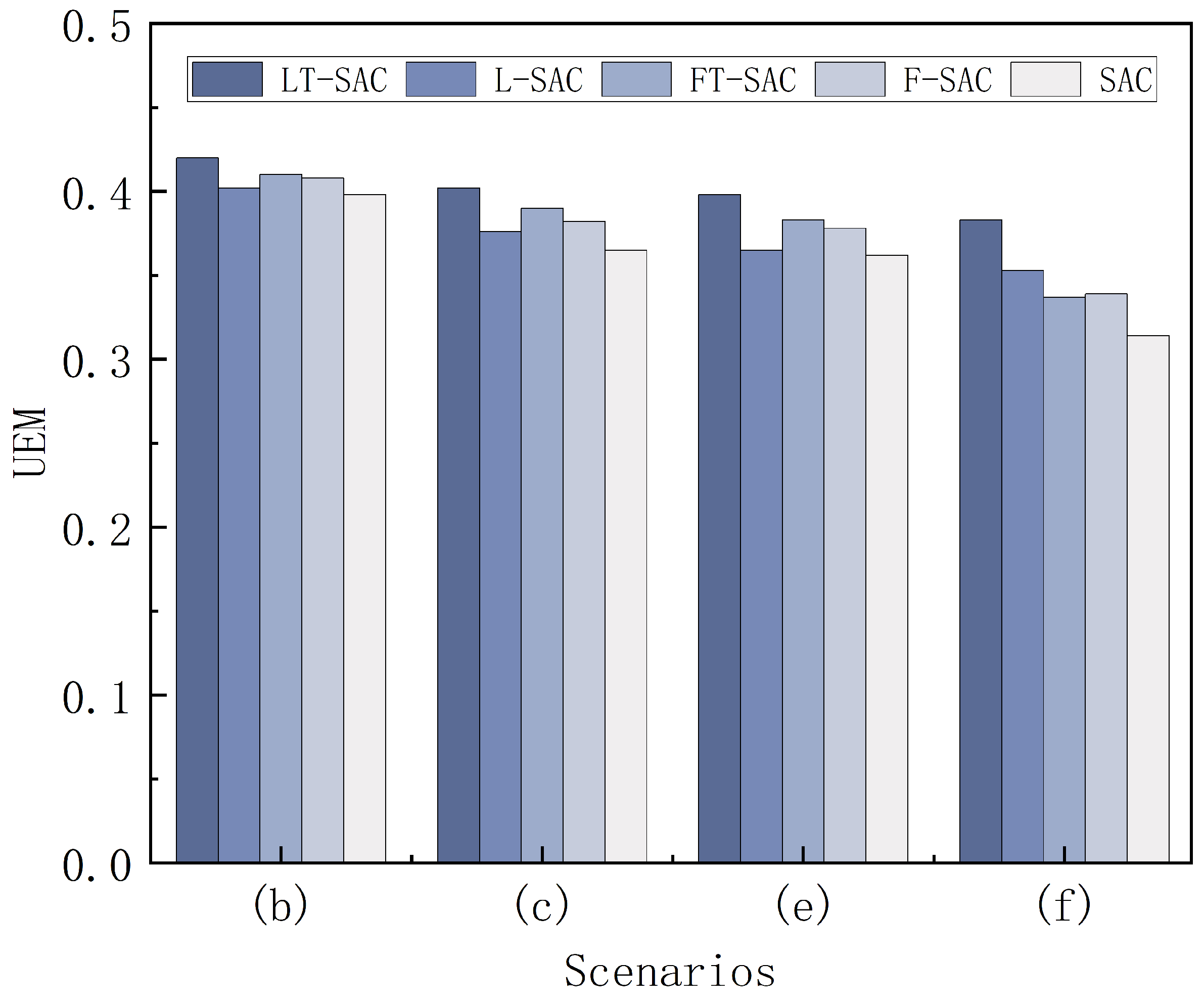
| Scenario | Algorithm | S | L | R | UEM | |
|---|---|---|---|---|---|---|
| (b) | LT-SAC | 0.99 | 5.66 | 1250 | 22.75 | 0.420 |
| L-SAC | 0.91 | 5.72 | 3000 | 19.12 | 0.402 | |
| FT-SAC | 0.94 | 5.70 | 2000 | 22.46 | 0.410 | |
| F-SAC | 0.93 | 5.69 | 2200 | 22.94 | 0.408 | |
| SAC | 0.89 | 5.81 | 3000 | 20.16 | 0.398 | |
| (c) | LT-SAC | 0.90 | 5.47 | 1500 | 20.52 | 0.402 |
| L-SAC | 0.80 | 5.82 | 2700 | 13.46 | 0.376 | |
| FT-SAC | 0.85 | 5.74 | 2500 | 18.37 | 0.390 | |
| F-SAC | 0.82 | 5.62 | 2500 | 15.13 | 0.382 | |
| SAC | 0.74 | 5.93 | 6000 | 15.56 | 0.365 | |
| (e) | LT-SAC | 0.88 | 4.72 | 2000 | 13.75 | 0.398 |
| L-SAC | 0.76 | 4.94 | 4500 | 8.67 | 0.365 | |
| FT-SAC | 0.82 | 5.12 | 3000 | 13.96 | 0.383 | |
| F-SAC | 0.81 | 4.92 | 3000 | 10.13 | 0.378 | |
| SAC | 0.72 | 5.19 | 6000 | 12.74 | 0.362 | |
| (f) | LT-SAC | 0.84 | 6.12 | 2000 | 14.53 | 0.383 |
| L-SAC | 0.73 | 6.84 | 4700 | 9.94 | 0.353 | |
| FT-SAC | 0.61 | 7.36 | 4000 | 20.25 | 0.337 | |
| F-SAC | 0.64 | 7.47 | 4000 | 15.12 | 0.339 | |
| SAC | 0.56 | 7.54 | 6000 | 8.46 | 0.314 |
Disclaimer/Publisher’s Note: The statements, opinions and data contained in all publications are solely those of the individual author(s) and contributor(s) and not of MDPI and/or the editor(s). MDPI and/or the editor(s) disclaim responsibility for any injury to people or property resulting from any ideas, methods, instructions or products referred to in the content. |
© 2025 by the authors. Licensee MDPI, Basel, Switzerland. This article is an open access article distributed under the terms and conditions of the Creative Commons Attribution (CC BY) license (https://creativecommons.org/licenses/by/4.0/).
Share and Cite
Wang, S.; Xu, Z.; Qiao, P.; Yue, Q.; Ke, Y.; Gao, F. Research on Robot Obstacle Avoidance and Generalization Methods Based on Fusion Policy Transfer Learning. Biomimetics 2025, 10, 493. https://doi.org/10.3390/biomimetics10080493
Wang S, Xu Z, Qiao P, Yue Q, Ke Y, Gao F. Research on Robot Obstacle Avoidance and Generalization Methods Based on Fusion Policy Transfer Learning. Biomimetics. 2025; 10(8):493. https://doi.org/10.3390/biomimetics10080493
Chicago/Turabian StyleWang, Suyu, Zhenlei Xu, Peihong Qiao, Quan Yue, Ya Ke, and Feng Gao. 2025. "Research on Robot Obstacle Avoidance and Generalization Methods Based on Fusion Policy Transfer Learning" Biomimetics 10, no. 8: 493. https://doi.org/10.3390/biomimetics10080493
APA StyleWang, S., Xu, Z., Qiao, P., Yue, Q., Ke, Y., & Gao, F. (2025). Research on Robot Obstacle Avoidance and Generalization Methods Based on Fusion Policy Transfer Learning. Biomimetics, 10(8), 493. https://doi.org/10.3390/biomimetics10080493