
Approach to Semantic Visual SLAM for Bionic Robots Based on Loop Closure Detection with Combinatorial Graph Entropy in Complex Dynamic Scenes


Abstract
1. Introduction
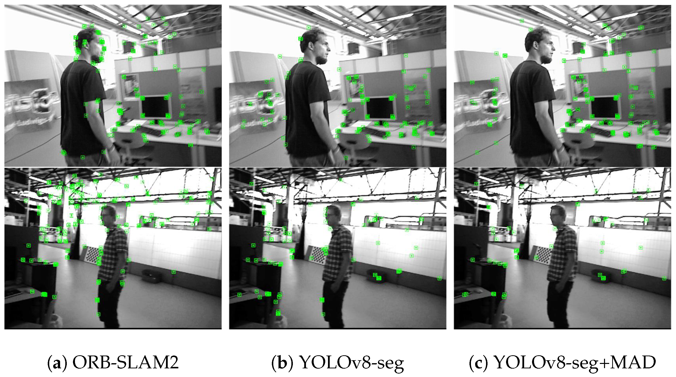
- Based on the segmentation results of YOLOv8-seg, the feature points at the edges of dynamic objects are quickly and accurately judged by calculating the MAD of the depth of the pixel points, which effectively suppresses the influence of dynamic objects on pose estimation.
- A high-quality keyframe selection strategy is constructed by utilizing the semantic information, the average coordinates of semantic objects, and the degree of change in feature point dense areas.
- According to the distribution of feature points, representation points and semantic nodes, a graph structure corresponding to the scene structure of the keyframe is constructed, and then the similarity comparison of two keyframes is realized by calculating their graph entropy, effectively improving the accuracy of loop closure detection.
- A closed-loop similarity calculation method based on scene structure is constructed to determine whether to use only the unweighted graph or both the unweighted graph and the Shannon entropy-based weighted graph, which effectively improves the adaptability of the loop closure detection in different complex scenes.
2. Related Work
2.1. Bionic Robot
2.2. SLAM in Dynamic Scenes
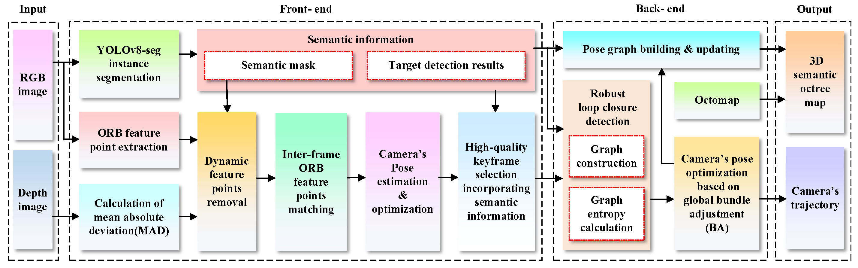
3. Framework and Methods
3.1. Dynamic Feature Elimination
3.2. High-Quality Keyframe Selection
3.3. Loop Closure Detection with Combinatorial Graph Entropy
3.3.1. Graph Construction
- Similarity pre-judgmentFirstly, we define a semantic vector containing n components for the current frame and the candidate frame , respectively, i.e.,where and denote the number of occurrences of the i-th semantic entity in the current frame and candidate frames, respectively. Then, we calculate the cosine similarity between the vectors and , i.e.,According to the calculation result of Equation (19), an closer to 1 indicates that the semantic vectors in the two frames are more similar; in this case, using only the unweighted graph can complete the correct judgment. If is less than a similarity threshold , it indicates that the static background of the two frames has undergone significant changes, but it cannot be determined whether they are the same scene or not. In this case, it is necessary to combine the unweighted image and the weighted image to calculate the similarity.
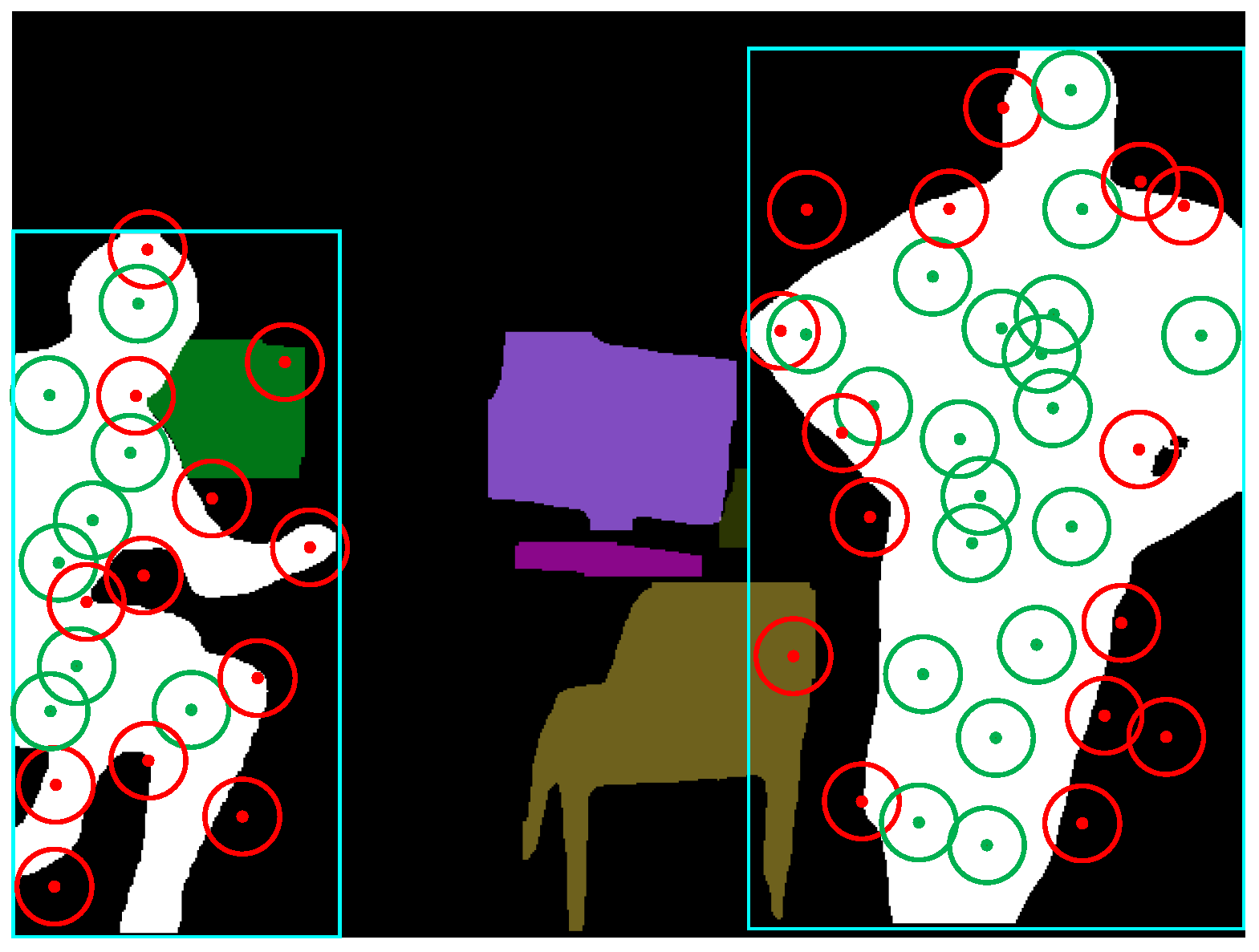
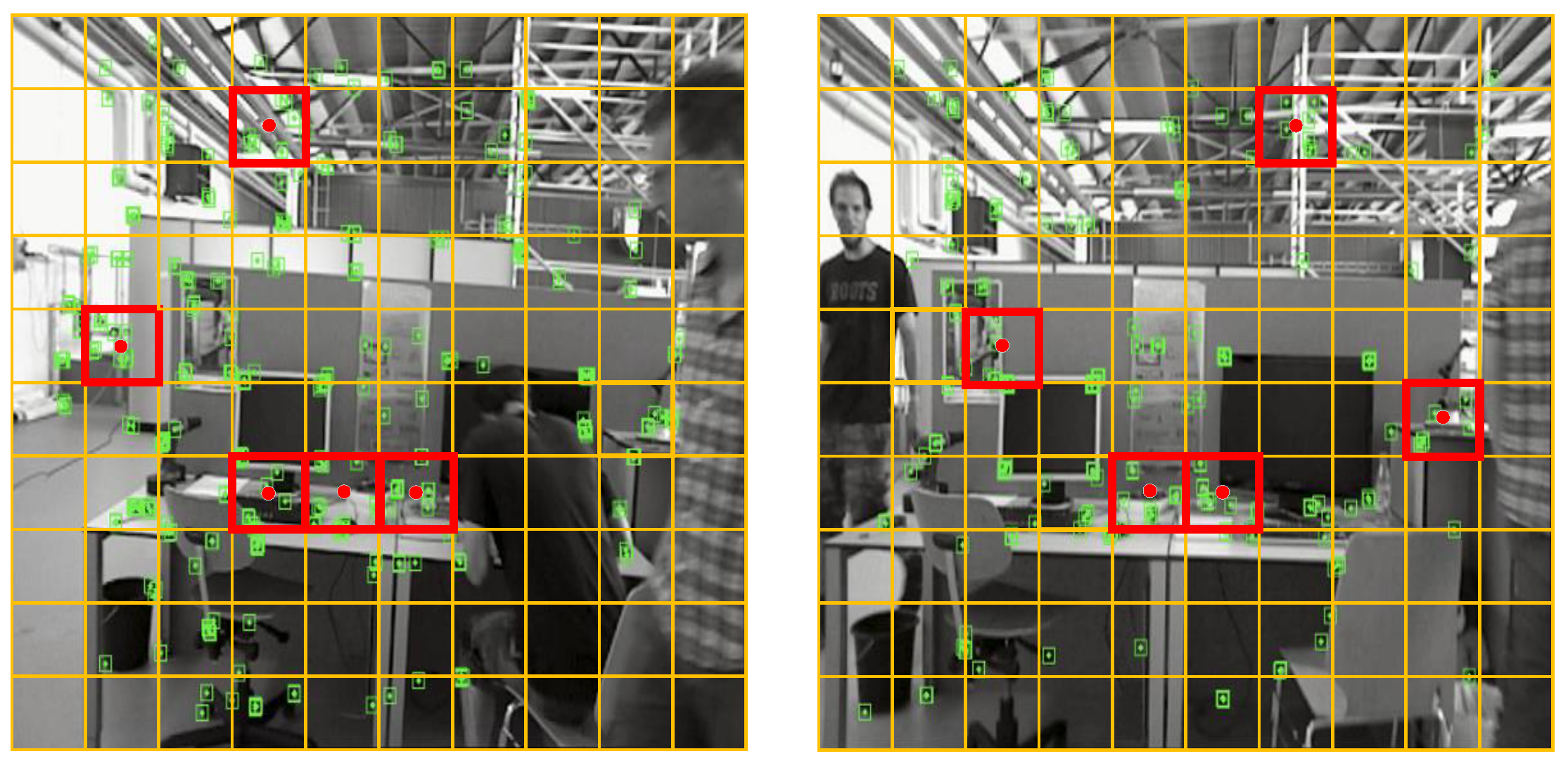
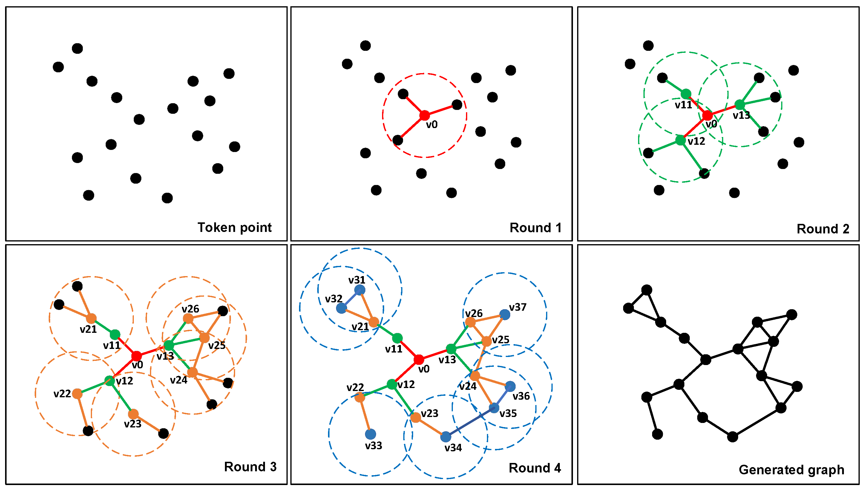
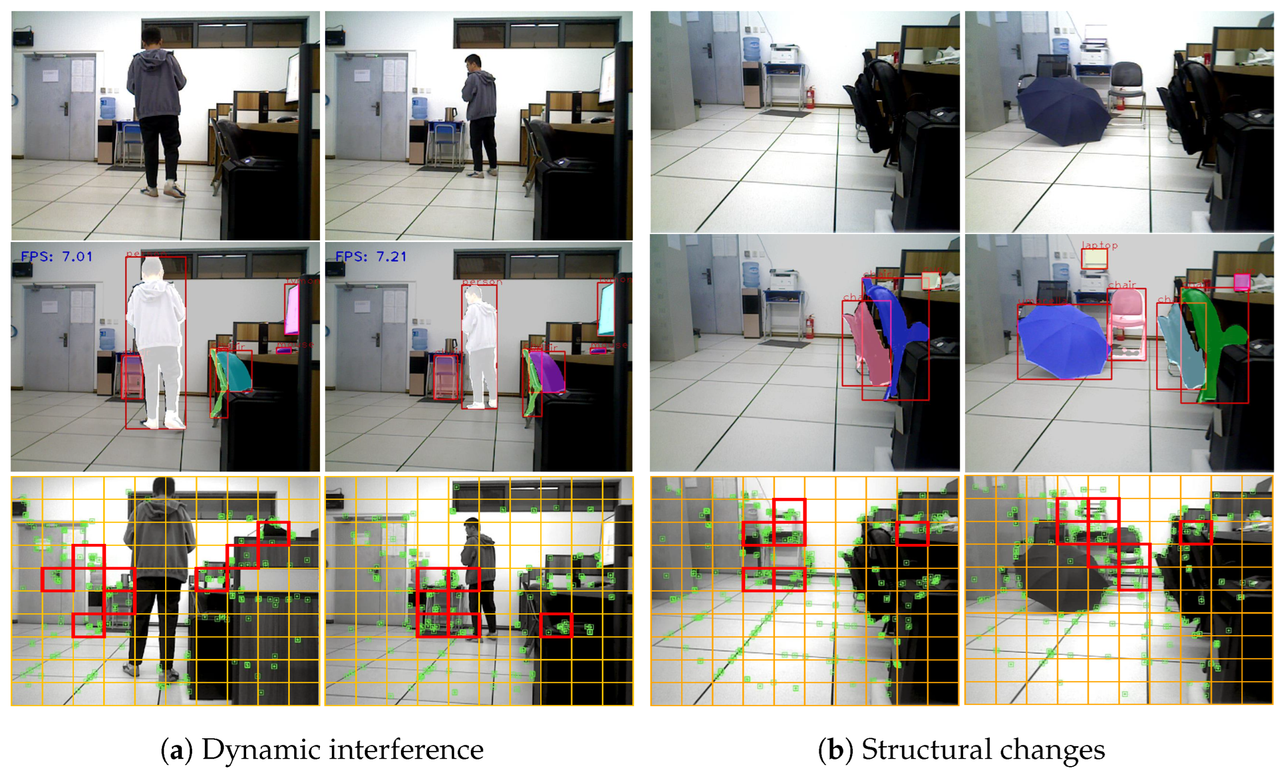
- Representative point determinationTypically, when dynamic objects appear in the field of view (FOV), the distribution of feature points in the extracted scene image is undoubtedly disturbed. Hence, before performing similarity calculation, it is necessary to combine the dynamic masks in the current frame and candidate frames to screen out all stable feature points in the two images. More specifically, assuming is any feature point in the current frame with a pixel coordinate of , if the dynamic masks of both the current and candidate frames do not contain this feature point, then is referred to as a stability feature point.After selecting all the stability feature points, we uniformly divide and into rectangular regions and set the size of the length and width of each region to one-tenth of the length and width of the image. Then, we count the number of stability feature points within each patch. If is greater than the threshold , the feature points in the region are considered too dense, and the center point of the patch is selected as the “representation point”. When performing the graph structure construction, the characterization points are used as nodes of the graph, while the feature points within their respective patches do not participate in the construction of the graph structure, but feature points within other non-dense patches need to participate as nodes in the construction of the graph structure. As shown in Figure 5, since the number of feature points in the red box is greater than the set threshold, they are considered as dense blocks, and the center coordinates of these blocks are recorded as the coordinates of the representation points.
- Graph structure generationA complete graph structure consists of nodes and edges, and in the case of a weighted graph, the weights of the paths need to be set. To accurately represent the similarity between two images, the connection strategy between nodes needs to ensure that the same scene is not affected by the observation perspective. Otherwise, the same image may have different constructed graph structures due to different observation perspectives. In our case, representation points, feature points in non-dense regions, and the centers of semantic entities (i.e., semantic nodes) together form the nodes of the graph.To connect the nodes to form a graph structure, we first set a “” for each node, with at the initial moment, and set the search radius R. Then, the node closest to the center of the image is taken as the starting node , and is connected to the nodes within the search radius R, with as the center of the connection; that is, let the coordinates of be , and the coordinates of any node in the image be . If the following relationship is satisfied, a connection is established .For the search, if no other point is searched within R, that is, no connection is successfully established, the search radius of the node is expanded to , as follows, until a connection is established.In this way, the first round of connections can be completed.The second round of concatenation is sequentially centered on the node that was concatenated in the first round and is searched and concatenated according to the above strategy. Herein, to prevent the graph structure constructed in the case of too sparse keypoints from being too simple, we do not set a threshold for the search radius during the first two rounds of connection.Starting from the third round of connection, each round of the connection process takes the node that was connected in the previous round as the center of connection, and any two points are connected only once. Furthermore, to prevent the search radius from being too large and causing too many connections at the edges, the search radius is restricted to expand up to only from the third round onward.After completing the graph construction, we further determine whether there are any points in the graph that are not involved in the graph construction and, if so, find the nodes in the constructed graph that have the shortest Euclidean distances from these points and connect them. It should be noted that, when a node is successfully connected, it is necessary to determine whether its is equal to 0. If , the node will be used as the center of the connection for the next search process, and its will be set to 1. Figure 6 demonstrates a complete connection process.
3.3.2. Graph Entropy Calculation
- When it is necessary to use the graph entropy of an unweighted graph, inspired by the work [44], we construct the degree-degree correlation indices corresponding to the two graph structures and , respectively, as follows:where is a scaling constant; and denote a node in and , respectively; and denote the number of nodes in and , respectively.The graph entropy indicator is an information function reflecting the degree-to-degree relationship between nodes. For the graph structure of , the calculation of the graph entropy indicator is as follows:If the following hold, one can get .where denotes the diameter of and the connotation of can be found in [43,44]. The node with the shortest path length j from can be represented aswhere denotes the node in with path length j to , i.e., j-sphere [43]. The shortest paths from to the node in can be represented asIt should be noted that may have multiple shortest paths when retrieving each node in . In this case, we choose the case where has the shortest total path after connecting with all the nodes in [43]. is the sum of the differences in degrees between adjacent elements in set , i.e.,where denotes the degree of the node.
- When it is necessary to use the graph entropy of a weighted graph, assuming that the weighted graphs generated by and are as follows:where the weights and denote the set of Euclidean distances between the two endpoints corresponding to all the paths in and , respectively. In this case, we use Shannon entropy to calculate the graph entropy of the two graphs [45]. Herein, the Shannon entropies of and are defined as follows:where , denote the edge of and the edge of , respectively.Compared with the unweighted graph, the weighted graph introduces the distance between the nodes as the weights of the paths when performing the similarity calculation, which can reflect the change in the Euclidean distance between the nodes due to the change in depth to a certain extent. Therefore, the weighted graph is more suitable for loop closure detection in the case of large changes in scene structure.
3.3.3. Similarity Calculation
- When only unweighted graphs need to be used, the graph entropies of and are the corresponding degree–degree correlation indices, respectively, i.e.,Hence, the final graph entropy similarity score is as follows:
- When it is necessary to use both unweighted and weighted graphs, the similarity scores of the corresponding unweighted graphs of and are calculated as follows:Subsequently, let the graph entropies of and be the corresponding Shannon entropies, respectively, i.e.,The similarity scores of the corresponding weighted graphs of and are calculated as follows:Further, the following combinatorial graph entropy similarity score is obtained by evaluating the two similarity scores together:Finally, we utilize the calculated as the graph entropy similarity score for and . In this paper, in the case of using both unweighted and weighted graphs, .

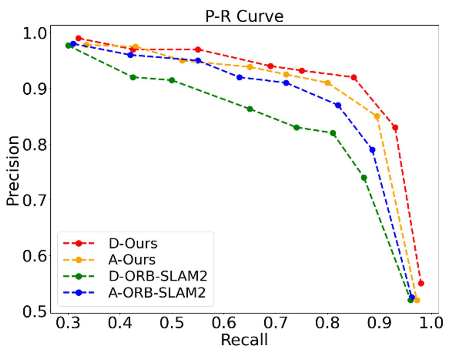
4. Simulation and Experimental Results
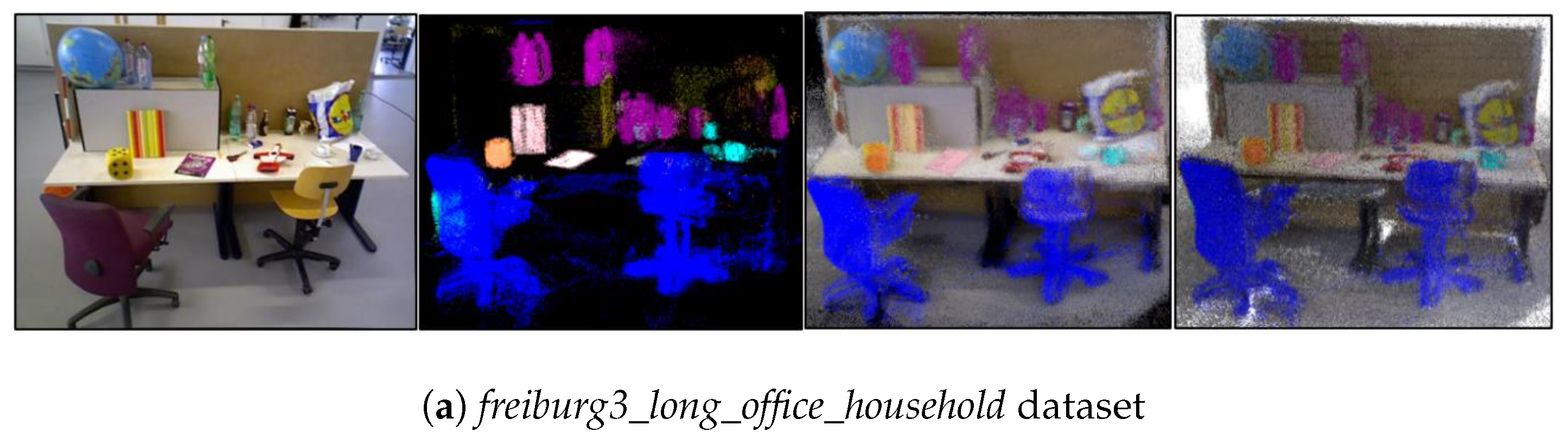
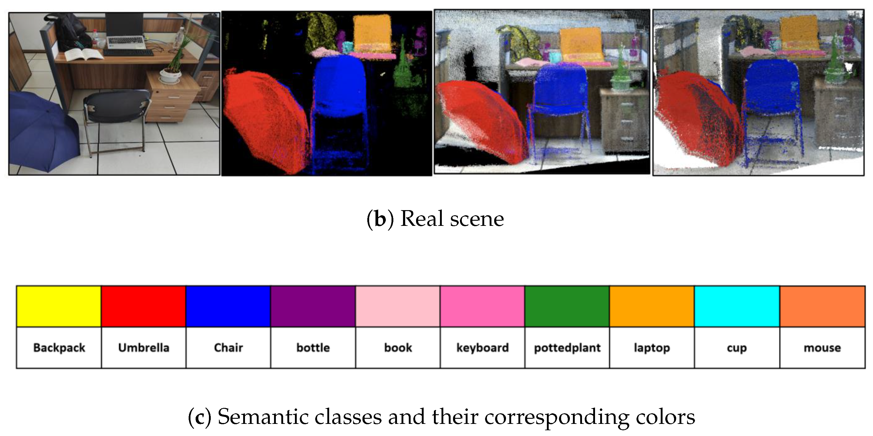
4.1. Simulation Studies Under the TUM Dataset
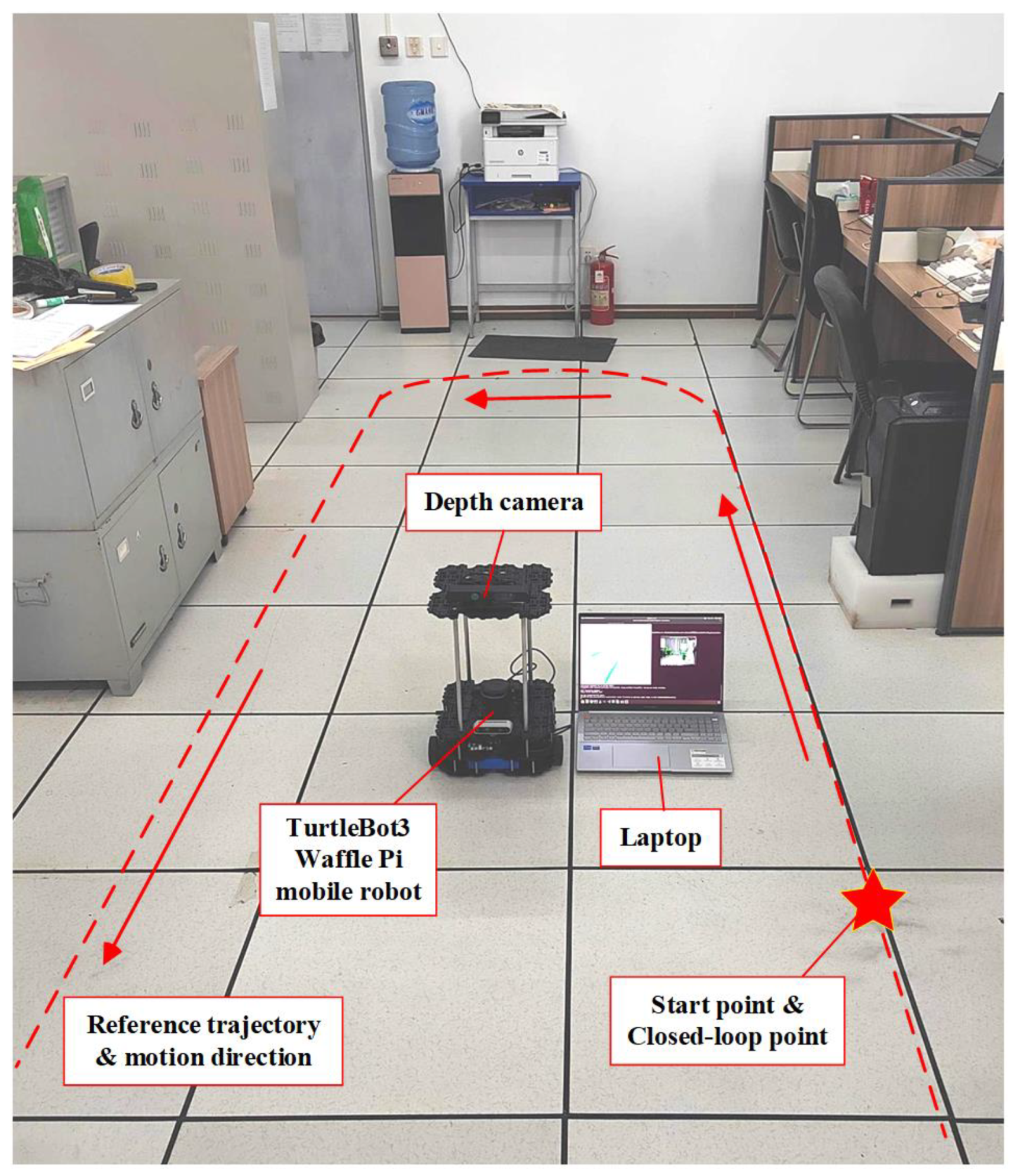
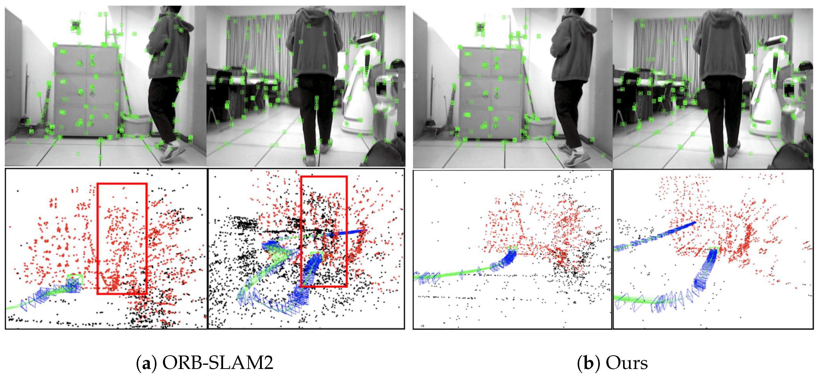
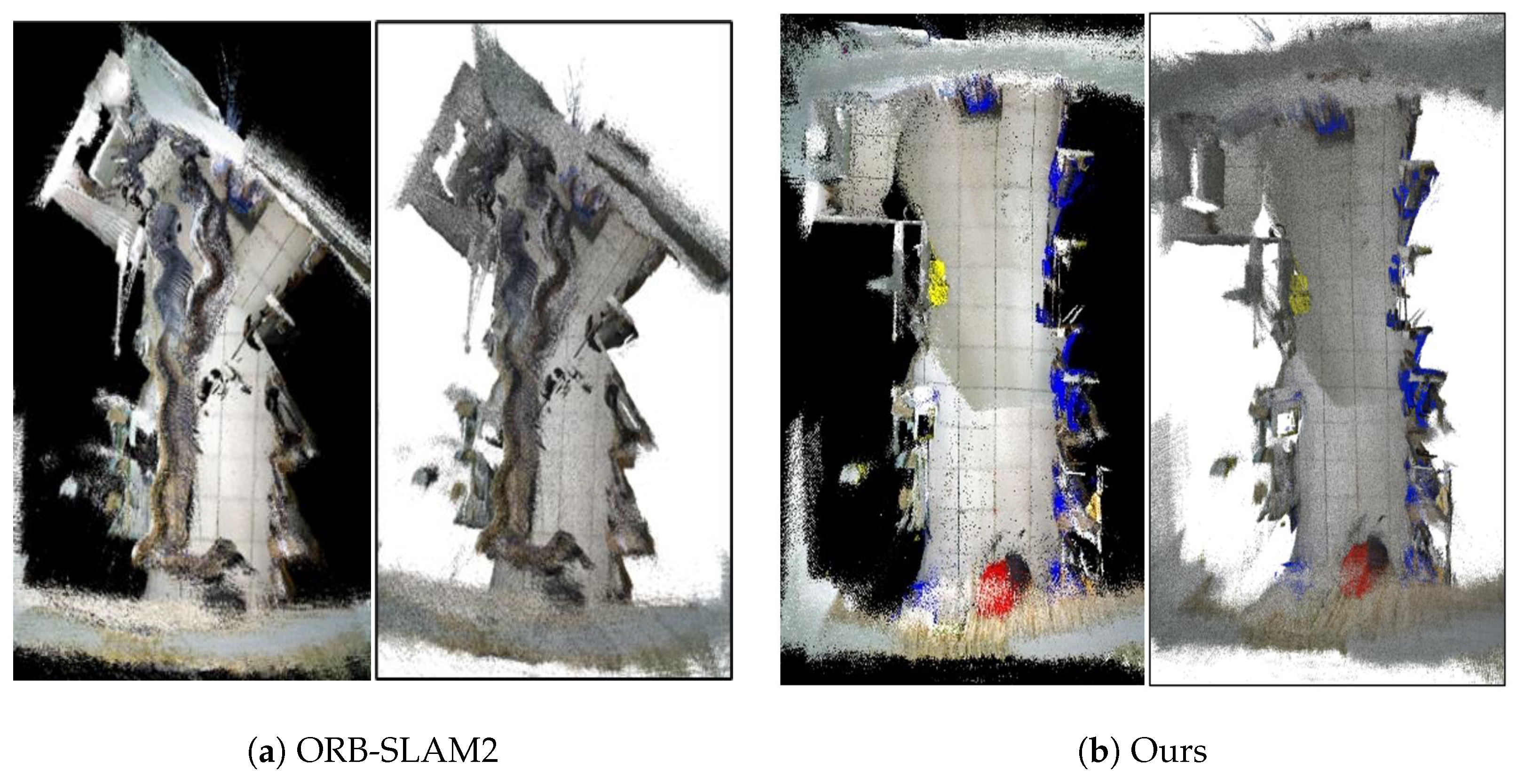
4.2. Experimental Testing with a Mobile Robot
5. Conclusions and Future Work
Author Contributions
Funding
Institutional Review Board Statement
Informed Consent Statement
Data Availability Statement
Conflicts of Interest
Abbreviations
| CGE-vSLAM | The proposed algorithm |
| vSLAM | Visual simultaneous localization and mapping |
| ORB | Oriented Fast and Rotated Brief |
| MAD | Mean Absolute Deviation |
| BOW | Bag of Words |
| BA | Bundle Adjustment |
| PCL | Point Cloud Library |
| ATE | Absolute Trajectory Error |
| RTE | Relative Translation Error |
| RMSE | Root Mean Square Error |
References
- Li, X.; Hu, Y.; Jie, Y.; Zhao, C.; Zhang, Z. Dual-Frequency LiDAR for Compressed Sensing 3D Imaging Based on All-Phase Fast Fourier Transform. J. Opt. Photonics Res. 2024, 1, 74–81. [Google Scholar] [CrossRef]
- Qin, Y.; Yu, H. A review of visual SLAM with dynamic objects. Ind.-Robot.-Int. J. Robot. Res. Appl. 2023, 50, 1000–1010. [Google Scholar] [CrossRef]
- Rosen, D.M.; Doherty, K.J.; Espinoza, A.T.; Leonard, J.J. Advances in Inference and Representation for Simultaneous Localization and Mapping. Annu. Rev. Control. Robot. Auton. Syst. 2021, 4, 215–242. [Google Scholar] [CrossRef]
- Mur-Artal, R.; Tardos, J.D. ORB-SLAM2: An Open-Source SLAM System for Monocular, Stereo, and RGB-D Cameras. IEEE Trans. Robot. 2017, 33, 1255–1262. [Google Scholar] [CrossRef]
- Engel, J.; Schps, T.; Cremers, D. LSD-SLAM: Large-scale direct monocular SLAM. In Proceedings of the 13th European Conference, Zurich, Switzerland, 6–12 September 2014. [Google Scholar]
- Pumarola, A.; Vakhitov, A.; Agudo, A.; Sanfeliu, A.; Moreno-Noguer, F. PL-SLAM: Real-time monocular visual SLAM with points and lines. In Proceedings of the 2017 IEEE International Conference on Robotics and Automation (ICRA), Singapore, 29 May–3 June 2017. [Google Scholar]
- Li, Z.; Xu, B.; Wu, D.; Zhao, K.; Chen, S.; Lu, M.; Cong, J. A YOLO-GGCNN based grasping framework for mobile robots in unknown environments. Expert Syst. Appl. 2023, 225, 119993. [Google Scholar] [CrossRef]
- Wang, Y.; Tian, Y.; Chen, J.; Xu, K.; Ding, X. A Survey of Visual SLAM in Dynamic Environment: The Evolution From Geometric to Semantic Approaches. IEEE Trans. Instrum. Meas. 2024, 73, 2523221. [Google Scholar] [CrossRef]
- Dai, W.; Zhang, Y.; Li, P.; Fang, Z.; Scherer, S. RGB-D SLAM in Dynamic Environments Using Point Correlations. IEEE Trans. Pattern Anal. Mach. Intell. 2022, 44, 373–389. [Google Scholar] [CrossRef]
- Ul Islam, Q.; Ibrahim, H.; Chin, P.K.; Lim, K.; Abdullah, M.Z.; Khozaei, F. ARD-SLAM: Accurate and robust dynamic SLAM using dynamic object identification and improved multi-view geometrical approaches. Displays 2024, 82, 102654. [Google Scholar] [CrossRef]
- Wang, C.; Luo, B.; Zhang, Y.; Zhao, Q.; Yin, L.; Wang, W.; Su, X.; Wang, Y.; Li, C. DymSLAM: 4D Dynamic Scene Reconstruction Based on Geometrical Motion Segmentation. IEEE Robot. Autom. Lett. 2021, 6, 550–557. [Google Scholar] [CrossRef]
- Zheng, Z.; Lin, S.; Yang, C. RLD-SLAM: A Robust Lightweight VI-SLAM for Dynamic Environments Leveraging Semantics and Motion Information. IEEE Trans. Ind. Electron. 2024, 71, 14328–14338. [Google Scholar] [CrossRef]
- Canovas, B.; Rombaut, M.; Negre, A.; Pellerin, D.; Olympieff, S. Speed and Memory Efficient Dense RGB-D SLAM in Dynamic Scenes. In Proceedings of the 2020, IEEE International Conference on Intelligent Robots and Systems, Las Vegas, NV, USA, 24 October 2020–24 January 2021; pp. 4996–5001. [Google Scholar] [CrossRef]
- Liu, Y.; Zhou, Z. Optical Flow-Based Stereo Visual Odometry with Dynamic Object Detection. IEEE Trans. Comput. Soc. Syst. 2023, 10, 3556–3568. [Google Scholar] [CrossRef]
- Wang, H.; Zhang, G.; Cao, H.; Hu, K.; Wang, Q.; Deng, Y.; Gao, J.; Tang, Y. Geometry-Aware 3D Point Cloud Learning for Precise Cutting-Point Detection in Unstructured Field Environments. J. Field Robot. 2025, early view.
- Yi, H.; Liu, B.; Zhao, B.; Liu, E. Small Object Detection Algorithm Based on Improved YOLOv8 for Remote Sensing. IEEE J. Sel. Top. Appl. Earth Obs. Remote. Sens. 2024, 17, 1734–1747. [Google Scholar] [CrossRef]
- Shi, S.; Yang, F.; Fan, S.; Xu, Z. Research on the movement pattern and kinematic model of the hindlegs of the water boatman. Bioinspir. Biomimetics 2025, 20, 016027. [Google Scholar] [CrossRef]
- Tan, T.; Yu, L.; Guo, K.; Wang, X.; Qiao, L. Biomimetic Robotic Remora with Hitchhiking Ability: Design, Control and Experiment. IEEE Robot. Autom. Lett. 2024, 9, 11505–11512. [Google Scholar] [CrossRef]
- Qing, X.; Wang, Y.; Xia, Z.; Liu, S.; Mazhar, S.; Zhao, Y.; Pu, W.; Qiao, G. The passive recording of the click trains of a beluga whale (Delphinapterus leucas) and the subsequent creation of a bio-inspired echolocation model. Bioinspir. Biomimetics 2024, 20, 016019. [Google Scholar] [CrossRef]
- Zhu, C.; Zhou, C.; Zou, Q.; Fan, J.; Zhang, Z.; Ou, Y.; Wang, J. Optimization of a passive roll absorber for robotic fish based on tune mass damper. Bioinspir. Biomimetics 2024, 20, 016011. [Google Scholar] [CrossRef]
- Godon, S.; Ristolainen, A.; Kruusmaa, M. Robotic feet modeled after ungulates improve locomotion on soft wet grounds. Bioinspir. Biomimetics 2024, 19, 066009. [Google Scholar] [CrossRef] [PubMed]
- Leung, B.; Gorb, S.; Manoonpong, P. Nature’s All-in-One: Multitasking Robots Inspired by Dung Beetles. Adv. Sci. 2024, 11, 2408080. [Google Scholar] [CrossRef]
- Kalibala, A.; Nada, A.A.; Ishii, H.; El-Hussieny, H. Dynamic modelling and predictive position/force control of a plant-inspired growing robot. Bioinspir. Biomimetics 2024, 20, 016005. [Google Scholar] [CrossRef]
- Shin, W.D.; Phan, H.V.; Daley, M.A.; Ijspeert, A.J.; Floreano, D. Fast ground-to-air transition with avian-inspired multifunctional legs. Nature 2024, 636, 86–91. [Google Scholar] [CrossRef]
- Xie, Y.; Li, Z.; Song, L.; Zhao, J. A bio-inspired looming detection for stable landing in unmanned aerial vehicles. Bioinspir. Biomimetics 2024, 20, 016007. [Google Scholar] [CrossRef] [PubMed]
- Wang, L.; Zhang, H.; Zhang, L.; Song, B.; Sun, Z.; Zhang, W. Analysis and actuation design of a novel at-scale 3-DOF biomimetic flapping-wing mechanism inspired by flying insects. Bioinspir. Biomimetics 2024, 20, 016015. [Google Scholar] [CrossRef]
- Liu, Z.; Xue, Y.; Zhao, J.; Yin, W.; Zhang, S.; Li, P.; He, B. A Multi-Strategy Siberian Tiger Optimization Algorithm for Task Scheduling in Remote Sensing Data Batch Processing. Biomimetics 2024, 9, 678. [Google Scholar] [CrossRef]
- Liang, H.; Hu, W.; Gong, K.; Dai, J.; Wang, L. Solving UAV 3D Path Planning Based on the Improved Lemur Optimizer Algorithm. Biomimetics 2024, 9, 654. [Google Scholar] [CrossRef]
- Gengbiao, C.; Hanxiao, W.; Lairong, Y. Design, modeling and validation of a low-cost linkage-spring telescopic rod-slide underactuated adaptive robotic hand. Bioinspir. Biomimetics 2024, 20, 016026. [Google Scholar] [CrossRef]
- Lapresa, M.; Lauretti, C.; Cordella, F.; Reggimenti, A.; Zollo, L. Reproducing the caress gesture with an anthropomorphic robot: A feasibility study. Bioinspir. Biomimetics 2024, 20, 016010. [Google Scholar] [CrossRef] [PubMed]
- Guo, Y.; Zhao, Q.; Li, T.; Mao, Q. Masticatory simulators based on oral physiology in food research: A systematic review. J. Texture Stud. 2024, 55, e12864. [Google Scholar] [CrossRef] [PubMed]
- Zhang, Y.; Ge, Q.; Wang, Z.; Qin, Y.; Wu, Y.; Wang, M.; Shi, M.; Xue, L.; Guo, W.; Zhang, Y.; et al. Extracorporeal closed-loop respiratory regulation for patients with respiratory difficulty using a soft bionic robot. IEEE Trans. Biomed. Eng. 2024, 71, 2923–2935. [Google Scholar] [CrossRef] [PubMed]
- Bescos, B.; Facil, J.M.; Civera, J.; Neira, J. DynaSLAM: Tracking, Mapping, and Inpainting in Dynamic Scenes. IEEE Robot. Autom. Lett. 2018, 3, 4076–4083. [Google Scholar] [CrossRef]
- Wei, Y.; Zhou, B.; Duan, Y.; Liu, J.; An, D. DO-SLAM: Research and application of semantic SLAM system towards dynamic environments based on object detection. Appl. Intell. 2023, 53, 30009–30026. [Google Scholar] [CrossRef]
- Li, J.; Luo, J. YS-SLAM: YOLACT plus plus based semantic visual SLAM for autonomous adaptation to dynamic environments of mobile robots. Complex Intell. Syst. 2024, 10, 5771–5792. [Google Scholar] [CrossRef]
- Liu, H.; Luo, J. YES-SLAM: YOLOv7-enhanced-semantic visual SLAM for mobile robots in dynamic scenes. Meas. Sci. Technol. 2024, 35, 035117. [Google Scholar] [CrossRef]
- Wu, W.; Guo, L.; Gao, H.; You, Z.; Liu, Y.; Chen, Z. YOLO-SLAM: A semantic SLAM system towards dynamic environment with geometric constraint. Neural Comput. Appl. 2022, 34, 6011–6026. [Google Scholar] [CrossRef]
- Xiao, L.; Wang, J.; Qiu, X.; Rong, Z.; Zou, X. Dynamic-SLAM: Semantic monocular visual localization and mapping based on deep learning in dynamic environment. Robot. Auton. Syst. 2019, 117, 1–16. [Google Scholar] [CrossRef]
- Cheng, S.; Sun, C.; Zhang, S.; Zhang, D. SG-SLAM: A Real-Time RGB-D Visual SLAM Toward Dynamic Scenes With Semantic and Geometric Information. IEEE Trans. Instrum. Meas. 2023, 72, 7501012. [Google Scholar] [CrossRef]
- Zhang, T.; Zhang, H.; Li, Y.; Nakamura, Y.; Zhang, L. FlowFusion: Dynamic Dense RGB-D SLAM Based on Optical Flow. In Proceedings of the 2020 IEEE International Conference on Robotics and Automation ICRA, Paris, France, 31 May–15 June 2020; pp. 7322–7328. [Google Scholar] [CrossRef]
- Yan, Z.; Chu, S.; Deng, L. Visual SLAM based on instance segmentation in dynamic scenes. Meas. Sci. Technol. 2021, 32, 095113. [Google Scholar] [CrossRef]
- Jiang, H.; Xu, Y.; Li, K.; Feng, J.; Zhang, L. RoDyn-SLAM: Robust Dynamic Dense RGB-D SLAM with Neural Radiance Fields. IEEE Robot. Autom. Lett. 2024, 9, 7509–7516. [Google Scholar] [CrossRef]
- Dehmer, M. Information processing in complex networks: Graph entropy and information functionals. Appl. Math. Comput. 2008, 201, 82–94. [Google Scholar] [CrossRef]
- Dehmer, M.; Grabner, M.; Varmuza, K. Information Indices with High Discriminative Power for Graphs. PLoS ONE 2012, 7, e31214. [Google Scholar] [CrossRef]
- Chen, Z.; Dehmer, M.; Emmert-Streib, F.; Shi, Y. Entropy of Weighted Graphs with Randic Weights. Entropy 2015, 17, 3710–3723. [Google Scholar] [CrossRef]
- Dehmer, M.; Chen, Z.; Shi, Y.; Zhang, Y.; Tripathi, S.; Ghorbani, M.; Mowshowitz, A.; Emmert-Streib, F. On efficient network similarity measures. Appl. Math. Comput. 2019, 362, 124521. [Google Scholar] [CrossRef]
- Ji, T.; Wang, C.; Xie, L. Towards Real-time Semantic RGB-D SLAM in Dynamic Environments. In Proceedings of the 2021 IEEE International Conference on Robotics and Automation ICRA, Xian, China, 30 May–5 June 2021; pp. 11175–11181. [Google Scholar] [CrossRef]
- Sun, T.; Cheng, L.; Hu, Y.; Yuan, X.; Liu, Y. A semantic visual SLAM towards object selection and tracking optimization. Appl. Intell. 2024, 54, 11311–11324. [Google Scholar] [CrossRef]
- Fan, Y.; Zhang, Q.; Tang, Y.; Liu, S.; Han, H. Blitz-SLAM: A semantic SLAM in dynamic environments. Pattern Recognit. 2022, 121, 108225. [Google Scholar] [CrossRef]
- Lv, J.; Yao, B.; Guo, H.; Gao, C.; Wu, W.; Li, J.; Sun, S.; Luo, Q. MOLO-SLAM: A Semantic SLAM for Accurate Removal of Dynamic Objects in Agricultural Environments. Agriculture 2024, 14, 819. [Google Scholar] [CrossRef]
- Zhang, J.; Liu, Y.; Guo, C.; Zhan, J. Optimized segmentation with image inpainting for semantic mapping in dynamic scenes. Appl. Intell. 2023, 53, 2173–2188. [Google Scholar] [CrossRef]
- Yu, C.; Liu, Z.; Liu, X.; Xie, F.; Yang, Y.; Wei, Q.; Fei, Q. DS-SLAM: A Semantic Visual SLAM towards Dynamic Environments. In Proceedings of the 2018 IEEE/RSJ International Conference on Intelligent Robots and Systems (IROS), Madrid, Spain, 1–5 October 2018. [Google Scholar]


| Category | Configuration |
|---|---|
| Environment and libraries | C++, OpenCV3.4.10, Eigen3.3.7, Pangolin6.0 Sophus, G2O, Ceres2.0.0, DBoW1.8, PCL1.8.0, Octomap1.9.5 |
| Wheeled mobile robot | Demo Board: jetson xavierNX (NVIDIA, Santa Clara, CA, USA) Depth vision sensor: RealSense D435i (Intel, Santa Clara, CA, USA) Driving mode: Two-wheel Differential Drive |
| Sequences | RMSE (/m) | |||||||
|---|---|---|---|---|---|---|---|---|
| ORB- SLAM2 | Dyna SLAM | Blitz- SLAM | MOLO- SLAM | Ji et al. [47] | Sun et al. [48] | Ours | ||
| High dynamic scenes | w_xyz | 0.7615 | 0.0155 | 0.0153 | 0.015 | 0.0194 | 0.0150 | 0.0148 |
| w_half | 0.6215 | 0.0257 | 0.0256 | 0.0316 | 0.0290 | 0.0303 | 0.0243 | |
| w_rpy | 0.8545 | 0.0378 | 0.0356 | 0.0382 | 0.0371 | 0.0392 | 0.0320 | |
| w_static | 0.3340 | 0.0069 | 0.0102 | 0.0060 | 0.0111 | 0.0069 | 0.0078 | |
| Low dynamic scenes | s_xyz | 0.0091 | 0.0159 | 0.0148 | 0.0109 | 0.0117 | — | 0.0111 |
| s_half | 0.0242 | 0.0206 | 0.016 | 0.0159 | 0.0172 | — | 0.0218 | |
| s_rpy | 0.0216 | — | — | — | — | — | 0.0243 | |
| s_static | 0.0087 | 0.0108 | — | — | — | 0.0066 | 0.0063 | |
| Sequences | RMSE (/m) | |||||||
|---|---|---|---|---|---|---|---|---|
| ORB- SLAM2 | Dyna SLAM | Blitz- SLAM | MOLO- SLAM | Ji et al. [47] | Sun et al. [48] | Ours | ||
| High-dynamic scenes | w_xyz | 0.3884 | 0.0254 | 0.0197 | 0.0190 | 0.0234 | 0.0216 | 0.0189 |
| w_half | 0.3772 | 0.0394 | 0.0253 | 0.0445 | 0.0423 | 0.0447 | 0.0250 | |
| w_rpy | 0.3838 | 0.0415 | 0.0473 | 0.0540 | 0.0471 | 0.0561 | 0.0410 | |
| w_static | 0.2056 | 0.0133 | 0.0129 | 0.0080 | 0.0117 | 0.0098 | 0.0106 | |
| Low-dynamic scenes | s_xyz | 0.0115 | 0.0208 | 0.0144 | 0.0148 | 0.0166 | — | 0.0134 |
| s_half | 0.0240 | 0.0306 | 0.0165 | 0.0143 | 0.0259 | — | 0.0229 | |
| s_rpy | 0.0277 | — | — | — | — | — | 0.0306 | |
| s_static | 0.0095 | 0.0126 | — | — | — | 0.0592 | 0.0081 | |
| Sequences | ORB-SLAM2 | Ours (Y) | Ours (Y + M) | Ours (Y + M + K) | ||||
|---|---|---|---|---|---|---|---|---|
| RMSE | SD | RMSE | SD | RMSE | SD | RMSE | SD | |
| w_xyz | 0.7615 | 0.4255 | 0.0159 | 0.008 | 0.0153 | 0.0075 | 0.0148 | 0.0075 |
| w_half | 0.6215 | 0.3134 | 0.0274 | 0.0123 | 0.0262 | 0.0123 | 0.0243 | 0.0122 |
| w_rpy | 0.8545 | 0.4393 | 0.0436 | 0.0303 | 0.0359 | 0.0191 | 0.0320 | 0.0196 |
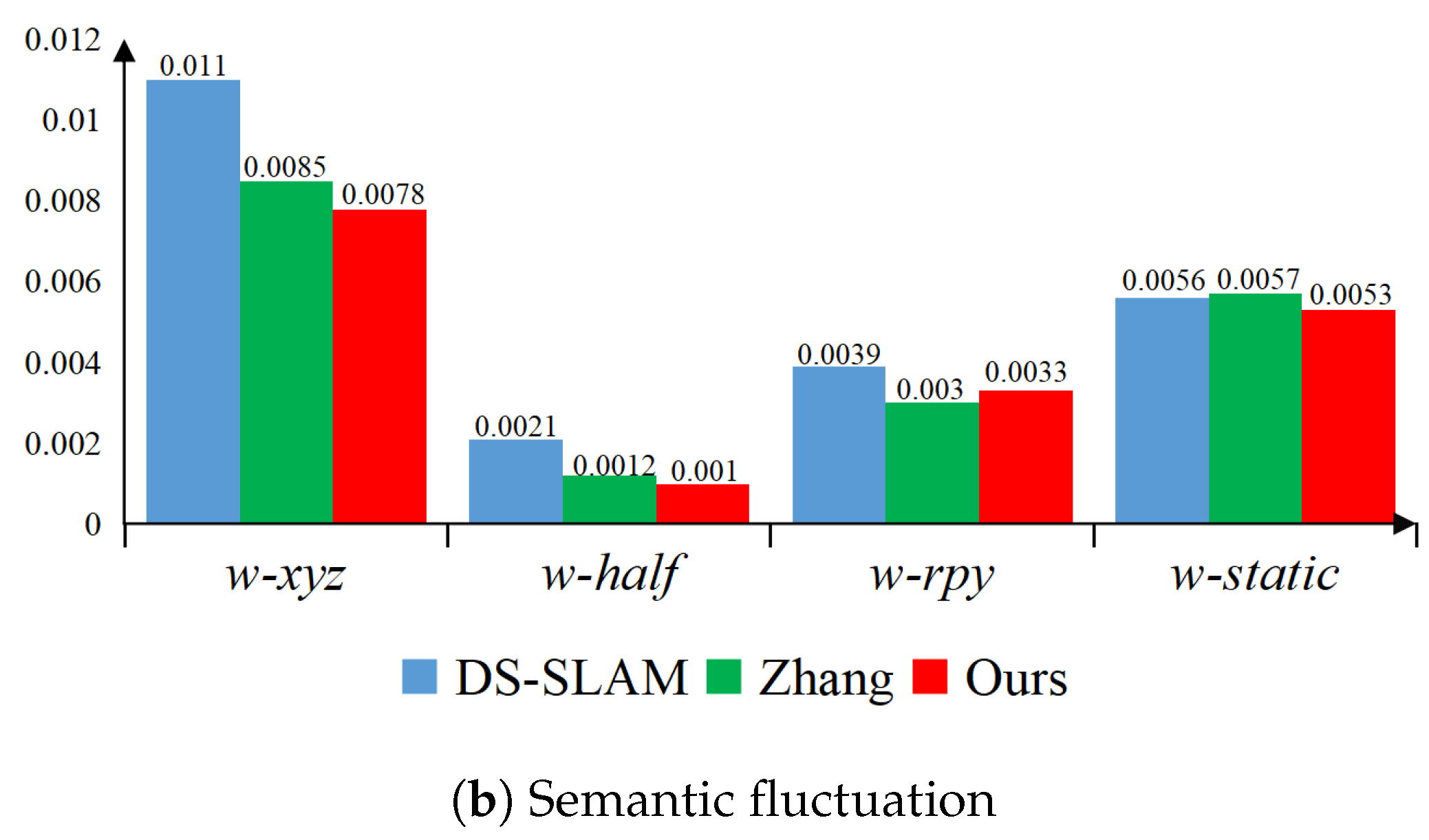
| w-static | 0.3340 | 0.1444 | 0.0091 | 0.0041 | 0.0087 | 0.0044 | 0.0078 | 0.0033 |
| Algorithm | ORB- SLAM2 | Dyna- SLAM | DO- SLAM | YOLO- SLAM | Ours |
|---|---|---|---|---|---|
| Hardware platform | — | Nvidia Tesla M40 GPU | Inter Core i5-4288U | Intel Core i5-4288U CPU | Nvidia Geforce RTX 3050 GPU |
| Network | — | Mask R-CNN | YOLOv5 | YOLOv3 | YOLOv8-seg |
| Segmentation /Detection time (ms) | — | 195 | 81.44 | 696.09 | 25.28 |
| Tracking time (/ms) | 22.8602 | >300 | 118.23 | 651.53 | 26.7219 |
| Types of Scenes | Algorithm | Number of Closed-Loop | TP | FP | FN | Precision | Recall |
|---|---|---|---|---|---|---|---|
| Dynamic interference | BoW | 8 | 6 | 0 | 2 | 100% | 62.50% |
| BoW+GE | 8 | 8 | 0 | 0 | 100% | 100% | |
| Structural changes | BoW | 8 | 7 | 0 | 1 | 100% | 87.50% |
| BoW+GE | 8 | 8 | 0 | 0 | 100% | 100% |
Disclaimer/Publisher’s Note: The statements, opinions and data contained in all publications are solely those of the individual author(s) and contributor(s) and not of MDPI and/or the editor(s). MDPI and/or the editor(s) disclaim responsibility for any injury to people or property resulting from any ideas, methods, instructions or products referred to in the content. |
© 2025 by the authors. Licensee MDPI, Basel, Switzerland. This article is an open access article distributed under the terms and conditions of the Creative Commons Attribution (CC BY) license (https://creativecommons.org/licenses/by/4.0/).
Share and Cite
Wang, D.; Luo, J. Approach to Semantic Visual SLAM for Bionic Robots Based on Loop Closure Detection with Combinatorial Graph Entropy in Complex Dynamic Scenes. Biomimetics 2025, 10, 446. https://doi.org/10.3390/biomimetics10070446
Wang D, Luo J. Approach to Semantic Visual SLAM for Bionic Robots Based on Loop Closure Detection with Combinatorial Graph Entropy in Complex Dynamic Scenes. Biomimetics. 2025; 10(7):446. https://doi.org/10.3390/biomimetics10070446
Chicago/Turabian StyleWang, Dazheng, and Jingwen Luo. 2025. "Approach to Semantic Visual SLAM for Bionic Robots Based on Loop Closure Detection with Combinatorial Graph Entropy in Complex Dynamic Scenes" Biomimetics 10, no. 7: 446. https://doi.org/10.3390/biomimetics10070446
APA StyleWang, D., & Luo, J. (2025). Approach to Semantic Visual SLAM for Bionic Robots Based on Loop Closure Detection with Combinatorial Graph Entropy in Complex Dynamic Scenes. Biomimetics, 10(7), 446. https://doi.org/10.3390/biomimetics10070446