

A Novel Improved Dung Beetle Optimization Algorithm for Collaborative 3D Path Planning of UAVs

Abstract

1. Introduction
- An Environment-aware Chaotic Force–field Dung Beetle Optimizer (ECFDBO) is proposed by us, which augments the original Dung Beetle Optimizer (DBO) with three novel improvement strategies: chaotic perturbation mixed nonlinear contraction, environment-aware boundary handling, and dynamic attraction–repulsion field mutation. It ensures stable performance in high-dimensional search spaces.
- ECFDBO was subjected to multi-perspective, multi-run experiments by us on the CEC2017 (Dim = 30, 50, and 100) suite to assess its robustness and effectiveness. Wilcoxon and Friedman’s tests demonstrate that ECFDBO’s performance differences among seven state-of-the-art metaheuristics are statistically significant.
- We formulate the multi-UAV coordination task as a multi-constrained optimization problem with several key constraints based on the application of UAV tasks in remote sensing. Additionally, we apply the cooperative path-planning model to four distinct environments to validate its simulated effectiveness.
2. Preliminary Knowledge
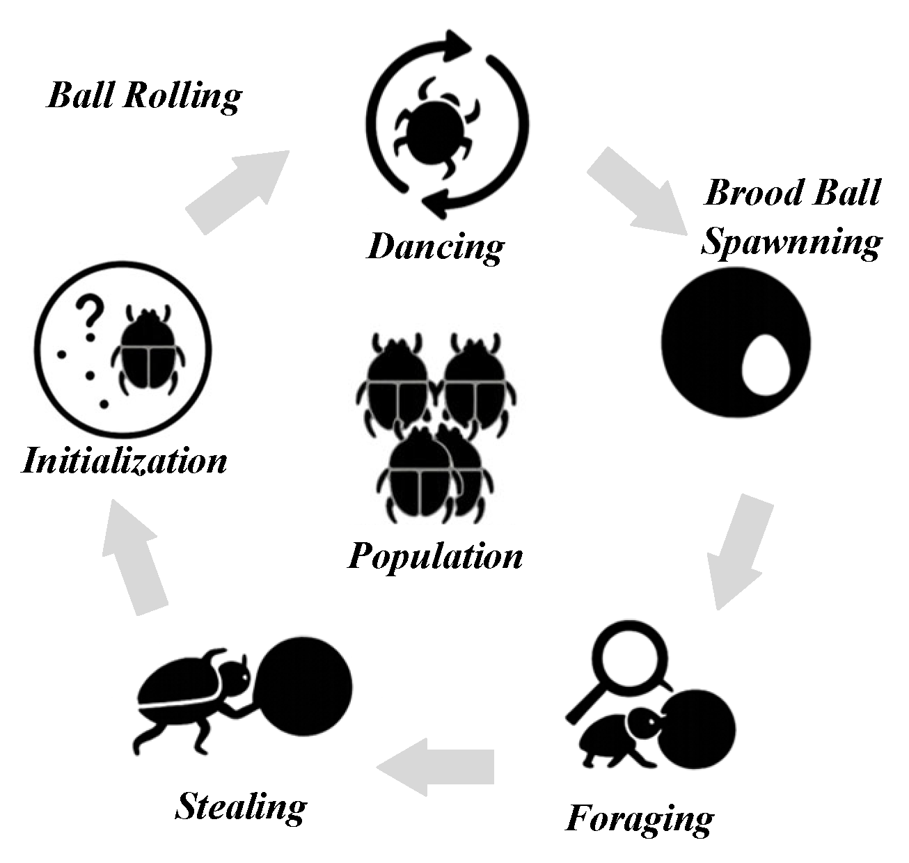
2.1. Population Initialization
2.2. Rolling Stage
2.2.1. Obstacle-Free Mode
2.2.2. Obstacle Mode
2.3. Reproduction Behavior
2.4. Foraging Behavior
2.5. Stealing Behavior
| Algorithm 1: DBO (Dung Beetle Optimizer) |
| Input: population size: N; problem dimension: d; search boundary: [lb, ub]; maximum number of iterations: Tmax; fitness function: f(x) Output: Optimal position: Xbest |
| 1: Initialize Xi ∼ Uniform(lb, ub) for i = 1…N ←Calculated using Equation (1) 2: Evaluate fi = f(Xi), set Xbest = argmin fi, Xworst = argmax fi 3: for t = 1 to Tmax do 4: p = ⌊0.2·N⌋ 5: // Rolling stage 6: for i = 1 to p do 7: if rand() < 0.9 then 8: Xi ←Calculated using Equation (2) 9: else 10: Xi ←Calculated using Equation (3) 11: end if 12: end for 13: // Reproduction stage 14: R = 1 − t/Tmax 15: [Lb*, Ub*] ←Calculated using Equation (4) 16: for i = p + 1 to p + m do 17: Xi ←Calculated using Equation (5) 18: end for 19: // Foraging stage 20: for i = p + m+1 to p + m+q do 21: Xi ←Calculated using Equation (6) 22: end for 23: // Stealing stage 24: for i = p + m+q + 1 to N do 25: Xi ←Calculated using Equation (7) 26: end for 27: // Boundary check 28: for i = 1 to N do 29: Xi = clip(Xi, lb, ub) 30: end for 31: Evaluate all fi, update Xbest, Xworst 32: end for 33: return Xbest |
3. Proposed Algorithm
3.1. Chaotic Perturbation Mixed Nonlinear Contraction Mechanisms
3.2. Environment-Aware Boundary-Handling Strategy
3.3. Dynamic Attraction–Repulsion Force-Field Mutation Strategy
| Algorithm 2: ECFDBO (Environment-aware Chaotic Force-field Dung Beetle Optimizer) |
| Input: population size: N; problem dimension: d; search boundary: [lb, ub]; maximum number of iterations: Tmax; fitness function: f(x) Output: Optimal position: Xbest |
| 1: Initialize {Xi}₁ⁿ ∼ Uniform (lb, ub) 2: Evaluate fi, set Xbest 3: for t = 1…Tmax do 4: // Construct the set of suboptimal solutions Q 5: Sort {Xi} by fitness, let Q ← best K = max (3, ⌊0.1·N⌋) 6: for each i = 1…N do 7: Compute 8: Fi ← Fg − Fr← Calculated using Equation (14) 9: if rand () < pm then 10: η ←Calculated using Equation (15) 11: Xi ←Attraction–Repulsion Mutation 12: else 13: // Chaos Steps Update 14: Xi ← Calculated using Equation (9) 15: end if 16: Xi ← SmartReflect(Xi, lb, ub, ε) ← Calculated using Equation (12) 17: end for 18: {Xi}← DBO_ Stage({Xi}) // Rolling, Reproduction, Foraging, Stealing 19: Evaluate all fi, update Xbest 20: end for 21: return Xbest |
4. Complexity Analysis
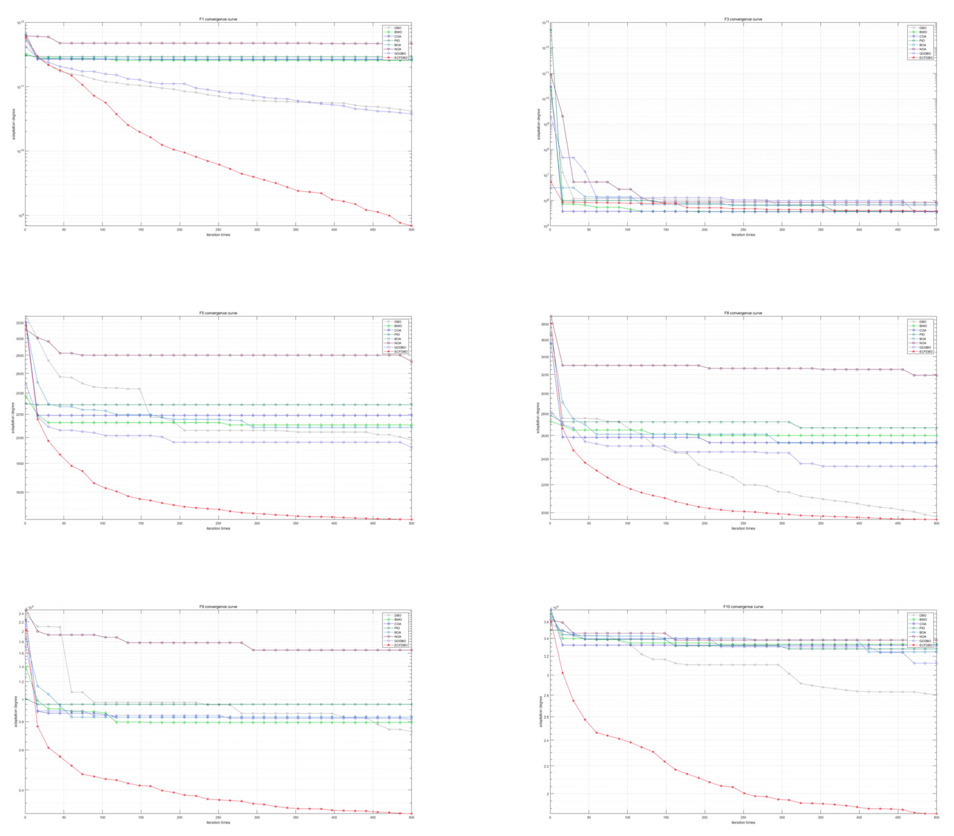
5. CEC2017 Test
5.1. CEC2017 Introduction
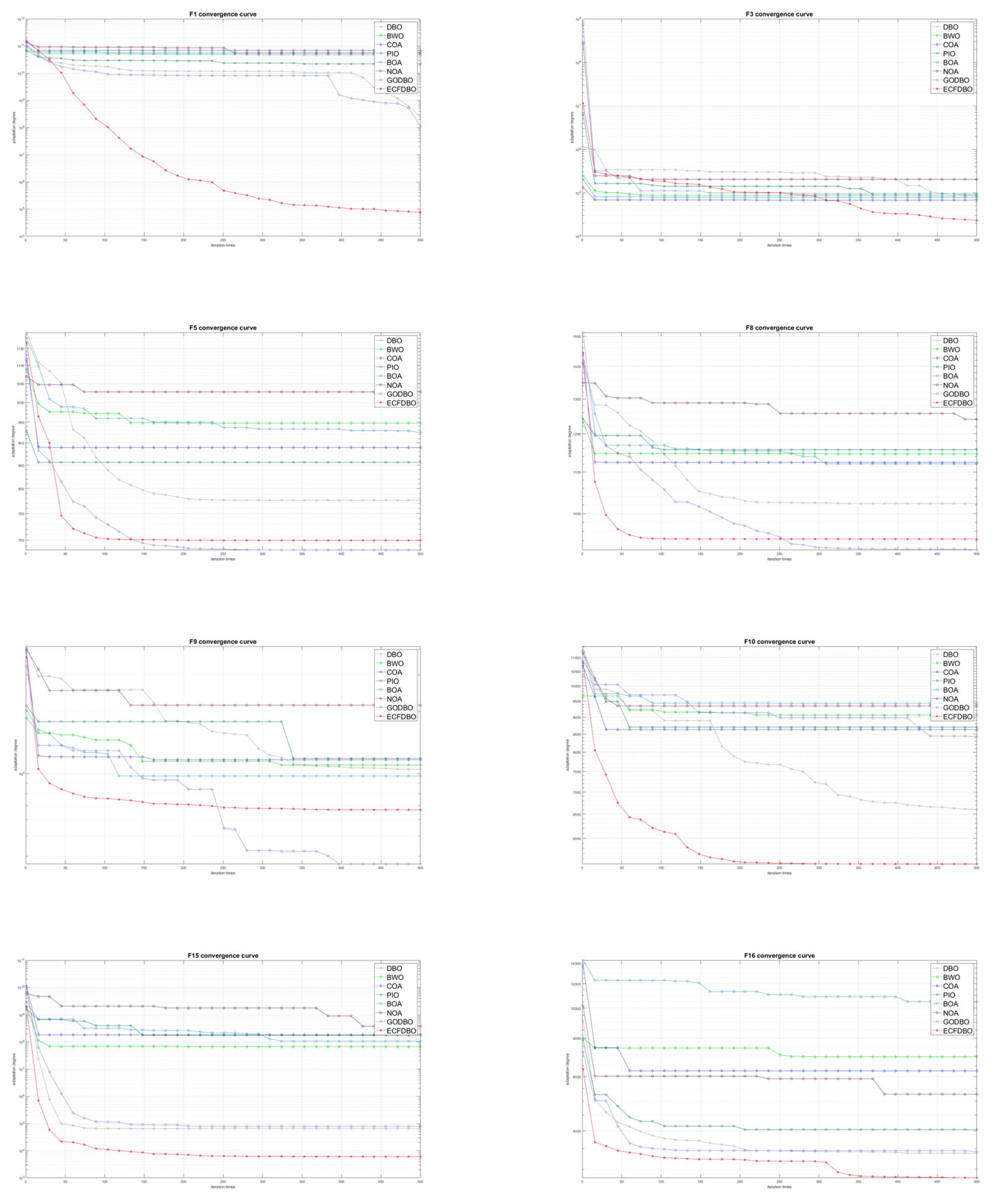
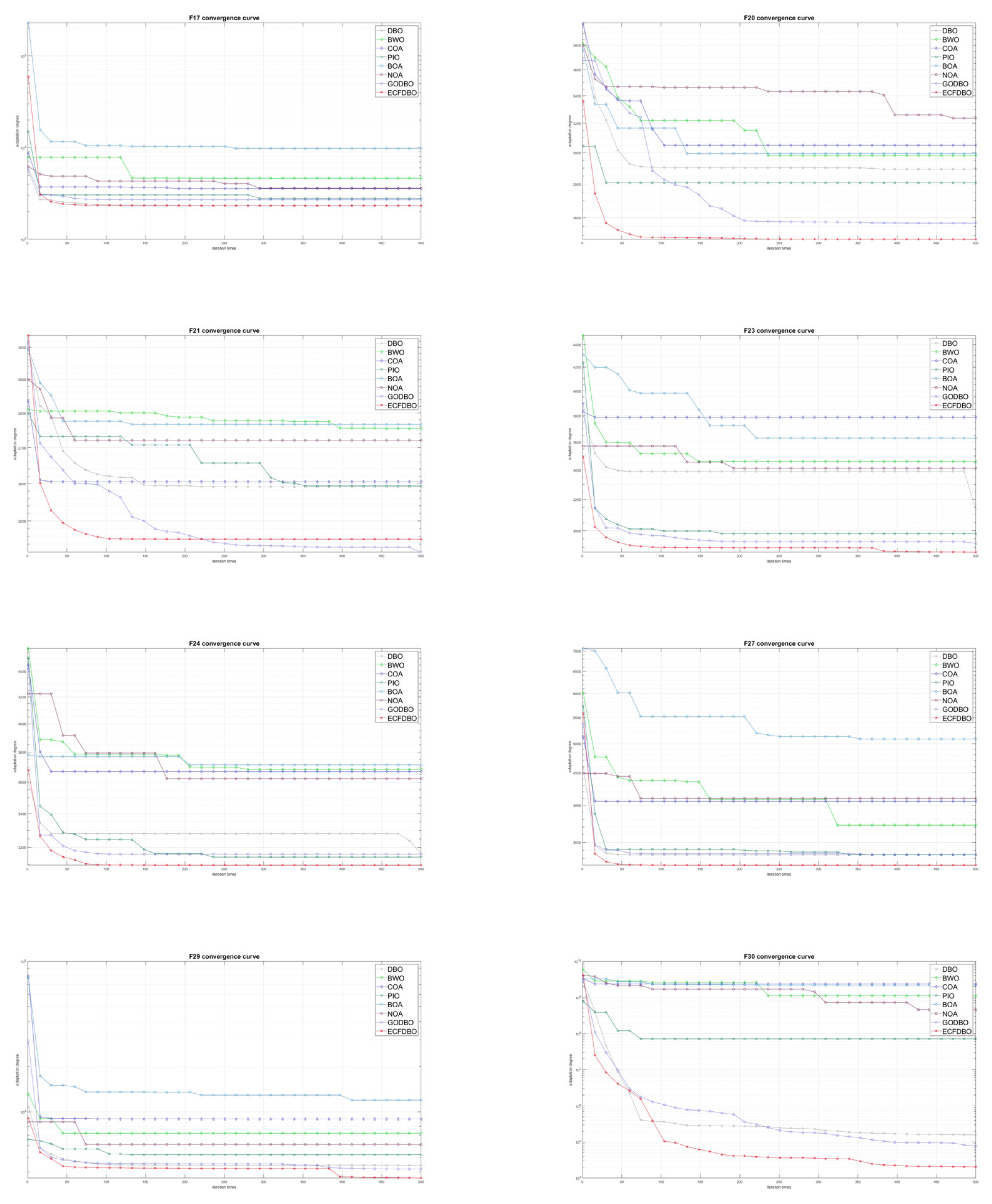
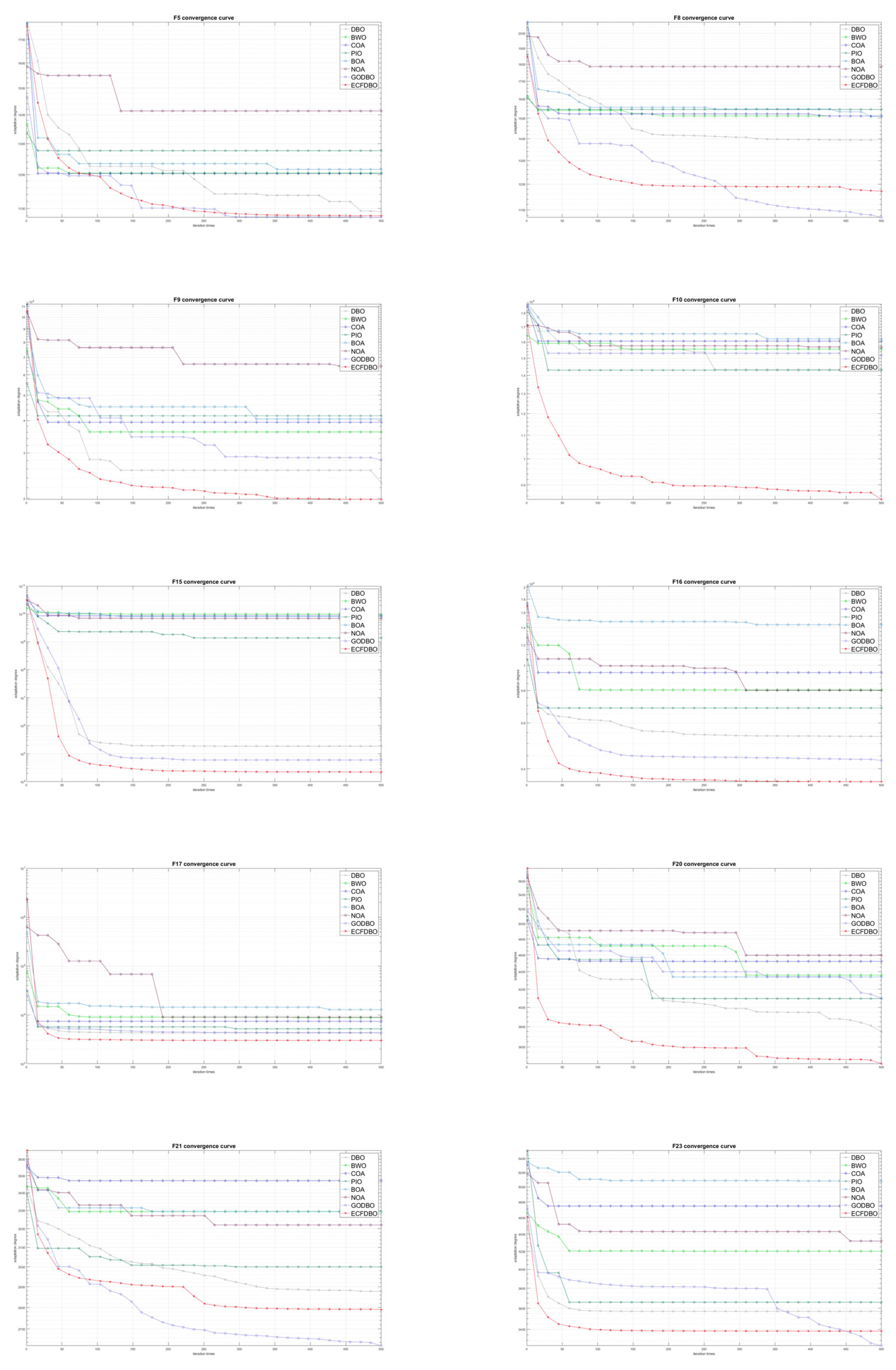
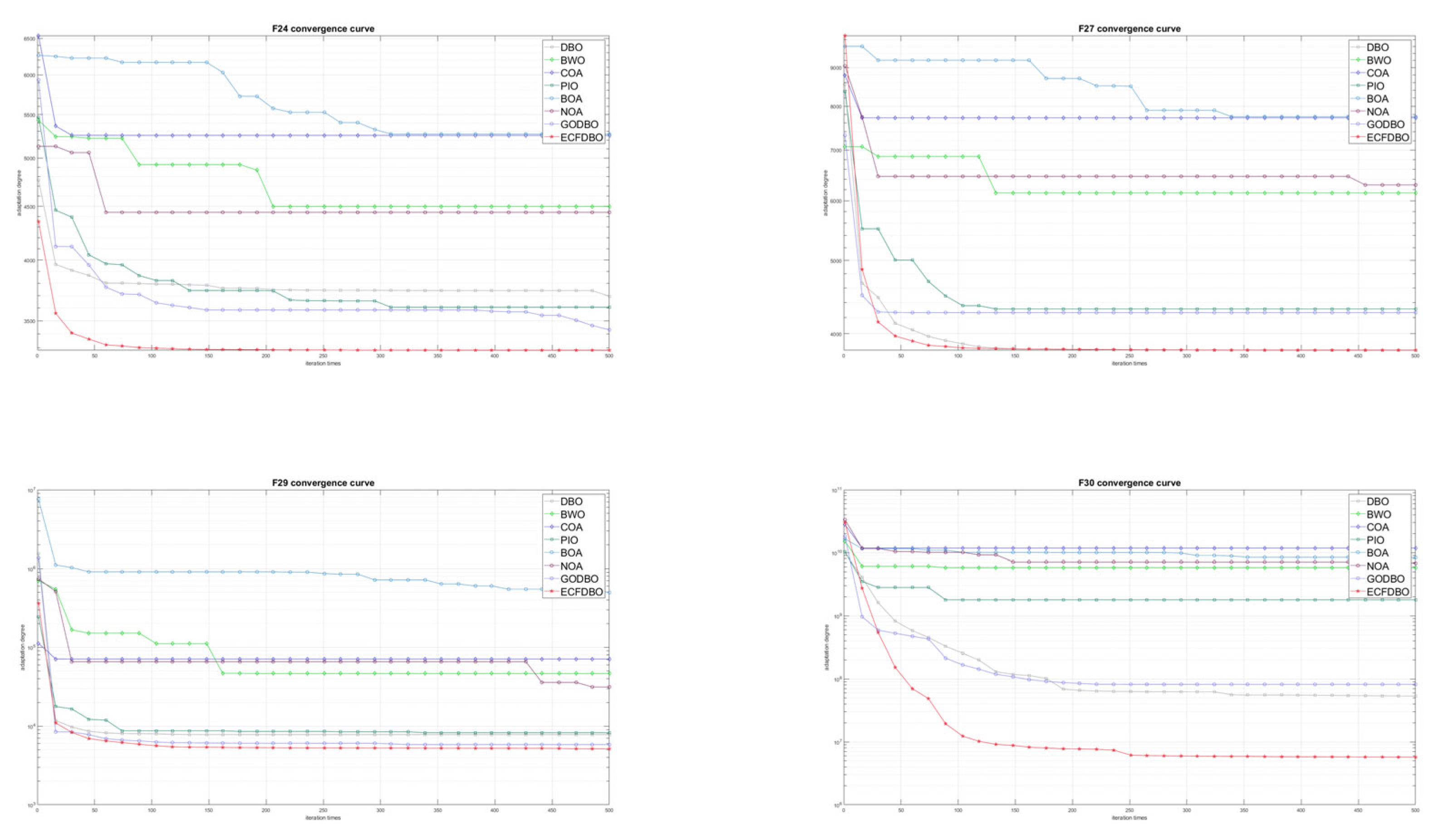
5.2. Comparison with Mainstream Optimization Algorithms
5.3. Wilcoxon and Friedman Statistical Tests
5.4. Contribution of the Improvement Strategies
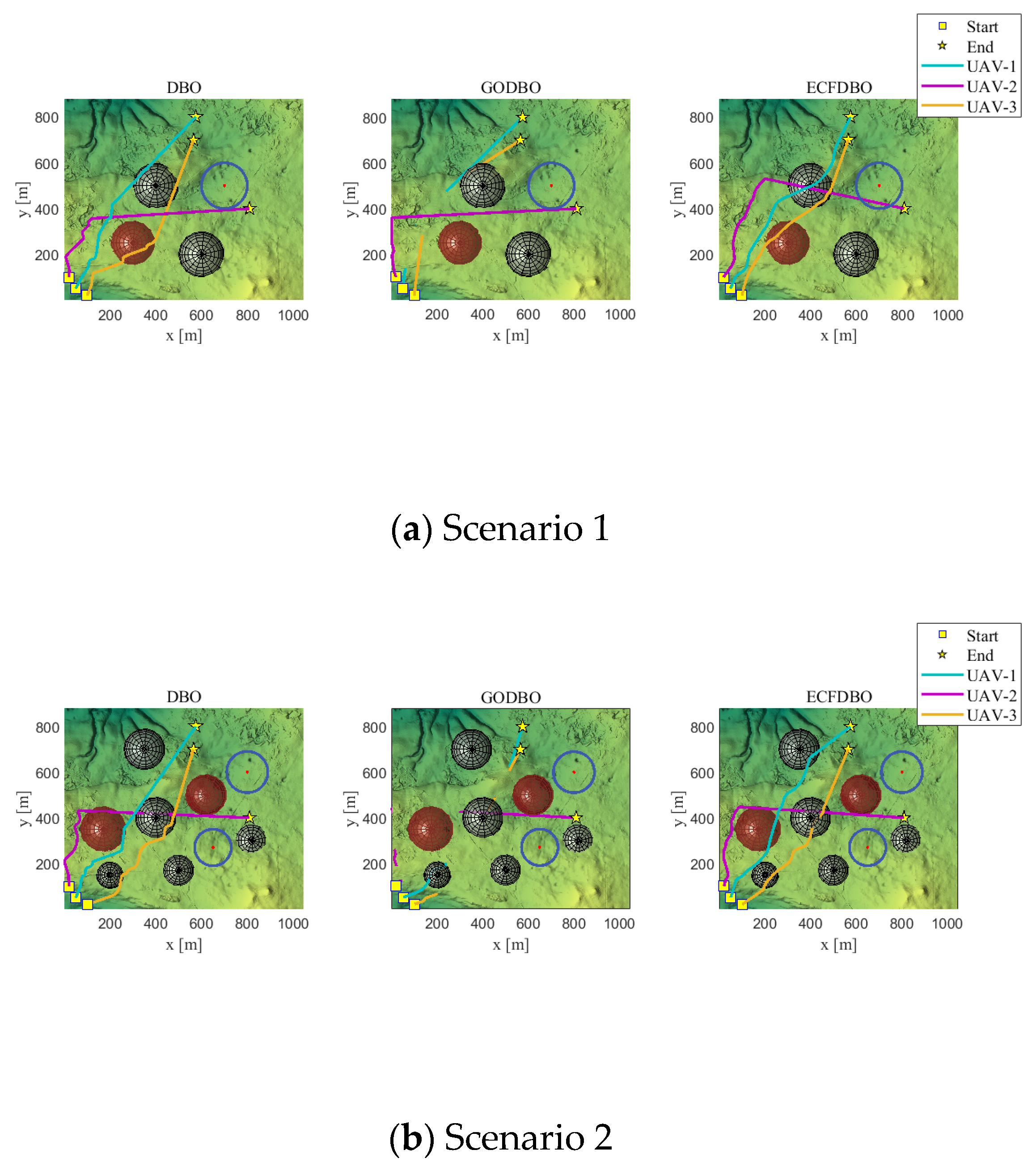
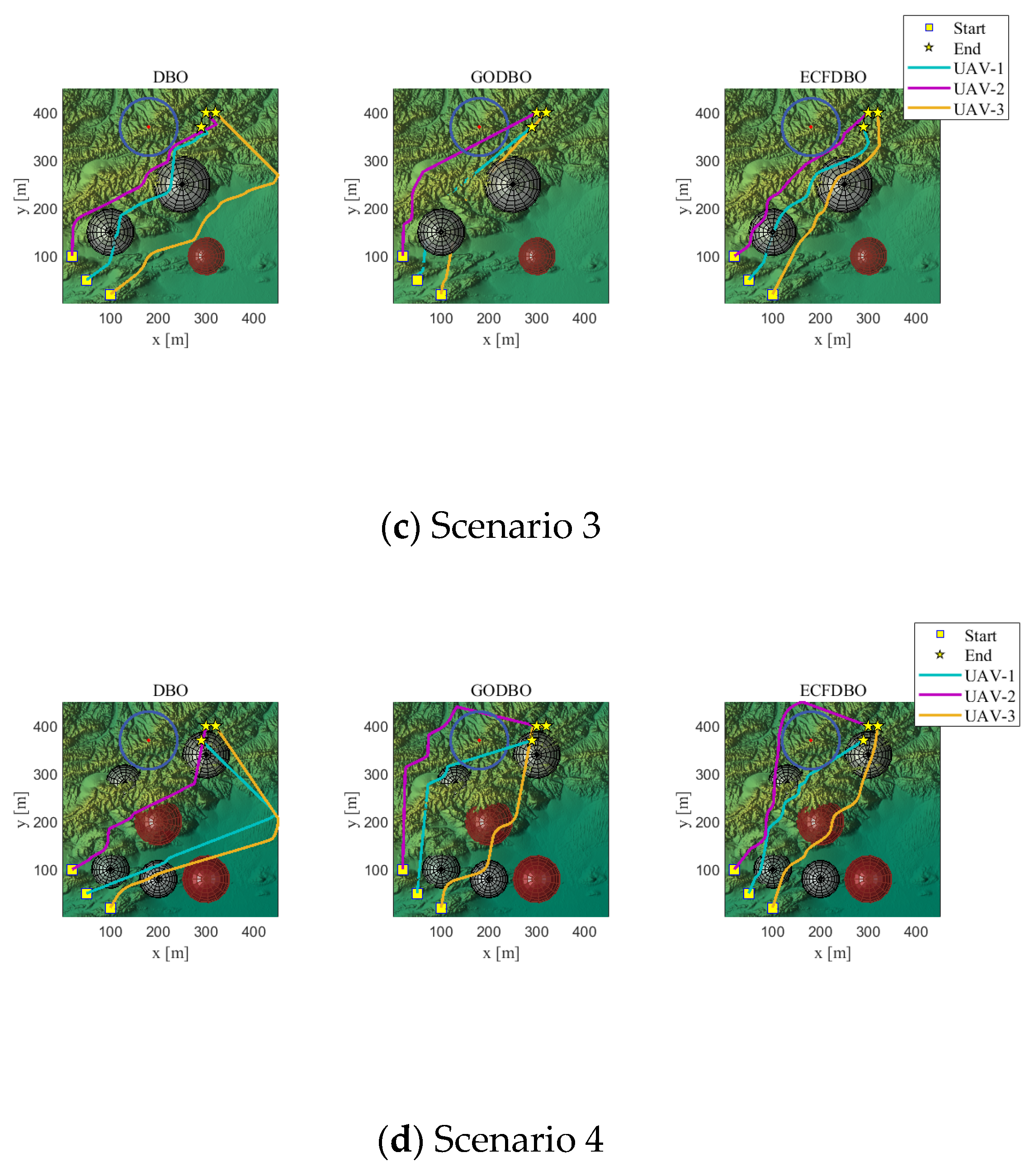
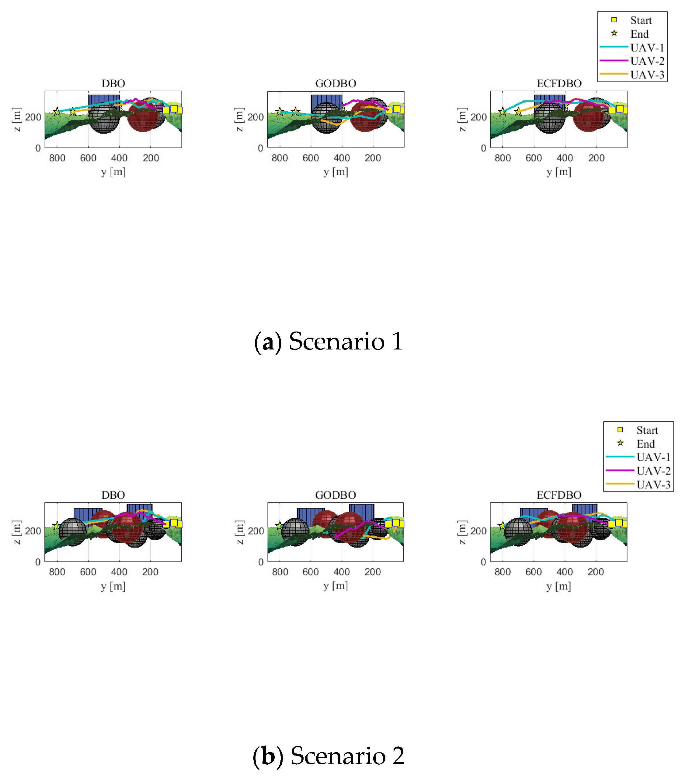
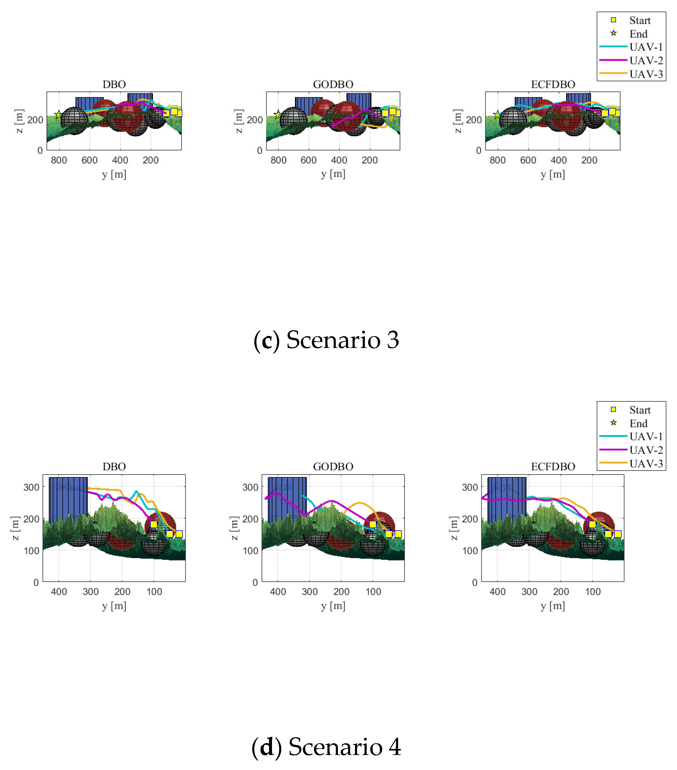
6. Collaborative 3D Path Planning Simulation
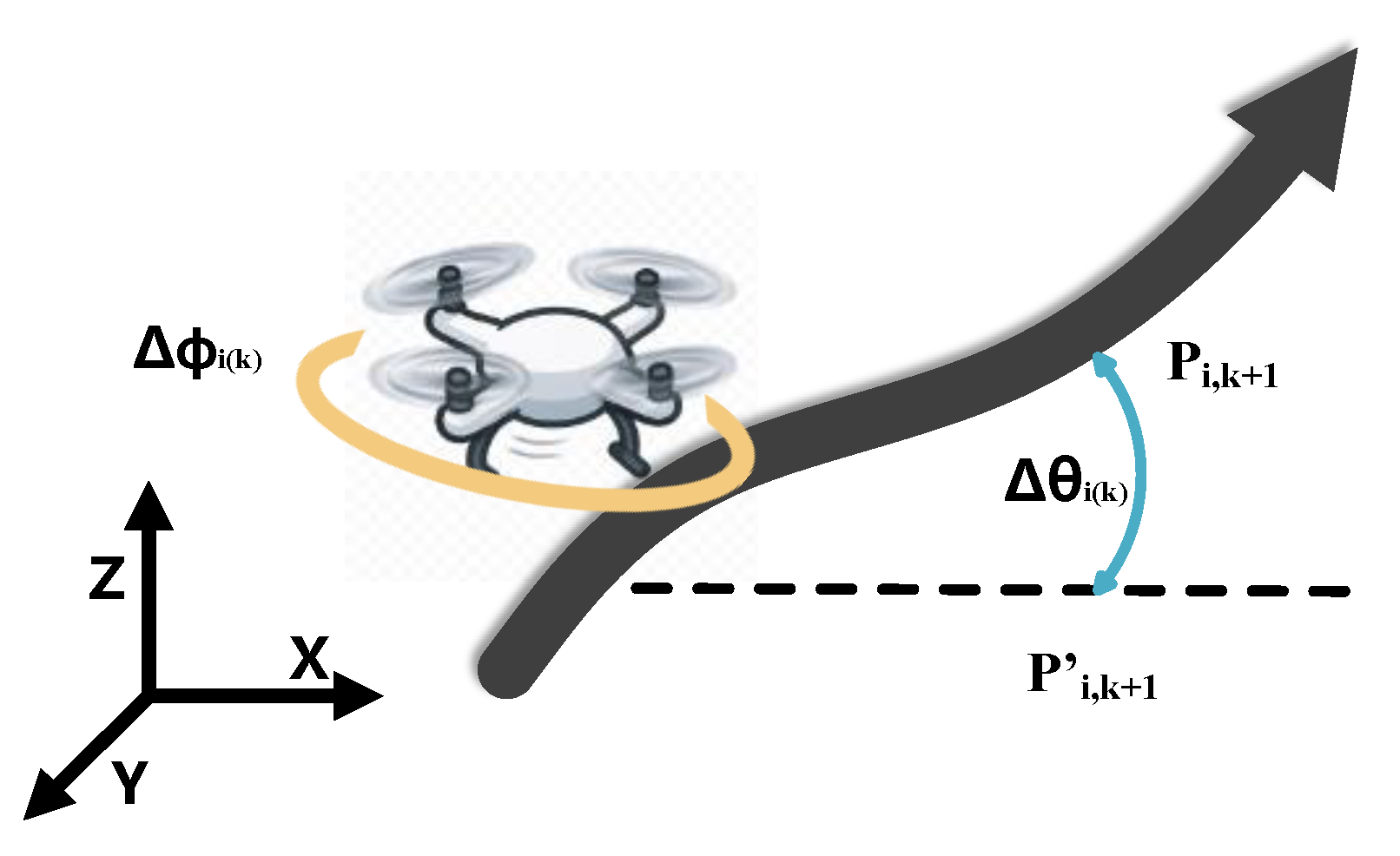
6.1. Problem Statement
6.1.1. Flight Path Distance
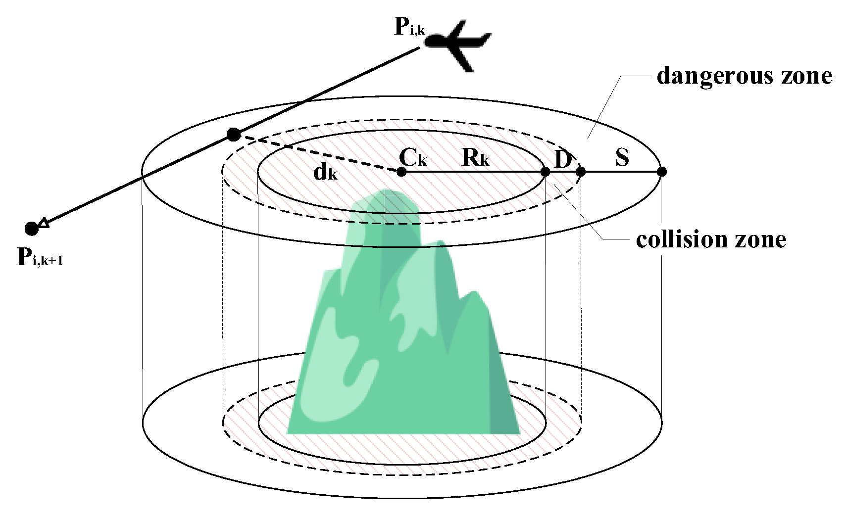
6.1.2. Security and Threat Constraints
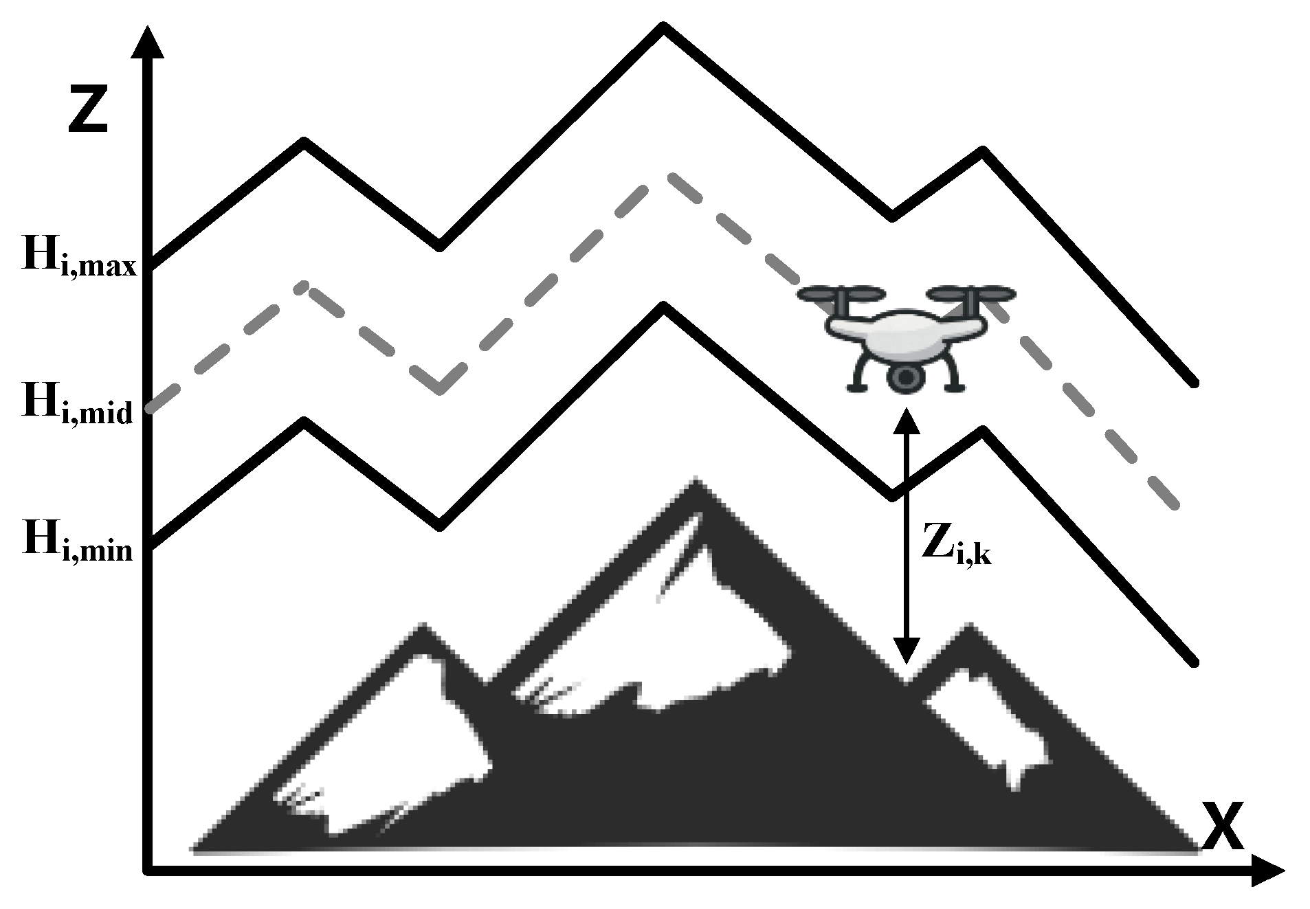
6.1.3. Cost of Flight Altitude
6.1.4. Path Smoothness
6.1.5. Time Synchronization Constraint
6.1.6. Space Collision Costs
6.1.7. Minimum Path Segment Interval Constraint
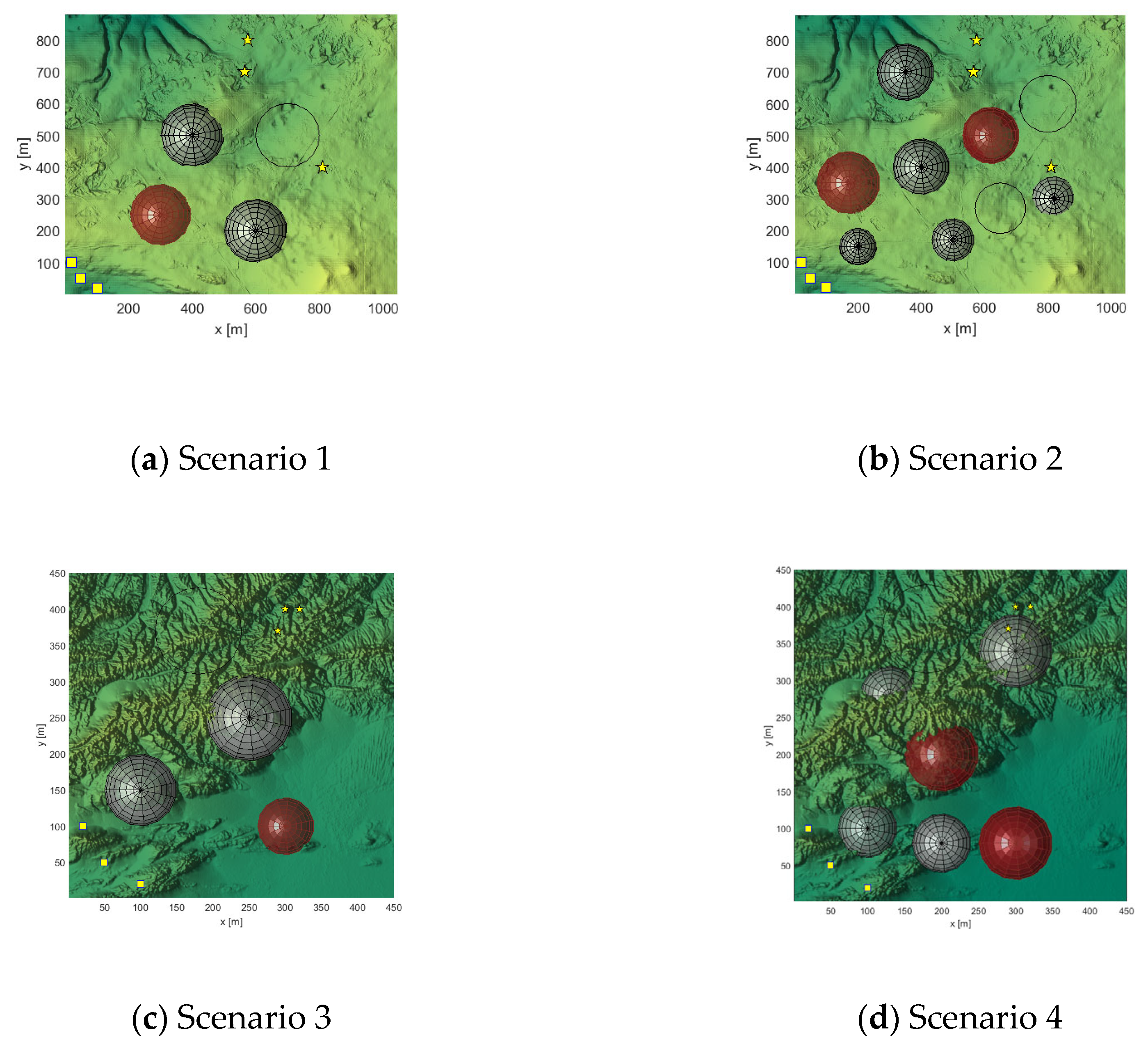
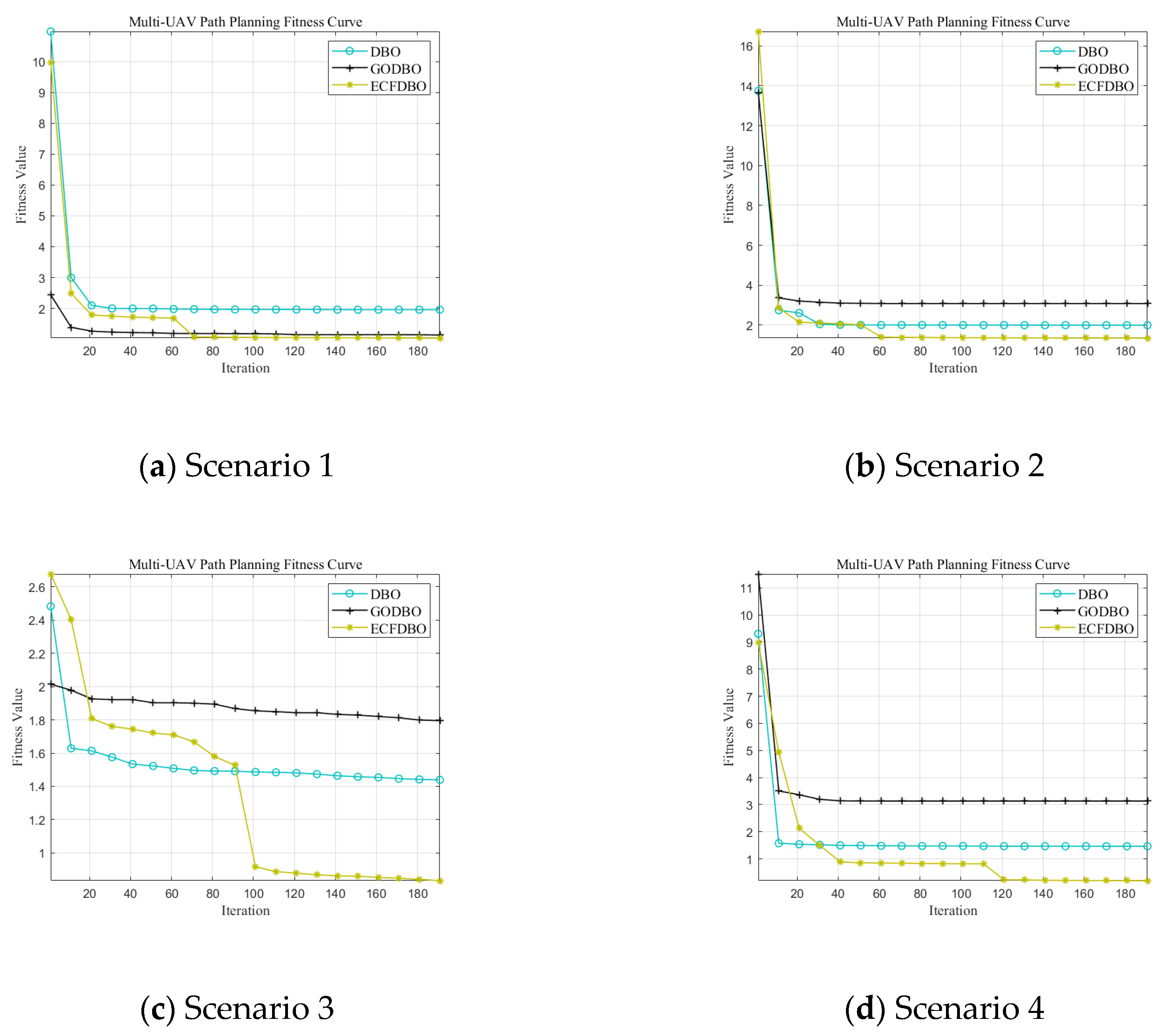
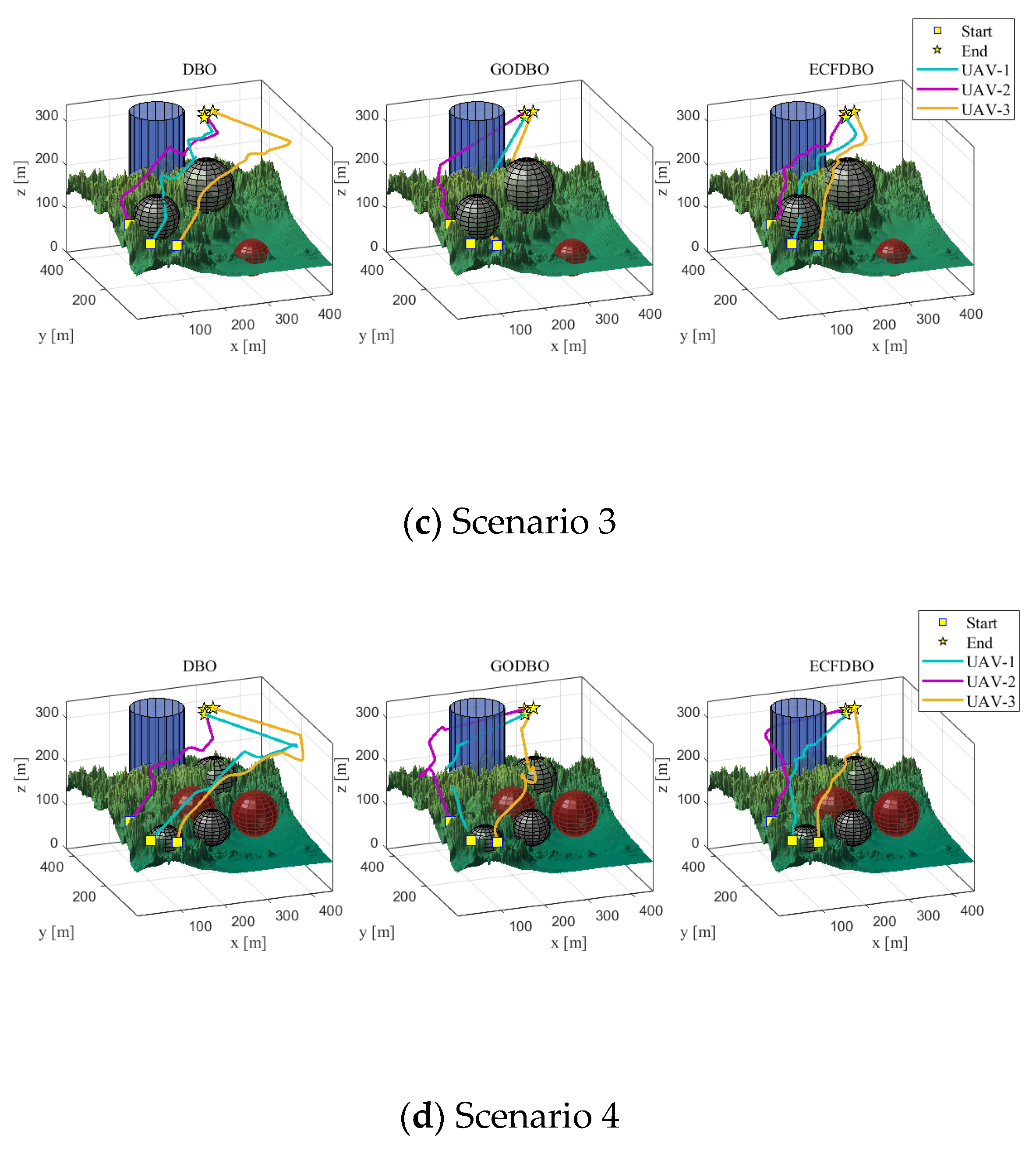
6.2. Simulation Experiment
7. Conclusions
Author Contributions
Funding
Data Availability Statement
Conflicts of Interest
Appendix A


References
- Ndlovu, H.S.; Odindi, J.; Sibanda, M.; Mutanga, O. A systematic review on the application of UAV-based thermal remote sensing for assessing and monitoring crop water status in crop farming systems. Int. J. Remote Sens. 2024, 45, 4923–4960. [Google Scholar] [CrossRef]
- Yang, Z.; Yu, X.; Dedman, S.; Rosso, M.; Zhu, J.; Yang, J.; Xia, Y.; Tian, Y.; Zhang, G.; Wang, J. UAV remote sensing applications in marine monitoring: Knowledge visualization and review. Sci. Total Environ. 2022, 838, 155939. [Google Scholar] [CrossRef] [PubMed]
- Guan, S.; Zhu, Z.; Wang, G. A review on UAV-based remote sensing technologies for construction and civil applications. Drones 2022, 6, 117. [Google Scholar] [CrossRef]
- Debnath, D.; Hawary, A.F.; Ramdan, M.I.; Alvarez, F.V.; Gonzalez, F. QuickNav: An effective collision avoidance and path-planning algorithm for UAS. Drones 2023, 7, 678. [Google Scholar] [CrossRef]
- Meng, Q.; Qu, Q.; Chen, K.; Yi, T. Multi-UAV Path Planning Based on Cooperative Co-Evolutionary Algorithms with Adaptive Decision Variable Selection. Drones 2024, 8, 435. [Google Scholar] [CrossRef]
- Maboudi, M.; Homaei, M.R.; Song, S.; Malihi, S.; Saadatseresht, M.; Gerke, M. A review on viewpoints and path planning for UAV-based 3-D reconstruction. IEEE J. Sel. Top. Appl. Earth Obs. Remote Sens. 2023, 16, 5026–5048. [Google Scholar] [CrossRef]
- Zhang, Z.; Zhu, L. A review on unmanned aerial vehicle remote sensing: Platforms, sensors, data processing methods, and applications. Drones 2023, 7, 398. [Google Scholar] [CrossRef]
- Nex, F.; Remondino, F. UAV for 3D mapping applications: A review. Appl. Geomat. 2014, 6, 1–15. [Google Scholar] [CrossRef]
- Mazaheri, H.; Goli, S.; Nourollah, A. A Survey of 3D Space Path-Planning Methods and Algorithms. ACM Comput. Surv. 2024, 57, 1–32. [Google Scholar] [CrossRef]
- Dechter, R.; Pearl, J. Generalized best-first search strategies and the optimality of A. J. ACM 1985, 32, 505–536. [Google Scholar] [CrossRef]
- Hart, P.E.; Nilsson, N.J.; Raphael, B. A formal basis for the heuristic determination of minimum cost paths. IEEE Trans. Syst. Sci. Cybern. 1968, 4, 100–107. [Google Scholar] [CrossRef]
- Mandloi, D.; Arya, R.; Verma, A.K. Unmanned aerial vehicle path planning based on A* algorithm and its variants in 3d environment. Int. J. Syst. Assur. Eng. Manag. 2021, 12, 990–1000. [Google Scholar] [CrossRef]
- Bai, X.; Jiang, H.; Cui, J.; Lu, K.; Chen, P.; Zhang, M. UAV path planning based on improved A∗ and DWA algorithms. Int. J. Aerosp. Eng. 2021, 2021, 4511252. [Google Scholar] [CrossRef]
- Chen, J.; Li, M.; Yuan, Z.; Gu, Q. An improved A* algorithm for UAV path planning problems. In Proceedings of the IEEE 4th Information Technology, Networking, Electronic and Automation Control Conference (ITNEC), Chongqing, China, 12–14 June 2020; Volume 1, pp. 958–962. [Google Scholar]
- Sun, S.; Wang, H.; Xu, Y.; Wang, T.; Liu, R.; Chen, W. A Fusion Approach for UAV Onboard Flight Path Management and Decision Making Based on the Combination of Enhanced A* Algorithm and Quadratic Programming. Drones 2024, 8, 254. [Google Scholar] [CrossRef]
- Huang, C. A Novel Three-Dimensional Path Planning Method for Fixed-Wing UAV Using Improved Particle Swarm Optimization Algorithm. Int. J. Aerosp. Eng. 2021, 2021, 7667173. [Google Scholar] [CrossRef]
- Heidari, H.; Saska, M. Collision-free path planning of multi-rotor UAVs in a wind condition based on modified potential field. Mech. Mach. Theory 2021, 156, 104140. [Google Scholar] [CrossRef]
- Di, B.; Zhou, R.; Duan, H. Potential field based receding horizon motion planning for centrality-aware multiple UAV cooperative surveillance. Aerosp. Sci. Technol. 2015, 46, 386–397. [Google Scholar] [CrossRef]
- Noreen, I.; Khan, A.; Habib, Z. Optimal path planning using RRT* based approaches: A survey and future directions. Int. J. Adv. Comput. Sci. Appl. 2016, 7, 97–107. [Google Scholar] [CrossRef]
- Guo, Y.; Liu, X.; Yang, Y.; Zhang, W. FC-RRT*: An improved path planning algorithm for UAV in 3D complex environment. ISPRS Int. J. Geo. Inf. 2022, 11, 112. [Google Scholar] [CrossRef]
- Phung, M.D.; Ha, Q.P. Safety-enhanced UAV path planning with spherical vector-based particle swarm optimization. Appl. Soft Comput. 2021, 107, 107376. [Google Scholar] [CrossRef]
- Pehlivanoglu, Y.V.; Pehlivanoglu, P. An enhanced genetic algorithm for path planning of autonomous UAV in target coverage problems. Appl. Soft Comput. 2021, 112, 107796. [Google Scholar] [CrossRef]
- Roberge, V.; Tarbouchi, M.; Labonté, G. Comparison of parallel genetic algorithm and particle swarm optimization for real-time UAV path planning. IEEE Trans. Ind. Inform. 2012, 9, 132–141. [Google Scholar] [CrossRef]
- Kennedy, J. Handbook of Nature-Inspired and Innovative Computing: Integrating Classical Models with Emerging Technologies; Springer: Boston, MA, USA, 2006; pp. 187–219. [Google Scholar]
- Fu, Y.; Ding, M.; Zhou, C. Phase angle-encoded and quantum-behaved particle swarm optimization applied to three-dimensional route planning for UAV. IEEE Trans. Syst. Man Cybern. Part A Syst. Hum. 2011, 42, 511–526. [Google Scholar] [CrossRef]
- Wei-Min, Z.; Shao-Jun, L.; Feng, Q. θ-PSO: A new strategy of particle swarm optimization. J. Zhejiang Univ. Sci. A 2008, 9, 786–790. [Google Scholar] [CrossRef]
- Hoang, V.T.; Phung, M.D.; Dinh, T.H.; Ha, Q.P. Angle-encoded swarm optimization for uav formation path planning. In Proceedings of the IEEE/RSJ International Conference on Intelligent Robots and Systems (IROS), Madrid, Spain, 1–5 October 2018; pp. 5239–5244. [Google Scholar]
- Sun, J.; Fang, W.; Wu, X.; Palade, V.; Xu, W. Quantum-behaved particle swarm optimization: Analysis of individual particle behavior and parameter selection. Evol. Comput. 2012, 20, 349–393. [Google Scholar] [CrossRef]
- Phung, M.D.; Quach, C.H.; Dinh, T.H.; Ha, Q. Enhanced discrete particle swarm optimization path planning for UAV vision-based surface inspection. Autom. Constr. 2017, 81, 25–33. [Google Scholar] [CrossRef]
- Onwubolu, G.C.; Babu, B.V.; Clerc, M. Discrete particle swarm optimization, illustrated by the traveling salesman problem. New Optim. Tech. Eng. 2004, 47, 219–239. [Google Scholar]
- Yu, X.; Jiang, N.; Wang, X.; Li, M. A hybrid algorithm based on grey wolf optimizer and differential evolution for UAV path planning. Expert Syst. Appl. 2023, 215, 119327. [Google Scholar] [CrossRef]
- Yu, X.; Chen, W.N.; Gu, T.; Yuan, H.; Zhang, H.; Zhang, J. ACO-A*: Ant colony optimization plus A* for 3-D traveling in environments with dense obstacles. IEEE Trans. Evol. Comput. 2018, 23, 617–631. [Google Scholar] [CrossRef]
- Xu, C.; Duan, H.; Liu, F. Chaotic artificial bee colony approach to Uninhabited Combat Air Vehicle (UCAV) path planning. Aerosp. Sci. Technol. 2010, 14, 535–541. [Google Scholar] [CrossRef]
- Debnath, D.; Vanegas, F.; Sandino, J.; Hawary, A.F.; Gonzalez, F. A Review of UAV Path-Planning Algorithms and Obstacle Avoidance Methods for Remote Sensing Applications. Remote Sens. 2024, 16, 4019. [Google Scholar] [CrossRef]
- Dehghani, M.; Montazeri, Z.; Trojovská, E.; Trojovský, P. Coati Optimization Algorithm: A new bio-inspired metaheuristic algorithm for solving optimization problems. Knowl. Based Syst. 2023, 259, 110011. [Google Scholar] [CrossRef]
- Arora, S.; Singh, S. Butterfly optimization algorithm: A novel approach for global optimization. Soft Comput. 2019, 23, 715–734. [Google Scholar] [CrossRef]
- Zhong, C.; Li, G.; Meng, Z. Beluga whale optimization: A novel nature-inspired metaheuristic algorithm. Knowl. Based Syst. 2022, 251, 109215. [Google Scholar] [CrossRef]
- Duan, H.; Qiao, P. Pigeon-inspired optimization: A new swarm intelligence optimizer for air robot path planning. Int. J. Intell. Comput. Cybern. 2014, 7, 24–37. [Google Scholar] [CrossRef]
- Abdel-Basset, M.; Mohamed, R.; Jameel, M.; Abouhawwash, M. Nutcracker optimizer: A novel nature-inspired metaheuristic algorithm for global optimization and engineering design problems. Knowl. Based Syst. 2023, 262, 110248. [Google Scholar] [CrossRef]
- Liu, B.; Cai, Y.; Li, D.; Lin, K.; Xu, G. A Hybrid ARO Algorithm and Key Point Retention Strategy Trajectory Optimization for UAV Path Planning. Drones 2024, 8, 644. [Google Scholar] [CrossRef]
- Xue, J.; Shen, B. Dung beetle optimizer: A new meta-heuristic algorithm for global optimization. J. Supercomput. 2023, 79, 7305–7336. [Google Scholar] [CrossRef]
- Shen, Q.; Zhang, D.; Xie, M.; He, Q. Multi-strategy enhanced dung beetle optimizer and its application in three-dimensional UAV path planning. Symmetry 2023, 15, 1432. [Google Scholar] [CrossRef]
- Tang, X.; He, Z.; Jia, C. Multi-strategy cooperative enhancement dung beetle optimizer and its application in obstacle avoidance navigation. Sci. Rep. 2024, 14, 28041. [Google Scholar] [CrossRef]
- Zilong, W.; Peng, S. A multi-strategy dung beetle optimization algorithm for optimizing constrained engineering problems. IEEE Access 2023, 11, 98805–98817. [Google Scholar] [CrossRef]
- Hu, W.; Zhang, Q.; Ye, S. An enhanced dung beetle optimizer with multiple strategies for robot path planning. Sci. Rep. 2025, 15, 4655. [Google Scholar] [CrossRef] [PubMed]
- Zhang, R.; Chen, X.; Li, M. Multi-UAV cooperative task assignment based on multi-strategy improved DBO. Clust. Comput. 2025, 28, 195. [Google Scholar] [CrossRef]
- Shen, Q.; Zhang, D.; He, Q.; Ban, Y.; Zuo, F. A novel multi-objective dung beetle optimizer for Multi-UAV cooperative path planning. Heliyon 2024, 10, e37286. [Google Scholar] [CrossRef]
- Chen, Q.; Wang, Y.; Sun, Y. An improved dung beetle optimizer for UAV 3D path planning. J. Supercomput. 2024, 80, 26537–26567. [Google Scholar] [CrossRef]
- Lv, F.; Jian, Y.; Yuan, K.; Lu, Y. Unmanned Aerial Vehicle Path Planning Method Based on Improved Dung Beetle Optimization Algorithm. Symmetry 2025, 17, 367. [Google Scholar] [CrossRef]
- Wolpert, D.H.; Macready, W.G. No free lunch theorems for optimization. IEEE Trans. Evol. Comput. 1997, 1, 67–82. [Google Scholar] [CrossRef]
- Ait Saadi, A.; Soukane, A.; Meraihi, Y.; Benmessaoud Gabis, A.; Mirjalili, S.; Ramdane-Cherif, A. UAV path planning using optimization approaches: A survey. Arch. Comput. Methods Eng. 2022, 29, 4233–4284. [Google Scholar] [CrossRef]
- Lin, K.; Li, Y.; Chen, S.; Li, D.; Wu, X. Motion planner with fixed-horizon constrained reinforcement learning for complex autonomous driving scenarios. IEEE Trans. Intell. Veh. 2023, 9, 1577–1588. [Google Scholar] [CrossRef]
- Lin, K.; Li, D.; Li, Y.; Chen, S.; Liu, Q.; Gao, J.; Jin, Y.; Gong, L. Tag: Teacher-advice mechanism with gaussian process for reinforcement learning. IEEE Trans. Neural Netw. Learn. Syst. 2024, 35, 12419–12433. [Google Scholar] [CrossRef]


| Algorithm | Parameter |
|---|---|
| ECFDBO | = 0.07 |
| BWO | = 0.1, = (1 − 0.5 × t/iter)× rand, = 3/2, = 0.05 |
| COA | No internal hyperparameters |
| PIO | = Maxiter − Nc1 |
| BOA | = 0.8, = 0.1, = 0.01 |
| NOA | = 0.2 |
| GODBO | = 0.2, = 1.25 |
| DBO | = 0.2 |
| ECFDBO | BWO | COA | PIO | BOA | NOA | GODBO | DBO | ||
|---|---|---|---|---|---|---|---|---|---|
| F1 | mean | 63,942.51 | 5.3 × 10¹⁰ | 6.01 × 10¹⁰ | 2.39 × 10¹⁰ | 5.61 × 10¹⁰ | 6.94 × 10¹⁰ | 70,930,059 | 2.64 × 10⁸ |
| std | 25,681.63 | 3.89 × 10⁹ | 7.05 × 10⁹ | 4 × 10⁹ | 8.45 × 10⁹ | 7.01 × 10⁹ | 91,756,810 | 1.52 × 10⁸ | |
| best | 26,987.47 | 4.5 × 10¹⁰ | 4.35 × 10¹⁰ | 1.71 × 10¹⁰ | 3.7 × 10¹⁰ | 5.09 × 10¹⁰ | 98,021.64 | 8,135,863 | |
| worst | 63,480.11 | 5.37 × 10¹⁰ | 6.04 × 10¹⁰ | 2.31 × 10¹⁰ | 5.63 × 10¹⁰ | 6.86 × 10¹⁰ | 49,093,779 | 2.57 × 10⁸ | |
| median | 136,598.9 | 5.86 × 10¹⁰ | 7.33 × 10¹⁰ | 3.7 × 10¹⁰ | 7.02 × 10¹⁰ | 8.4 × 10¹⁰ | 4.57 × 10⁸ | 5.65 × 10⁸ | |
| F3 | mean | 9633.591 | 81,544.45 | 84,950.16 | 93,315.5 | 82,745.1 | 167,120.2 | 84,780.36 | 99,466.21 |
| std | 3718.314 | 6400.38 | 5554.423 | 11,092.81 | 7651.117 | 18,639.5 | 9399.648 | 44,057.83 | |
| best | 4364.107 | 65,363.83 | 68,694.54 | 65,001.02 | 64,619.64 | 128,257.5 | 61,888.87 | 48,642.91 | |
| worst | 9190.556 | 82,800.58 | 86,511.15 | 94,228.91 | 83,836.86 | 167,579.1 | 87,999.2 | 88,573.77 | |
| median | 20,079.23 | 89,699.18 | 92,190.43 | 140,987.2 | 94,910.4 | 201,649.3 | 98,912.04 | 276,108.9 | |
| F4 | mean | 507.3657 | 12,623.19 | 15,825.34 | 2722.201 | 20,935.8 | 18,256.86 | 580.2727 | 661.3345 |
| std | 36.80775 | 1638.889 | 2792.877 | 942.6409 | 3621.418 | 3024.038 | 78.66037 | 116.997 | |
| best | 413.7077 | 7410.967 | 7205.844 | 1384.752 | 13,918.25 | 11,069.96 | 473.5652 | 492.5788 | |
| worst | 499.465 | 12,837.3 | 16,777.87 | 2499.828 | 20,571.39 | 18,053.4 | 567.4128 | 640.5954 | |
| median | 593.5448 | 14,671.85 | 19,562.26 | 5098.445 | 26,488.42 | 23,726.71 | 842.6524 | 913.3457 | |
| F5 | mean | 800.4774 | 927.4693 | 913.1074 | 861.2371 | 912.0203 | 994.2789 | 657.6842 | 747.3314 |
| std | 66.09734 | 20.75242 | 30.04247 | 35.8504 | 26.87911 | 30.76318 | 51.81988 | 46.88862 | |
| best | 689.4502 | 866.6334 | 859.8462 | 815.4365 | 861.6815 | 891.0154 | 582.831 | 670.1164 | |
| worst | 787.3878 | 928.829 | 913.4338 | 856.991 | 912.5462 | 1002.681 | 644.9905 | 749.2904 | |
| median | 941.7984 | 959.2968 | 979.8217 | 937.9318 | 957.8257 | 1033.27 | 796.3756 | 823.7392 | |
| F6 | mean | 656.6684 | 692.5882 | 692.5231 | 664.002 | 689.7923 | 700.5578 | 632.6684 | 651.2531 |
| std | 10.41309 | 3.796584 | 6.053389 | 9.607602 | 6.46441 | 6.283517 | 7.125919 | 14.1612 | |
| best | 638.408 | 683.9351 | 680.0325 | 647.6615 | 672.0864 | 687.1371 | 620.9715 | 625.9021 | |
| worst | 656.0106 | 692.5493 | 692.5136 | 662.3847 | 690.1579 | 700.4147 | 630.7543 | 651.611 | |
| median | 682.1257 | 700.5901 | 706.2709 | 684.4867 | 698.8628 | 709.9328 | 649.3964 | 689.0801 | |
| F7 | mean | 1153.35 | 1399.737 | 1426.264 | 1480.295 | 1399.608 | 2509.026 | 956.4392 | 1033.291 |
| std | 95.01219 | 31.46096 | 56.81814 | 69.98394 | 39.21844 | 146.9285 | 59.31968 | 96.73882 | |
| best | 984.1991 | 1324.88 | 1192.911 | 1319.496 | 1303.075 | 2124.928 | 854.8254 | 861.6912 | |
| worst | 1155.905 | 1405.592 | 1431.847 | 1488.556 | 1397.56 | 2510.022 | 949.4535 | 1023.429 | |
| median | 1363.504 | 1455.351 | 1492.507 | 1591.572 | 1475.421 | 2819.798 | 1099.998 | 1237.708 | |
| F8 | mean | 1025.492 | 1150.519 | 1144.503 | 1150.445 | 1140.776 | 1240.074 | 956.0772 | 1023.584 |
| std | 55.48367 | 17.49316 | 26.30245 | 31.96821 | 22.10053 | 31.092 | 59.19539 | 53.63345 | |
| best | 932.3506 | 1115.986 | 1067.319 | 1051.653 | 1078.164 | 1152.245 | 876.1469 | 933.177 | |
| worst | 1017.925 | 1151.833 | 1147.954 | 1147.037 | 1146.534 | 1241.165 | 938.4419 | 1024.154 | |
| median | 1136.266 | 1196.125 | 1181.328 | 1205.558 | 1168.874 | 1295.581 | 1083.507 | 1126.276 | |
| F9 | mean | 9736.612 | 11,225.61 | 11,006.85 | 11,206.31 | 11,285.16 | 19,537.19 | 3953.867 | 6765.347 |
| std | 2383.204 | 1012.324 | 1454.668 | 2377.326 | 1176.202 | 2469.75 | 1464.371 | 1543.686 | |
| best | 5041.098 | 8552.426 | 8263.224 | 7715.942 | 8045.321 | 13,774.64 | 1759.752 | 4228.991 | |
| worst | 9855.975 | 11,336.28 | 11,214.13 | 10,825.41 | 11,383.51 | 19,132.04 | 3849.641 | 6651.009 | |
| median | 15,743.02 | 13,329.95 | 13,500.85 | 18,884.46 | 13,336.9 | 23,146.73 | 7918.796 | 9490.701 | |
| F10 | mean | 5713.745 | 8901.387 | 8736.062 | 8948.604 | 9224.094 | 9078.285 | 6807.646 | 6231.936 |
| std | 664.7464 | 357.743 | 476.0732 | 447.7387 | 346.0579 | 310.5175 | 1617.939 | 944.1829 | |
| best | 4282.283 | 8159.714 | 7632.897 | 7856.555 | 8399.939 | 7874.633 | 3640.744 | 4264.357 | |
| worst | 5621.71 | 8961.451 | 8780.951 | 8953.611 | 9296.556 | 9103.181 | 6538.687 | 5975.079 | |
| median | 7289.91 | 9538.599 | 9513.005 | 9625.635 | 9659.249 | 9465.218 | 9083.362 | 8844.381 | |
| F11 | mean | 1292.336 | 8200.144 | 9024.436 | 4832.391 | 9120.109 | 12,833.55 | 1401.827 | 1742.403 |
| std | 69.0754 | 1516.37 | 1678.05 | 1121.911 | 2668.268 | 2871 | 142.0839 | 575.7978 | |
| best | 1164.307 | 4821.051 | 6320.424 | 2628.512 | 5682.718 | 5379.799 | 1234.603 | 1346.82 | |
| worst | 1285.529 | 8306.735 | 8685.513 | 4614.778 | 8221.468 | 13,228.65 | 1375.095 | 1613.581 | |
| median | 1441.465 | 11,521.07 | 12,781.11 | 7008.444 | 16,082.06 | 17,555.23 | 1911.36 | 4505.651 | |
| F12 | mean | 2,519,837 | 1.16 × 10¹⁰ | 1.3 × 10¹⁰ | 2.05 × 10⁹ | 1.33 × 10¹⁰ | 1 × 10¹⁰ | 1.05 × 10⁸ | 75,765,766 |
| std | 1,863,468 | 2.18 × 10⁹ | 3.2 × 10⁹ | 6.39 × 10⁸ | 3.25 × 10⁹ | 2.26 × 10⁹ | 2.56 × 10⁸ | 1.19 × 10⁸ | |
| best | 192,565.7 | 8.3 × 10⁹ | 7.21 × 10⁹ | 8.47 × 10⁸ | 6.78 × 10⁹ | 5.96 × 10⁹ | 2,916,036 | 2,025,324 | |
| worst | 2,047,460 | 1.17 × 10¹⁰ | 1.28 × 10¹⁰ | 2.04 × 10⁹ | 1.31 × 10¹⁰ | 1.01 × 10¹⁰ | 20,653,606 | 27,026,788 | |
| median | 8,109,615 | 1.6 × 10¹⁰ | 1.96 × 10¹⁰ | 4.15 × 10⁹ | 2.14 × 10¹⁰ | 1.41 × 10¹⁰ | 1.09 × 10⁹ | 6.04 × 10⁸ | |
| F13 | mean | 25,844.73 | 6.55 × 10⁹ | 8.69 × 10⁹ | 6.77 × 10⁸ | 1.3 × 10¹⁰ | 5.64 × 10⁹ | 1.15 × 10⁸ | 11,920,817 |
| std | 20,870.87 | 2.1 × 10⁹ | 4.36 × 10⁹ | 2.49 × 10⁸ | 6.3 × 10⁹ | 1.5 × 10⁹ | 6.03 × 10⁸ | 20,468,936 | |
| best | 3899.699 | 2.83 × 10⁹ | 2.84 × 10⁹ | 1.85 × 10⁸ | 3.88 × 10⁹ | 2.1 × 10⁹ | 41,537.44 | 46,900.35 | |
| worst | 18,980.97 | 6.51 × 10⁹ | 7.8 × 10⁹ | 6.19 × 10⁸ | 1.22 × 10¹⁰ | 5.79 × 10⁹ | 224,277.8 | 1,574,382 | |
| median | 72,569.17 | 1.05 × 10¹⁰ | 2.02 × 10¹⁰ | 1.22 × 10⁹ | 2.83 × 10¹⁰ | 9.46 × 10⁹ | 3.31 × 10⁹ | 71,958,593 | |
| F14 | mean | 32,334.97 | 4,257,854 | 3,960,435 | 815,745.2 | 4,297,723 | 3,025,255 | 283,592.4 | 209,998.4 |
| std | 26,512.96 | 2,620,007 | 3,167,737 | 583,094.9 | 4,097,839 | 1,467,041 | 382,286.9 | 185,649 | |
| best | 2309.498 | 592,077.2 | 557,713 | 90,371.21 | 144,606.2 | 667,300.7 | 10,666.78 | 10,345.24 | |
| worst | 25,730.5 | 3,906,692 | 3,948,395 | 681,304.7 | 2,568,498 | 2,860,144 | 136,500.5 | 166,456.7 | |
| median | 89,428.44 | 14,500,690 | 14,945,409 | 2,395,542 | 19,757,277 | 7,075,432 | 1,673,009 | 881,024.9 | |
| F15 | mean | 13,198.82 | 3.28 × 10⁸ | 8.58 × 10⁸ | 1.52 × 10⁸ | 5.68 × 10⁸ | 8.21 × 10⁸ | 65,525.93 | 285,280.7 |
| std | 12,461.62 | 1.9 × 10⁸ | 5.73 × 10⁸ | 91,543,844 | 5.76 × 10⁸ | 4.38 × 10⁸ | 53,997.25 | 1,102,114 | |
| best | 1908.749 | 13,466,524 | 45,179,493 | 34,061,391 | 37,393,246 | 1.09 × 10⁸ | 2920.75 | 7399.019 | |
| worst | 9093.7 | 3.34 × 10⁸ | 7.62 × 10⁸ | 1.13 × 10⁸ | 3.63 × 10⁸ | 8.15 × 10⁸ | 58,370.11 | 59,707.92 | |
| median | 43,755.35 | 8.69 × 10⁸ | 2.91 × 10⁹ | 4.03 × 10⁸ | 2.37 × 10⁹ | 1.71 × 10⁹ | 177,445.2 | 6,109,350 | |
| F16 | mean | 2879.769 | 5819.178 | 6364.759 | 4098.702 | 7467.678 | 5202.702 | 3115.283 | 3288.972 |
| std | 344.4561 | 410.5533 | 906.3894 | 348.0564 | 1430.561 | 352.1852 | 420.6608 | 435.3645 | |
| best | 2175.863 | 4673.785 | 5161.759 | 3114.32 | 4054.969 | 4353.857 | 2333.674 | 2172.459 | |
| worst | 2899.125 | 5900.782 | 6260.549 | 4115.118 | 7507.335 | 5263.261 | 3055.136 | 3317.381 | |
| median | 3567.785 | 6616.584 | 8789.34 | 4960.323 | 9887.666 | 5749.903 | 4083.444 | 4184.224 | |
| F17 | mean | 2516.491 | 4475.714 | 5249.251 | 2971.063 | 10974.59 | 3581.037 | 2582.441 | 2679.382 |
| std | 262.9417 | 763.2336 | 3076.794 | 154.6144 | 11,398.86 | 228.1887 | 289.5168 | 272.8822 | |
| best | 2054.322 | 3156.685 | 3006.496 | 2702.383 | 3899.054 | 3086.8 | 1904.785 | 2203.731 | |
| worst | 2571.811 | 4347.132 | 3900.741 | 2999.47 | 7324.974 | 3562.245 | 2597.015 | 2706.697 | |
| median | 3159.862 | 6487.527 | 17,638.14 | 3241.072 | 59,337.9 | 4019.663 | 3276.592 | 3195.838 | |
| F18 | mean | 715,402.3 | 54,249,832 | 59,452,992 | 11,870,742 | 49,325,991 | 40,892,718 | 1,948,317 | 4,033,524 |
| std | 817,243.3 | 27,073,426 | 53,818,539 | 7,421,462 | 44,586,033 | 19,512,922 | 3,992,745 | 5,215,681 | |
| best | 41,453.47 | 6,640,996 | 1,889,149 | 2,794,686 | 6,903,898 | 5,674,777 | 35,531.39 | 78,313.29 | |
| worst | 486,623.9 | 53,683,497 | 49,593,129 | 10,764,934 | 31,256,161 | 39,061,988 | 860,592.8 | 1,839,512 | |
| median | 3,439,557 | 1.12 × 10⁸ | 2.11 × 10⁸ | 30,407,745 | 1.86 × 10⁸ | 1.06 × 10⁸ | 20,309,921 | 23,672,496 | |
| F19 | mean | 21,262.95 | 4.85 × 10⁸ | 7.77 × 10⁸ | 2 × 10⁸ | 6.64 × 10⁸ | 1.17 × 10⁹ | 4,097,332 | 5,784,654 |
| std | 18,941.24 | 2.03 × 10⁸ | 5.22 × 10⁸ | 96,177,925 | 4.79 × 10⁸ | 4.63 × 10⁸ | 11,501,863 | 18,081,030 | |
| best | 2583.758 | 92,132,654 | 59,577,484 | 40,201,933 | 89,876,191 | 2.88 × 10⁸ | 2193.569 | 2638.476 | |
| worst | 16,050.65 | 4.87 × 10⁸ | 7.96 × 10⁸ | 2.14 × 10⁸ | 6.08 × 10⁸ | 1.22 × 10⁹ | 116,303.4 | 404,450.8 | |
| median | 56,775.43 | 9.58 × 10⁸ | 2.71 × 10⁹ | 4.2 × 10⁸ | 2.24 × 10⁹ | 1.97 × 10⁹ | 50,617,202 | 98,073,607 | |
| F20 | mean | 2656.364 | 3033.38 | 3094.954 | 3036.89 | 3118.8 | 3100.258 | 2697.781 | 2742.864 |
| std | 239.1146 | 130.2307 | 168.8114 | 119.101 | 92.77931 | 110.8192 | 226.7765 | 260.9707 | |
| best | 2272.189 | 2771.009 | 2554.983 | 2787.174 | 2897.134 | 2857.476 | 2300.289 | 2235.967 | |
| worst | 2647.291 | 3043.592 | 3139.187 | 3045.243 | 3119.75 | 3110.219 | 2628.047 | 2707.018 | |
| median | 3128.032 | 3296.213 | 3339.509 | 3352.285 | 3288.163 | 3338.99 | 3137.841 | 3249.261 | |
| F21 | mean | 2580.126 | 2723.701 | 2747.425 | 2615.562 | 2751.371 | 2754.239 | 2465.95 | 2561.324 |
| std | 73.88951 | 48.44362 | 45.47191 | 27.57139 | 48.36754 | 23.98249 | 45.84667 | 48.4529 | |
| best | 2447.708 | 2517.947 | 2648.155 | 2564.386 | 2623.924 | 2706.618 | 2377.878 | 2471.764 | |
| worst | 2572.032 | 2732.73 | 2752.298 | 2617.724 | 2755.723 | 2760.237 | 2468.811 | 2558.892 | |
| median | 2731.755 | 2792.62 | 2855.607 | 2663.135 | 2825.202 | 2790.236 | 2560.656 | 2655.951 | |
| F22 | mean | 6787.768 | 8871.049 | 9576.702 | 5759.646 | 7151.263 | 9518.539 | 4205.682 | 6215.286 |
| std | 1677.095 | 484.1969 | 764.6035 | 2399.439 | 1026.057 | 723.9233 | 2613.766 | 2311.638 | |
| best | 2303.192 | 7887.258 | 6769.96 | 3515.935 | 4850.228 | 7868.123 | 2311.7 | 2364.278 | |
| worst | 7116.831 | 8882.628 | 9874.276 | 4697.181 | 7126.808 | 9654.074 | 2427.148 | 7212.762 | |
| median | 8901.377 | 9708.593 | 10,688.6 | 10,792.8 | 9364.771 | 10,622.98 | 9568.586 | 9886.574 | |
| F23 | mean | 3014.155 | 3333.174 | 3651.941 | 2990.432 | 3575.073 | 3402.129 | 2915.651 | 3014.023 |
| std | 97.72177 | 50.0228 | 148.0593 | 29.88314 | 187.2047 | 60.65244 | 112.0721 | 86.11765 | |
| best | 2787.788 | 3226.259 | 3351.357 | 2935.955 | 3025.996 | 3276.915 | 2762.188 | 2864.823 | |
| worst | 2996.712 | 3337.957 | 3632.102 | 2989.931 | 3596.07 | 3403.872 | 2871.606 | 3007.588 | |
| median | 3250.481 | 3430.545 | 3998.319 | 3056.997 | 3864.495 | 3505.623 | 3139.631 | 3177.673 | |
| F24 | mean | 3161.378 | 3613.339 | 3787.649 | 3158.17 | 4161.534 | 3645.135 | 3113.082 | 3182.059 |
| std | 102.5177 | 79.48947 | 185.5656 | 42.43335 | 238.4944 | 75.61685 | 90.56529 | 75.59769 | |
| best | 2965.589 | 3496.282 | 3365.74 | 3082.772 | 3590.092 | 3434.83 | 2979.835 | 3044.666 | |
| worst | 3173.165 | 3596.364 | 3808.872 | 3159.029 | 4152.174 | 3653.606 | 3097.128 | 3162.987 | |
| median | 3327.024 | 3762.824 | 4200.671 | 3240.074 | 4590.274 | 3824.527 | 3310.4 | 3336.49 | |
| F25 | mean | 2896.548 | 4480.734 | 5323.274 | 4724.265 | 5704.686 | 8804.558 | 2923.458 | 2999.593 |
| std | 15.91772 | 199.7949 | 350.8185 | 380.5895 | 641.2731 | 863.4685 | 30.39884 | 77.06749 | |
| best | 2883.728 | 3962.203 | 4410.293 | 4017.356 | 4641.95 | 7384.903 | 2885.076 | 2894.905 | |
| worst | 2889.672 | 4477.085 | 5326.115 | 4702.903 | 5546.177 | 8584.713 | 2924.395 | 2983.4 | |
| median | 2950.292 | 4847.75 | 5965.091 | 5495.495 | 7193.241 | 10803.07 | 3023.588 | 3210.79 | |
| F26 | mean | 7455.369 | 10,646.15 | 11,735.05 | 6895.655 | 11,882.12 | 11,251.12 | 6034.232 | 7158.672 |
| std | 1340.177 | 561.0557 | 861.7151 | 959.6498 | 788.1217 | 822.3199 | 997.3035 | 785.1776 | |
| best | 2816.789 | 9133.756 | 9854.465 | 5176.728 | 10,765.61 | 9540.23 | 3676.833 | 5295.298 | |
| worst | 7586.724 | 10,689.68 | 11,804.83 | 7168.295 | 11,911.44 | 11,502.11 | 5888.133 | 7151.111 | |
| median | 9757.087 | 11,751.22 | 13,408.35 | 8646.077 | 13,352.94 | 12,632.54 | 8731.387 | 8632.776 | |
| F27 | mean | 3290.302 | 4034.996 | 4495.708 | 3404.736 | 4395.659 | 4132.721 | 3349.182 | 3347.978 |
| std | 45.08133 | 151.9417 | 395.5547 | 55.45793 | 363.7561 | 122.9201 | 79.86542 | 70.67476 | |
| best | 3213.545 | 3652.449 | 3830.985 | 3293.771 | 3752.556 | 3903.359 | 3261.087 | 3249.935 | |
| worst | 3272.556 | 4059.076 | 4402.444 | 3403.038 | 4458.546 | 4138.376 | 3323.077 | 3336.538 | |
| median | 3392.306 | 4294.696 | 5635.099 | 3520.293 | 5352.941 | 4402.514 | 3634.885 | 3534.849 | |
| F28 | mean | 3252.387 | 6458.329 | 7659.126 | 4566.759 | 8163.217 | 7789.137 | 3352.866 | 3604.37 |
| std | 42.03031 | 325.0748 | 701.5746 | 459.2043 | 500.8554 | 776.3482 | 75.75684 | 687.9095 | |
| best | 3200.329 | 5574.211 | 6126.061 | 4073.511 | 7047.834 | 6335.197 | 3265.205 | 3299.473 | |
| worst | 3250.148 | 6521.058 | 7650.086 | 4413.026 | 8244.752 | 7842.011 | 3324.336 | 3392.65 | |
| median | 3373.517 | 7105.451 | 8955.831 | 5831.231 | 9021.743 | 9020.772 | 3558.877 | 6272.067 | |
| F29 | mean | 4429.617 | 6895.76 | 8345.137 | 5101.263 | 13,156.87 | 6395.72 | 4214.615 | 4549.805 |
| std | 271.7949 | 711.9064 | 1580.409 | 304.2742 | 6171.057 | 428.0731 | 229.5287 | 392.7875 | |
| best | 3947.653 | 5733.582 | 5557.795 | 4427.106 | 6837.421 | 5507.769 | 3817.121 | 3800.398 | |
| worst | 4455.078 | 6874.303 | 8501.48 | 5147.45 | 11,409.63 | 6436.563 | 4261.45 | 4548.292 | |
| median | 4972.681 | 8645.288 | 12397.94 | 5690.939 | 34917.82 | 7228.335 | 4635.857 | 5311.23 | |
| F30 | mean | 48,500.77 | 1.16 × 10⁹ | 1.78 × 10⁹ | 1.23 × 10⁸ | 1.22 × 10⁹ | 6.8 × 10⁸ | 1,780,797 | 7,762,810 |
| std | 41,110.94 | 3.57 × 10⁸ | 1.19 × 10⁹ | 50,993,436 | 5.91 × 10⁸ | 2.22 × 10⁸ | 2,843,252 | 22,587,572 | |
| best | 6351.341 | 5.08 × 10⁸ | 1.04 × 10⁸ | 35,740,734 | 3.27 × 10⁸ | 2.09 × 10⁸ | 30,084.02 | 13,525.09 | |
| worst | 31,118.47 | 1.15 × 10⁹ | 1.35 × 10⁹ | 1.15 × 10⁸ | 1.1 × 10⁹ | 6.98 × 10⁸ | 570,931.4 | 1,081,845 | |
| median | 151,815.9 | 1.96 × 10⁹ | 5.45 × 10⁹ | 2.4 × 10⁸ | 2.48 × 10⁹ | 1.1 × 10⁹ | 10,298,184 | 1.23 × 10⁸ |
| ECFDBO | BWO | COA | PIO | BOA | NOA | GODBO | DBO | ||
|---|---|---|---|---|---|---|---|---|---|
| F1 | mean | 4,780,258 | 1.06 × 10¹¹ | 1.09 × 10¹¹ | 9.65 × 10¹⁰ | 1.09 × 10¹¹ | 1.71 × 10¹¹ | 1.18 × 10⁹ | 9.19 × 10⁹ |
| std | 2,359,295 | 5.01 × 10⁹ | 9.86 × 10⁹ | 1.39 × 10¹⁰ | 7.88 × 10⁹ | 1.07 × 10¹⁰ | 7.03 × 10⁸ | 1.69 × 10¹⁰ | |
| best | 1,512,934 | 9.37 × 10¹⁰ | 8.91 × 10¹⁰ | 6.82 × 10¹⁰ | 9.01 × 10¹⁰ | 1.5 × 10¹¹ | 4.25 × 10⁸ | 4.64 × 10⁸ | |
| worst | 3,928,363 | 1.06 × 10¹¹ | 1.1 × 10¹¹ | 9.83 × 10¹⁰ | 1.1 × 10¹¹ | 1.73 × 10¹¹ | 1 × 10⁹ | 3.77 × 10⁹ | |
| median | 10,522,602 | 1.15 × 10¹¹ | 1.25 × 10¹¹ | 1.22 × 10¹¹ | 1.22 × 10¹¹ | 1.94 × 10¹¹ | 3.35 × 10⁹ | 7.07 × 10¹⁰ | |
| F3 | mean | 87,516.16 | 249,766.4 | 197,257.9 | 264,701.7 | 316,388.5 | 329,198.4 | 322,936.4 | 248,865.5 |
| std | 32,122.38 | 36,977.68 | 21,021.17 | 29,715.68 | 149,694.8 | 33,740.95 | 58,986.33 | 54,829.01 | |
| best | 36,759.7 | 189,932.7 | 162,315.7 | 179,046.2 | 170,203 | 248,425.4 | 193,637.4 | 145,758.5 | |
| worst | 73,523.75 | 251,556.4 | 195,704.8 | 266,654.4 | 272,373.2 | 331,103.4 | 314,708 | 247,962.2 | |
| median | 162,429.7 | 351,854.8 | 238,114.7 | 311,972.1 | 865,964.3 | 382,355.9 | 513,354.7 | 393,175.2 | |
| F4 | mean | 609.8426 | 34,119.13 | 39,293.57 | 15,732.3 | 41,410.92 | 51,193.12 | 912.5862 | 1194.075 |
| std | 60.86762 | 3216.901 | 5100.663 | 5187.062 | 3473.452 | 8197.951 | 159.1647 | 299.3094 | |
| best | 489.1183 | 22,722.15 | 30,096.17 | 7784.69 | 31,673.1 | 37,072.26 | 654.7685 | 663.9026 | |
| worst | 617.0304 | 34,459.92 | 39,746.09 | 14,700.99 | 40,911.51 | 53,136.07 | 878.393 | 1115.647 | |
| median | 800.1924 | 39,085.95 | 48,427.4 | 31,976.03 | 49,882.52 | 63,973.42 | 1351.225 | 1895.822 | |
| F5 | mean | 1023.086 | 1196.792 | 1194.138 | 1243.679 | 1176.389 | 1447.111 | 831.1338 | 995.0373 |
| std | 111.8223 | 18.2011 | 32.05341 | 28.3418 | 26.20114 | 33.46087 | 81.35437 | 99.21457 | |
| best | 837.5148 | 1151.511 | 1134.758 | 1167.687 | 1104.998 | 1368.81 | 700.8344 | 821.8647 | |
| worst | 1044.548 | 1198.489 | 1197.412 | 1241.588 | 1184.553 | 1455.214 | 817.1006 | 1005.631 | |
| median | 1273.856 | 1221.935 | 1243.223 | 1313.445 | 1218.404 | 1507.044 | 1044.84 | 1153.54 | |
| F6 | mean | 673.1587 | 703.0555 | 702.3727 | 691.9153 | 705.7748 | 720.2816 | 647.1692 | 670.9763 |
| std | 6.741626 | 4.470917 | 4.770088 | 9.732927 | 5.495881 | 4.579695 | 7.042482 | 9.649086 | |
| best | 659.9427 | 689.8744 | 687.6308 | 673.5214 | 686.885 | 708.4121 | 634.3791 | 643.4003 | |
| worst | 673.5805 | 703.072 | 704.0603 | 693.1564 | 705.456 | 720.9183 | 647.4455 | 670.9801 | |
| median | 688.3811 | 710.4015 | 707.9847 | 711.0534 | 715.5399 | 727.7279 | 663.3866 | 687.7654 | |
| F7 | mean | 1677.512 | 1989.602 | 2070.307 | 2113.629 | 2008.223 | 4750.685 | 1335.724 | 1401.825 |
| std | 129.802 | 43.66188 | 41.57328 | 77.63079 | 52.39592 | 171.1507 | 181.3475 | 134.9587 | |
| best | 1415.056 | 1864.435 | 1960.993 | 1884.382 | 1841.49 | 4404.823 | 1075.477 | 1139.746 | |
| worst | 1692.121 | 1994.192 | 2074.903 | 2120.844 | 2001.787 | 4751.85 | 1307.007 | 1407.649 | |
| median | 1973.952 | 2069.746 | 2130.137 | 2199.236 | 2110.807 | 5066.757 | 1893.642 | 1700.882 | |
| F8 | mean | 1351.27 | 1512.373 | 1495.853 | 1563.182 | 1512.089 | 1749.039 | 1169.113 | 1279.896 |
| std | 85.06685 | 17.77129 | 27.11427 | 36.59189 | 24.964 | 42.2352 | 124.1553 | 117.3652 | |
| best | 1132.023 | 1467.454 | 1448.889 | 1487.389 | 1436.219 | 1623.599 | 1024.438 | 1068.045 | |
| worst | 1332.628 | 1511.177 | 1496.799 | 1568.833 | 1512.149 | 1756.379 | 1111.142 | 1312.018 | |
| median | 1524.114 | 1545.217 | 1545.219 | 1624.462 | 1555.27 | 1810.891 | 1443.049 | 1485.358 | |
| F9 | mean | 26,315.19 | 39,713.01 | 39,487.92 | 43,652.74 | 40,148.12 | 64,453.51 | 18,684.12 | 27,981.46 |
| std | 5710.865 | 2801.281 | 2733.521 | 6709.924 | 3165.292 | 6313.14 | 5930.056 | 7751.885 | |
| best | 14,120 | 30,240.19 | 34,025.13 | 29,168.84 | 30,667.48 | 44,678.95 | 10,217.21 | 14,544.16 | |
| worst | 26,145.71 | 40,060.17 | 39,455.94 | 43,719.75 | 40,167.54 | 65,672.73 | 18,116.57 | 27,353.29 | |
| median | 39,054.82 | 44,701.06 | 44,175.14 | 54,292.88 | 45,526.84 | 76,863.93 | 33,371.21 | 43,059.4 | |
| F10 | mean | 9036.244 | 15,023.68 | 15,408.3 | 15,529.49 | 15,601.81 | 15,607.16 | 12,851.33 | 11,442.55 |
| std | 1028.188 | 463.9161 | 452.2438 | 447.2961 | 565.7118 | 364.0358 | 2916.489 | 2387.653 | |
| best | 6960.834 | 13,673.81 | 14,072.49 | 14,574.59 | 14,099.78 | 14,972.36 | 7474.548 | 8069.785 | |
| worst | 9123.119 | 15,059.99 | 15,410.71 | 15,589.28 | 15,670.62 | 15,660.5 | 14,533.69 | 11,116.4 | |
| median | 10,696.68 | 15,644.29 | 16,156.46 | 16,218.35 | 16,541.27 | 16,122.54 | 15,705.3 | 15,258.18 | |
| F11 | mean | 1456.014 | 22,646.18 | 25,955.2 | 16,038.51 | 24,384.56 | 37,752.18 | 3113.923 | 5406.151 |
| std | 101.1321 | 1911.871 | 2606.749 | 4284.927 | 2959.744 | 6875.879 | 685.7545 | 4643.407 | |
| best | 1307.773 | 18,668.89 | 19,768.28 | 9414.711 | 15,229.5 | 19,129.47 | 1899.894 | 2176.385 | |
| worst | 1438.399 | 22,946.78 | 26,342.5 | 15,599.38 | 25,237.19 | 38,325.34 | 3226.607 | 3474.322 | |
| median | 1667.795 | 25,295.74 | 30,296.26 | 26,549.58 | 28,484.62 | 49,140.39 | 4584.315 | 19,830.63 | |
| F12 | mean | 21,208,223 | 6.3 × 10¹⁰ | 8.9 × 10¹⁰ | 1.41 × 10¹⁰ | 8.17 × 10¹⁰ | 6.76 × 10¹⁰ | 3.98 × 10⁸ | 9.58 × 10⁸ |
| std | 11,394,622 | 1.05 × 10¹⁰ | 1.46 × 10¹⁰ | 2.63 × 10⁹ | 1.76 × 10¹⁰ | 9.25 × 10⁹ | 4.05 × 10⁸ | 8.38 × 10⁸ | |
| best | 7,817,785 | 3.66 × 10¹⁰ | 5.51 × 10¹⁰ | 8.37 × 10⁹ | 5.32 × 10¹⁰ | 4.61 × 10¹⁰ | 31,344,196 | 31,725,817 | |
| worst | 19,125,871 | 6.25 × 10¹⁰ | 9.14 × 10¹⁰ | 1.39 × 10¹⁰ | 8.61 × 10¹⁰ | 6.79 × 10¹⁰ | 2.88 × 10⁸ | 6.88 × 10⁸ | |
| median | 48,400,214 | 8.33 × 10¹⁰ | 1.13 × 10¹¹ | 2.09 × 10¹⁰ | 1.13 × 10¹¹ | 8.4 × 10¹⁰ | 1.75 × 10⁹ | 3.61 × 10⁹ | |
| F13 | mean | 65,586.63 | 4.12 × 10¹⁰ | 4.74 × 10¹⁰ | 4.37 × 10⁹ | 4.13 × 10¹⁰ | 2.85 × 10¹⁰ | 1.93 × 10⁸ | 1.61 × 10⁸ |
| std | 44,267.62 | 8.42 × 10⁹ | 1.62 × 10¹⁰ | 1.31 × 10⁹ | 1.72 × 10¹⁰ | 4.54 × 10⁹ | 5.22 × 10⁸ | 2.28 × 10⁸ | |
| best | 13,035.42 | 2.71 × 10¹⁰ | 1.55 × 10¹⁰ | 1.89 × 10⁹ | 1.66 × 10¹⁰ | 1.92 × 10¹⁰ | 114,020.3 | 2,961,075 | |
| worst | 51,812.64 | 4.15 × 10¹⁰ | 4.68 × 10¹⁰ | 4.28 × 10⁹ | 3.65 × 10¹⁰ | 2.87 × 10¹⁰ | 22,893,078 | 65,134,665 | |
| median | 144,709.6 | 5.91 × 10¹⁰ | 8.47 × 10¹⁰ | 6.93 × 10⁹ | 7.87 × 10¹⁰ | 3.76 × 10¹⁰ | 2.57 × 10⁹ | 9.92 × 10⁸ | |
| F14 | mean | 327,094.4 | 70,972,878 | 1.21 × 10⁸ | 4,716,715 | 1.57 × 10⁸ | 31,301,009 | 3,210,835 | 4,034,978 |
| std | 206,097.4 | 26,730,785 | 1.07 × 10⁸ | 2,287,260 | 1.16 × 10⁸ | 16,751,125 | 4,229,751 | 4,957,667 | |
| best | 62,115.75 | 10,693,642 | 5,875,508 | 1,233,774 | 16,131,250 | 9,128,897 | 304,722.2 | 148,710.7 | |
| worst | 311,704.9 | 71,552,201 | 79,985,985 | 4,621,592 | 1.2 × 10⁸ | 27,603,229 | 1,954,626 | 1,928,327 | |
| median | 859,561.4 | 1.44 × 10⁸ | 4.11 × 10⁸ | 12,215,340 | 4.41 × 10⁸ | 85,198,632 | 23,139,889 | 17,643,989 | |
| F15 | mean | 20,076.14 | 6.39 × 10⁹ | 8.42 × 10⁹ | 1.85 × 10⁹ | 9.56 × 10⁹ | 7.81 × 10⁹ | 1,194,628 | 99,311,999 |
| std | 12,505.08 | 1.61 × 10⁹ | 3.71 × 10⁹ | 7.37 × 10⁸ | 2.88 × 10⁹ | 2.2 × 10⁹ | 4,993,285 | 3.24 × 10⁸ | |
| best | 3435.915 | 3.34 × 10⁹ | 2.86 × 10⁹ | 3.12 × 10⁸ | 3.54 × 10⁹ | 2.44 × 10⁹ | 16,137.75 | 38,951.08 | |
| worst | 19,200.35 | 6.16 × 10⁹ | 8.49 × 10⁹ | 1.85 × 10⁹ | 9.96 × 10⁹ | 8.04 × 10⁹ | 95,439.28 | 222,537.5 | |
| median | 55,648.57 | 9.84 × 10⁹ | 2.03 × 10¹⁰ | 3.18 × 10⁹ | 1.53 × 10¹⁰ | 1.1 × 10¹⁰ | 27,128,857 | 1.76 × 10⁹ | |
| F16 | mean | 4149.21 | 8913.883 | 10,551.97 | 6367.51 | 11,540.07 | 8841.368 | 4350.922 | 4647.712 |
| std | 449.7375 | 713.0557 | 1734.323 | 517.7536 | 1392.449 | 475.2364 | 620.8001 | 733.0185 | |
| best | 2885.242 | 7250.674 | 7519.845 | 5428.665 | 8080.71 | 7966.537 | 3034.95 | 3140.566 | |
| worst | 4161.454 | 8945.439 | 10,219.52 | 6349.436 | 11,493.53 | 8814.252 | 4308.845 | 4797.013 | |
| median | 4885.024 | 10,160.04 | 14,156.68 | 7510.284 | 14,834.54 | 9721.609 | 5773.102 | 6039.062 | |
| F17 | mean | 3925.459 | 7852.056 | 12,419.1 | 5903.533 | 17,758.61 | 16,857.18 | 3714.467 | 4287.897 |
| std | 400.7181 | 1469.263 | 9511.617 | 524.5195 | 11,094.1 | 7660.292 | 376.9633 | 575.6267 | |
| best | 3266.528 | 5184.302 | 4962.228 | 4893.874 | 6891.405 | 6954.543 | 2801.898 | 2809.991 | |
| worst | 3885.232 | 7429.907 | 10,080.37 | 5944.598 | 15,095.38 | 17,259.1 | 3752.541 | 4376.222 | |
| median | 4527.253 | 11,919.57 | 54,864.4 | 7012.83 | 47,128.53 | 43,756.89 | 4383.183 | 5328.389 | |
| F18 | mean | 3,741,347 | 1.58 × 10⁸ | 2.06 × 10⁸ | 56,514,657 | 1.8 × 10⁸ | 1.7 × 10⁸ | 8,681,295 | 10,596,914 |
| std | 2,325,907 | 63,623,326 | 1.04 × 10⁸ | 25,410,815 | 92,081,400 | 53,349,251 | 9,155,939 | 9,242,248 | |
| best | 723,232.6 | 52,320,253 | 77,846,397 | 19,530,349 | 57,970,648 | 75,065,695 | 724,814.8 | 1,571,896 | |
| worst | 3,132,272 | 1.59 × 10⁸ | 1.82 × 10⁸ | 51,753,001 | 1.41 × 10⁸ | 1.72 × 10⁸ | 5,021,894 | 7,209,046 | |
| median | 10,168,401 | 3.36 × 10⁸ | 5.33 × 10⁸ | 1.11 × 10⁸ | 4.29 × 10⁸ | 2.91 × 10⁸ | 42,010,779 | 39,489,195 | |
| F19 | mean | 22,177.84 | 3.65 × 10⁹ | 4.7 × 10⁹ | 6.87 × 10⁸ | 4.44 × 10⁹ | 3.52 × 10⁹ | 3,340,464 | 8,448,320 |
| std | 15,848.02 | 8.07 × 10⁸ | 1.74 × 10⁹ | 2.54 × 10⁸ | 1.8 × 10⁹ | 7.66 × 10⁸ | 5,014,682 | 10,142,526 | |
| best | 2419.492 | 1.99 × 10⁹ | 1 × 10⁹ | 2.68 × 10⁸ | 1.72 × 10⁹ | 1.14 × 10⁹ | 12,709.89 | 258,850.9 | |
| worst | 23,607.7 | 3.62 × 10⁹ | 4.73 × 10⁹ | 6.82 × 10⁸ | 3.92 × 10⁹ | 3.53 × 10⁹ | 1,037,733 | 4,918,391 | |
| median | 44,662.61 | 5.31 × 10⁹ | 7.28 × 10⁹ | 1.18 × 10⁹ | 8.35 × 10⁹ | 4.8 × 10⁹ | 19,438,061 | 39,488,873 | |
| F20 | mean | 3644.941 | 4157.516 | 4297.97 | 4367.142 | 4365.791 | 4512.71 | 3788.856 | 3724.264 |
| std | 405.6563 | 182.891 | 195.1588 | 236.7496 | 218.3726 | 156.6324 | 432.4924 | 269.4832 | |
| best | 2731.173 | 3642.467 | 3861.911 | 3678.193 | 3747.012 | 4093.051 | 2791.965 | 3237.719 | |
| worst | 3730.817 | 4153.203 | 4339.08 | 4388.035 | 4407.163 | 4520.621 | 3857.83 | 3697.314 | |
| median | 4448.922 | 4476.917 | 4654.814 | 4731.953 | 4701.596 | 4894.467 | 4418.513 | 4227.031 | |
| F21 | mean | 2854.438 | 3211.012 | 3266.611 | 2971.814 | 3230.192 | 3246.853 | 2689.216 | 2836.455 |
| std | 104.4249 | 40.49479 | 91.52014 | 48.47485 | 61.12815 | 34.9707 | 110.5395 | 77.75509 | |
| best | 2624.227 | 3095.647 | 3044.184 | 2876.981 | 3144.784 | 3169.299 | 2492.846 | 2695.025 | |
| worst | 2870.038 | 3215.319 | 3261.033 | 2972.478 | 3221.754 | 3253.185 | 2665.487 | 2831.948 | |
| median | 3047.414 | 3267.575 | 3445.266 | 3083.429 | 3357.7 | 3314.383 | 2909.121 | 2953.604 | |
| F22 | mean | 10,998.8 | 16,980.06 | 17,249.4 | 16,679.94 | 17,358.84 | 17,391.27 | 13,652.73 | 12,998.59 |
| std | 840.0132 | 408.6059 | 515.1264 | 2123.499 | 786.7584 | 417.0635 | 2907.168 | 2632.685 | |
| best | 9175.088 | 16,194.08 | 16,400.35 | 7408.293 | 13,847.85 | 16,508.11 | 9287.273 | 8554.412 | |
| worst | 10,922.91 | 17,105.06 | 17,387.52 | 17,186.66 | 17,511.75 | 17,358.62 | 12,992.19 | 12,206.8 | |
| median | 12,981.21 | 17,617.41 | 18,030.33 | 18,131.47 | 18,188.65 | 18,118.71 | 17,712.53 | 17,233.74 | |
| F23 | mean | 3581.643 | 4128.582 | 4620.601 | 3510.33 | 4719.551 | 4298.04 | 3307.936 | 3534.21 |
| std | 206.2312 | 91.56528 | 189.0447 | 68.58512 | 192.4512 | 124.7457 | 129.4303 | 133.5617 | |
| best | 3210.139 | 3939.255 | 4212.774 | 3411.791 | 4076.143 | 4022.329 | 3161.893 | 3350.576 | |
| worst | 3583.159 | 4138.696 | 4653.107 | 3497.276 | 4730.426 | 4302.796 | 3268.264 | 3537.664 | |
| median | 3952.577 | 4266.704 | 4987.475 | 3681.977 | 5042.447 | 4499.2 | 3650.281 | 3956.54 | |
| F24 | mean | 3731.615 | 4570.291 | 4977.045 | 3600.492 | 5383.01 | 4623.296 | 3516.178 | 3755.547 |
| std | 182.5002 | 145.2558 | 319.1224 | 58.59646 | 363.3184 | 151.54 | 256.9348 | 134.312 | |
| best | 3515.322 | 4265.015 | 4471.506 | 3480.267 | 4864.839 | 4229.267 | 3166.45 | 3428.635 | |
| worst | 3694.558 | 4581.483 | 4947.526 | 3600.111 | 5382.951 | 4625.649 | 3453.59 | 3798.043 | |
| median | 4218.938 | 4826.476 | 5813.129 | 3707.121 | 6419.906 | 4884.136 | 4227.354 | 3985.79 | |
| F25 | mean | 3110.898 | 14,313.62 | 15,991.59 | 14,126.02 | 16,062.94 | 33,891.03 | 3248.244 | 4482.356 |
| std | 35.02985 | 642.6781 | 1098.787 | 2319.172 | 1040.241 | 2965.027 | 78.15422 | 2045.493 | |
| best | 3039.404 | 12,625.6 | 13,102.36 | 8969.727 | 13,429.07 | 24,792.33 | 3123.983 | 3140.849 | |
| worst | 3115.631 | 14,328.07 | 15,887.54 | 14,173.48 | 16,125.58 | 34,648.34 | 3243.365 | 3573.945 | |
| median | 3192.159 | 15,495.95 | 17,971.18 | 18,126.43 | 18,101.86 | 38,039.97 | 3434.72 | 10,113.06 | |
| F26 | mean | 12,568.05 | 16,850.6 | 17,622.64 | 17,458.21 | 17,780.67 | 21,232.97 | 7701.159 | 10,970.81 |
| std | 1580.866 | 378.2373 | 535.129 | 2077.685 | 615.3835 | 1315.065 | 2403.614 | 1118.15 | |
| best | 9295.756 | 16,187.63 | 16,391.97 | 11,932.34 | 15,771.89 | 18,804.74 | 4126.587 | 8835.321 | |
| worst | 12,811.02 | 16,858.82 | 17,703.9 | 17,938.19 | 17,869.69 | 21,437.78 | 7611.067 | 11,041.12 | |
| median | 17,119.85 | 17,673.45 | 18,813.64 | 19,701.78 | 18,878.72 | 23,754.6 | 12,024.9 | 13,645.62 | |
| F27 | mean | 3808.675 | 6063.492 | 7074.102 | 4337.961 | 6850.284 | 6255.282 | 4020.108 | 3984.485 |
| std | 235.8524 | 455.9033 | 910.8321 | 196.7503 | 807.757 | 321.4446 | 209.8758 | 213.1498 | |
| best | 3484.347 | 5243.028 | 5646.505 | 4030.389 | 5131.224 | 5697.883 | 3657.32 | 3623.358 | |
| worst | 3811.76 | 6093.332 | 6923.087 | 4318.229 | 6767.458 | 6244.369 | 4020.047 | 3939.278 | |
| median | 4270.054 | 6871.226 | 8560.403 | 4815.071 | 8550.204 | 6939.098 | 4531.801 | 4417.38 | |
| F28 | mean | 3365.325 | 12,358.22 | 14,036.87 | 9989.373 | 14,426.55 | 15,690.86 | 3964.528 | 6578.806 |
| std | 37.49875 | 722.2068 | 1214.651 | 1047.597 | 1115.615 | 1440.892 | 1197.622 | 2123.016 | |
| best | 3298.155 | 9369.051 | 12,230.38 | 7433.328 | 12,290.5 | 12,654.15 | 3371.988 | 3527.566 | |
| worst | 3369.195 | 12,457.72 | 13,653.71 | 9811.273 | 14,322.91 | 15,661.53 | 3764.248 | 6543.57 | |
| median | 3456.389 | 13,161.69 | 16,948.66 | 12,382.35 | 17,099.86 | 18,663.63 | 10,185.55 | 10,123.58 | |
| F29 | mean | 5497.258 | 29,545.38 | 156,637.6 | 8103.622 | 309,734.5 | 25,633.53 | 5625.994 | 6369.865 |
| std | 590.1981 | 17,812.2 | 192,179.3 | 635.5026 | 341,597 | 9502.369 | 632.0883 | 889.2101 | |
| best | 4439.055 | 10,118.99 | 25,201.37 | 6565.725 | 28,361.95 | 13,564.98 | 4492.346 | 4770.456 | |
| worst | 5484.536 | 25,437.29 | 79,776.49 | 8036.524 | 144,237.5 | 23,549.28 | 5650.587 | 6220.656 | |
| median | 7052.816 | 75,688.88 | 999,331.1 | 9552.535 | 1,209,936 | 55,501.01 | 6680.621 | 9653.24 | |
| F30 | mean | 2,795,529 | 5.14 × 10⁹ | 8.39 × 10⁹ | 1.2 × 10⁹ | 7.06 × 10⁹ | 5.73 × 10⁹ | 29,677,057 | 48,080,697 |
| std | 1,351,722 | 1.11 × 10⁹ | 3.87 × 10⁹ | 3.56 × 10⁸ | 2.87 × 10⁹ | 1.39 × 10⁹ | 29,781,941 | 41,573,944 | |
| best | 903,013.9 | 2.54 × 10⁹ | 2.27 × 10⁹ | 6.3 × 10⁸ | 1.76 × 10⁹ | 2.99 × 10⁹ | 4,194,733 | 3,665,377 | |
| worst | 2,509,618 | 5.03 × 10⁹ | 7.53 × 10⁹ | 1.12 × 10⁹ | 7.05 × 10⁹ | 5.69 × 10⁹ | 15,930,412 | 26,709,720 | |
| median | 6,397,697 | 7.53 × 10⁹ | 1.68 × 10¹⁰ | 2.14 × 10⁹ | 1.23 × 10¹⁰ | 7.88 × 10⁹ | 1.02 × 10⁸ | 1.49 × 10⁸ |
| ECFDBO | BWO | COA | PIO | BOA | NOA | GODBO | DBO | ||
|---|---|---|---|---|---|---|---|---|---|
| F1 | mean | 7.45 × 10⁸ | 2.59 × 10¹¹ | 2.73 × 10¹¹ | 2.69 × 10¹¹ | 2.61 × 10¹¹ | 4.84 × 10¹¹ | 3.7 × 10¹⁰ | 8.06 × 10¹⁰ |
| std | 3.24 × 10⁸ | 5.57 × 10⁹ | 9.06 × 10⁹ | 1.3 × 10¹⁰ | 1.46 × 10¹⁰ | 1.66 × 10¹⁰ | 1.34 × 10¹⁰ | 6.3 × 10¹⁰ | |
| best | 2.28 × 10⁸ | 2.46 × 10¹¹ | 2.54 × 10¹¹ | 2.33 × 10¹¹ | 2.27 × 10¹¹ | 4.41 × 10¹¹ | 1.82 × 10¹⁰ | 2.93 × 10¹⁰ | |
| worst | 6.31 × 10⁸ | 2.6 × 10¹¹ | 2.75 × 10¹¹ | 2.7 × 10¹¹ | 2.62 × 10¹¹ | 4.84 × 10¹¹ | 3.61 × 10¹⁰ | 4.57 × 10¹⁰ | |
| median | 1.61 × 10⁹ | 2.68 × 10¹¹ | 2.88 × 10¹¹ | 2.91 × 10¹¹ | 2.84 × 10¹¹ | 5.17 × 10¹¹ | 6.51 × 10¹⁰ | 2.5 × 10¹¹ | |
| F3 | mean | 556,312.7 | 377,040 | 351,483 | 475,644.8 | 511,431.5 | 783,361.5 | 414,625.3 | 595,729.4 |
| std | 155,549.4 | 50,453.21 | 16,245.01 | 176,121 | 174,033.4 | 87,093.05 | 106,216.4 | 250,553.3 | |
| best | 284,156.4 | 332,419.6 | 310,093.1 | 366,642.5 | 359,050.2 | 608,466.1 | 362,163.9 | 322,179.9 | |
| worst | 574,389.5 | 362,168.8 | 356,070.1 | 366,718 | 435,797 | 778,483.9 | 391,103.9 | 511,466.6 | |
| median | 964,242.4 | 560,682.7 | 374,778.9 | 883,061.5 | 947,707.4 | 975,420 | 951,696.2 | 1,369,806 | |
| F4 | mean | 1103.319 | 100,125.8 | 109,569.4 | 70,926.48 | 113,669.9 | 174,227.7 | 3727.137 | 19,936.42 |
| std | 109.6269 | 7489.947 | 11,451.92 | 16,469.75 | 10,194.13 | 14,779.12 | 1350.386 | 20,626.2 | |
| best | 948.5583 | 85,618.23 | 87,562.86 | 39,553.18 | 90,745.05 | 147,507.9 | 1956.474 | 3387.313 | |
| worst | 1076.578 | 101,194.6 | 108,947.3 | 72,477.39 | 115,869.6 | 174,697.2 | 3401.511 | 8784.596 | |
| median | 1481.919 | 110,236.8 | 126,735.7 | 100,351.8 | 130,039.5 | 198,696.7 | 9386.499 | 71,595.01 | |
| F5 | mean | 1744.406 | 2120.383 | 2130.764 | 2219.419 | 2091.949 | 2741.801 | 1684.584 | 1692.849 |
| std | 294.6566 | 22.99016 | 35.44666 | 55.07385 | 50.9796 | 66.98955 | 226.6237 | 205.015 | |
| best | 1373.308 | 2049.402 | 2060.307 | 2109.29 | 1936.35 | 2556.87 | 1284.559 | 1344.777 | |
| worst | 1714.638 | 2123.877 | 2133.904 | 2223.298 | 2106.804 | 2756.277 | 1692.64 | 1613.662 | |
| median | 2269.237 | 2159.801 | 2191.759 | 2307.57 | 2145.858 | 2837.671 | 2112.396 | 2048.001 | |
| F6 | mean | 678.0402 | 712.5224 | 713.1258 | 717.9441 | 712.8578 | 740.7731 | 665.6168 | 683.7687 |
| std | 8.109982 | 2.330429 | 3.682679 | 5.089617 | 3.313486 | 3.780802 | 9.107656 | 13.90364 | |
| best | 666.344 | 707.813 | 701.4139 | 707.4029 | 706.6868 | 729.5406 | 650.24 | 657.0897 | |
| worst | 677.4142 | 712.1859 | 713.4107 | 720.0742 | 713.603 | 741.2842 | 664.9418 | 685.7911 | |
| median | 698.8027 | 717.3 | 717.6363 | 725.4998 | 718.7438 | 747.9626 | 699.5684 | 707.3842 | |
| F7 | mean | 3293.137 | 3884.255 | 4032.22 | 4143.678 | 3944.478 | 11,069.35 | 2753.51 | 3015.819 |
| std | 200.926 | 61.64376 | 52.51027 | 104.3898 | 69.1295 | 479.8582 | 202.3837 | 256.7895 | |
| best | 2614.124 | 3761.538 | 3921.182 | 3800.1 | 3804.844 | 9824.999 | 2370.676 | 2389.143 | |
| worst | 3309.688 | 3879.63 | 4026.939 | 4147.419 | 3950.498 | 11,177.42 | 2698.88 | 3022.455 | |
| median | 3736.915 | 3984.399 | 4133.647 | 4285.594 | 4083.88 | 11,755.91 | 3180.337 | 3526.901 | |
| F8 | mean | 2222.104 | 2599.935 | 2598.42 | 2663.825 | 2578.03 | 3117.185 | 1903.055 | 2153.67 |
| std | 202.2045 | 34.72153 | 56.75434 | 48.33201 | 38.17371 | 73.77207 | 200.1381 | 254.3752 | |
| best | 1717.655 | 2526.253 | 2448.614 | 2550.778 | 2508.156 | 2964.277 | 1645.144 | 1722.929 | |
| worst | 2221.624 | 2602.339 | 2615.513 | 2667.069 | 2582.048 | 3115.349 | 1838.554 | 2236.892 | |
| median | 2620.501 | 2680.056 | 2705.458 | 2736.03 | 2661.689 | 3234.99 | 2372.973 | 2498.944 | |
| F9 | mean | 60,455.35 | 80,183.84 | 81,018.74 | 99,296.14 | 86,041.04 | 165,765.3 | 77,050.36 | 73,587.85 |
| std | 18655 | 4820.338 | 4885.766 | 6903.58 | 3395.674 | 10,464.62 | 8062.067 | 12,965.47 | |
| best | 27,080.32 | 65,379.89 | 69,477.43 | 78,988.2 | 80,435.73 | 142,076.6 | 58,765.57 | 35,460.35 | |
| worst | 60,669.35 | 80,472.15 | 80,475.79 | 102,981.4 | 85,766.82 | 165,432.2 | 77,127.33 | 75,350.98 | |
| median | 103,171.6 | 87,361.81 | 91,129.78 | 107,492 | 92,480.88 | 185,227.9 | 89,292.5 | 94,984.11 | |
| F10 | mean | 18,753.74 | 32,411.89 | 32,823.04 | 33,026.71 | 33,190.84 | 33,492.99 | 31,613.64 | 28,054.6 |
| std | 1731.832 | 578.5304 | 855.6955 | 632.246 | 635.5477 | 566.0072 | 2337.055 | 4967.889 | |
| best | 15,986.87 | 31,194.72 | 30,940.53 | 31,454.9 | 31,740.45 | 32,155.73 | 22,861.36 | 18,960.93 | |
| worst | 18,962.75 | 32,577.92 | 32,940.26 | 33,120.2 | 33,221.75 | 33,575.51 | 32,405.64 | 29,006.16 | |
| median | 23,201.87 | 33,521.24 | 34,038.48 | 34,043.18 | 34,294.1 | 34,400.95 | 33,363.61 | 33,813.22 | |
| F11 | mean | 30,562.76 | 375,307.3 | 251,568.9 | 234,786.9 | 435,013.7 | 361,867.1 | 278,041 | 229,312.4 |
| std | 6570.78 | 79,545.43 | 66,685.19 | 40,111.28 | 200,693.6 | 58,812.15 | 76,660.37 | 54,000.11 | |
| best | 19,355.85 | 253,923.3 | 143,315.6 | 125,476.8 | 165,383.3 | 250,249.2 | 134,985.8 | 151,359.1 | |
| worst | 29,760.43 | 368,621.2 | 225,813.5 | 239,133.6 | 361,261.8 | 364,866.1 | 276,670.5 | 220,557.2 | |
| median | 43,382 | 516,893.2 | 437,470.1 | 319,686.3 | 991,459 | 463,055.7 | 478,738.9 | 335,987.1 | |
| F12 | mean | 3.35 × 10⁸ | 1.92 × 10¹¹ | 2.03 × 10¹¹ | 8.9 × 10¹⁰ | 1.91 × 10¹¹ | 2.31 × 10¹¹ | 3.21 × 10⁹ | 7.15 × 10⁹ |
| std | 1.47 × 10⁸ | 1.23 × 10¹⁰ | 1.81 × 10¹⁰ | 1.77 × 10¹⁰ | 2.33 × 10¹⁰ | 2.12 × 10¹⁰ | 1.07 × 10⁹ | 2.48 × 10⁹ | |
| best | 1.23 × 10⁸ | 1.6 × 10¹¹ | 1.65 × 10¹¹ | 5.96 × 10¹⁰ | 1.39 × 10¹¹ | 1.73 × 10¹¹ | 1.71 × 10⁹ | 1.37 × 10⁹ | |
| worst | 3.26 × 10⁸ | 1.95 × 10¹¹ | 2.04 × 10¹¹ | 9.01 × 10¹⁰ | 1.94 × 10¹¹ | 2.37 × 10¹¹ | 2.84 × 10⁹ | 6.64 × 10⁹ | |
| median | 6.28 × 10⁸ | 2.07 × 10¹¹ | 2.39 × 10¹¹ | 1.33 × 10¹¹ | 2.36 × 10¹¹ | 2.62 × 10¹¹ | 5.34 × 10⁹ | 1.52 × 10¹⁰ | |
| F13 | mean | 699,034 | 4.38 × 10¹⁰ | 4.9 × 10¹⁰ | 1.56 × 10¹⁰ | 4.62 × 10¹⁰ | 5.55 × 10¹⁰ | 1.01 × 10⁸ | 3.83 × 10⁸ |
| std | 1,404,644 | 3.91 × 10⁹ | 5.34 × 10⁹ | 3.05 × 10⁹ | 5.96 × 10⁹ | 4.91 × 10⁹ | 1.46 × 10⁸ | 2.85 × 10⁸ | |
| best | 38,284.6 | 3.67 × 10¹⁰ | 3.65 × 10¹⁰ | 6.95 × 10⁹ | 3.2 × 10¹⁰ | 4.24 × 10¹⁰ | 195,268 | 79,403,252 | |
| worst | 89,752.62 | 4.46 × 10¹⁰ | 4.86 × 10¹⁰ | 1.53 × 10¹⁰ | 4.71 × 10¹⁰ | 5.63 × 10¹⁰ | 53,102,300 | 2.98 × 10⁸ | |
| median | 4,738,688 | 5.04 × 10¹⁰ | 6 × 10¹⁰ | 2.16 × 10¹⁰ | 5.63 × 10¹⁰ | 6.33 × 10¹⁰ | 6.02 × 10⁸ | 1.29 × 10⁹ | |
| F14 | mean | 3,357,850 | 85,212,469 | 1.02 × 10⁸ | 68,947,180 | 1.51 × 10⁸ | 1.76 × 10⁸ | 5,119,034 | 19,596,326 |
| std | 2,371,169 | 29,998,080 | 34,349,981 | 22,965,475 | 91,411,206 | 43,582,925 | 3,686,515 | 14,389,273 | |
| best | 942,121.9 | 31,318,902 | 44,596,733 | 15,755,741 | 45,787,788 | 88,132,376 | 1,248,844 | 3,347,050 | |
| worst | 2,366,674 | 81,087,973 | 89,294,636 | 70,365,901 | 1.21 × 10⁸ | 1.76 × 10⁸ | 4,347,843 | 16,060,509 | |
| median | 10,420,191 | 1.57 × 10⁸ | 1.82 × 10⁸ | 1.41 × 10⁸ | 3.93 × 10⁸ | 2.66 × 10⁸ | 18,256,524 | 68,172,667 | |
| F15 | mean | 78,930.7 | 2.34 × 10¹⁰ | 2.51 × 10¹⁰ | 5.57 × 10⁹ | 2.41 × 10¹⁰ | 2.23 × 10¹⁰ | 13,072,258 | 61,298,556 |
| std | 219,072.8 | 3.02 × 10⁹ | 4.33 × 10⁹ | 1.12 × 10⁹ | 5.12 × 10⁹ | 5.04 × 10⁹ | 21,948,861 | 79,951,870 | |
| best | 12,611.07 | 1.36 × 10¹⁰ | 1.51 × 10¹⁰ | 3.66 × 10⁹ | 1.27 × 10¹⁰ | 1.39 × 10¹⁰ | 52,749.1 | 406,195.4 | |
| worst | 26,017.69 | 2.42 × 10¹⁰ | 2.57 × 10¹⁰ | 5.56 × 10⁹ | 2.41 × 10¹⁰ | 2.24 × 10¹⁰ | 3,704,249 | 38,353,874 | |
| median | 1,220,023 | 2.84 × 10¹⁰ | 3.21 × 10¹⁰ | 8.21 × 10⁹ | 3.38 × 10¹⁰ | 2.96 × 10¹⁰ | 77,559,893 | 3.09 × 10⁸ | |
| F16 | mean | 7420.488 | 22,623.58 | 25,147.88 | 14,599.08 | 26,320.23 | 24,164.12 | 7951.092 | 8898.95 |
| std | 1072.346 | 1437.168 | 3156.294 | 843.7633 | 2172.911 | 1644.561 | 1032.6 | 1284.48 | |
| best | 5570.599 | 19,049.66 | 19,358.85 | 12,878.89 | 19,940.45 | 19,856.09 | 5912.598 | 6313.505 | |
| worst | 7379.487 | 22,827.85 | 25,509.03 | 14,565.16 | 26,451.68 | 24,062.32 | 7705.267 | 8900.273 | |
| median | 9546.879 | 25,581.13 | 30,852.49 | 16,755.66 | 30,537.53 | 27,797.61 | 10,722.2 | 11,774.85 | |
| F17 | mean | 6750.273 | 5,120,658 | 11,568,266 | 19,556.08 | 18,571,373 | 4,215,614 | 8014.545 | 9561.856 |
| std | 607.155 | 3,202,454 | 10,391,713 | 7302.894 | 12,013,187 | 2,973,714 | 1475.525 | 1472.375 | |
| best | 5389.357 | 1,038,674 | 719,282.4 | 11,665.35 | 431,620.6 | 253,709.6 | 5894.588 | 6670.773 | |
| worst | 6734.364 | 4,444,374 | 9,134,410 | 17,682.34 | 19,581,069 | 3,070,116 | 7672.809 | 9609.199 | |
| median | 7765.744 | 11,556,604 | 38,037,312 | 39,841.93 | 57,540,752 | 10,549,137 | 13,547.69 | 12,806.76 | |
| F18 | mean | 7,110,332 | 2.01 × 10⁸ | 3.2 × 10⁸ | 1.23 × 10⁸ | 2.6 × 10⁸ | 3.31 × 10⁸ | 13,751,662 | 31,038,738 |
| std | 2,779,528 | 53,722,189 | 1.74 × 10⁸ | 33,787,632 | 1.06 × 10⁸ | 1.03 × 10⁸ | 8,773,563 | 21,182,188 | |
| best | 2,437,016 | 87,289,245 | 38,115,404 | 61,624,382 | 67,995,553 | 1.5 × 10⁸ | 2,827,917 | 5,159,165 | |
| worst | 6,988,379 | 1.97 × 10⁸ | 2.93 × 10⁸ | 1.18 × 10⁸ | 2.57 × 10⁸ | 3.23 × 10⁸ | 11,671,407 | 29,795,728 | |
| median | 12,595,111 | 3.26 × 10⁸ | 7.19 × 10⁸ | 1.98 × 10⁸ | 5.18 × 10⁸ | 5.3 × 10⁸ | 34,595,900 | 88,488,020 | |
| F19 | mean | 161,629.1 | 2.24 × 10¹⁰ | 2.72 × 10¹⁰ | 5.25 × 10⁹ | 2.62 × 10¹⁰ | 2.45 × 10¹⁰ | 23,478,427 | 82,678,768 |
| std | 150,792.2 | 2.39 × 10⁹ | 4.2 × 10⁹ | 1.01 × 10⁹ | 3.76 × 10⁹ | 2.58 × 10⁹ | 18,582,036 | 71,810,474 | |
| best | 17,306.4 | 1.72 × 10¹⁰ | 2.03 × 10¹⁰ | 3.31 × 10⁹ | 1.84 × 10¹⁰ | 1.95 × 10¹⁰ | 235,256.2 | 1,656,899 | |
| worst | 129,312 | 2.26 × 10¹⁰ | 2.76 × 10¹⁰ | 5.24 × 10⁹ | 2.62 × 10¹⁰ | 2.42 × 10¹⁰ | 19,932,316 | 60,757,956 | |
| median | 770,506.8 | 2.66 × 10¹⁰ | 3.52 × 10¹⁰ | 6.7 × 10⁹ | 3.3 × 10¹⁰ | 3.02 × 10¹⁰ | 72,024,184 | 3.6 × 10⁸ | |
| F20 | mean | 6336.572 | 7815.554 | 7936.265 | 8023.333 | 8061.241 | 8370.703 | 7436.64 | 7428.492 |
| std | 730.5444 | 237.0489 | 322.0247 | 365.498 | 302.5378 | 229.1073 | 532.3598 | 657.3067 | |
| best | 4856.539 | 7222.014 | 7237.683 | 7322.811 | 7465.892 | 7798.554 | 5956.323 | 6130.059 | |
| worst | 6494.878 | 7841.19 | 7978.25 | 8028.876 | 8092.769 | 8389.837 | 7606.706 | 7453.894 | |
| median | 7347.281 | 8218.618 | 8376.735 | 8735.5 | 8550.418 | 8715.894 | 8196.152 | 8526.579 | |
| F21 | mean | 4091.623 | 4753.532 | 5054.394 | 4138.902 | 4835.805 | 4827.72 | 3545.287 | 4007.131 |
| std | 202.3991 | 117.0087 | 215.807 | 120.4908 | 219.0194 | 101.6755 | 164.3183 | 179.7956 | |
| best | 3706.605 | 4460.952 | 4449.178 | 3924.682 | 4400.545 | 4541.913 | 3209.056 | 3581.077 | |
| worst | 4139.599 | 4766.447 | 5106.211 | 4141.252 | 4823.088 | 4850.111 | 3529.698 | 3982.011 | |
| median | 4547.738 | 4954.546 | 5383.477 | 4358.611 | 5245.605 | 4975.327 | 3936.363 | 4318.997 | |
| F22 | mean | 21,835.86 | 34,804.59 | 35,405.42 | 35,512.35 | 35,802.49 | 35,768.79 | 30,883.39 | 29,201.22 |
| std | 1578.262 | 499.9623 | 454.6997 | 673.7102 | 563.8343 | 648.3102 | 5023.191 | 4840.573 | |
| best | 18,345.09 | 33,725.21 | 34,380.09 | 33,911.83 | 34,512.62 | 34,051.68 | 21,219.49 | 21,274.95 | |
| worst | 22,189.25 | 34,807.9 | 35,414.25 | 35,587.18 | 35,893.79 | 35,799.74 | 33,186.59 | 28,547.36 | |
| median | 24,528.11 | 35,643.73 | 36,446.65 | 36,867.86 | 36,636.76 | 36,958.27 | 35,643.22 | 35,948.67 | |
| F23 | mean | 4522.377 | 6128.485 | 6706.252 | 4726.073 | 6666.565 | 6624.233 | 4458.082 | 4862.778 |
| std | 227.661 | 206.8003 | 311.8774 | 144.3862 | 298.6917 | 208.8306 | 334.0317 | 183.4844 | |
| best | 4069.015 | 5697.221 | 5925.037 | 4526.84 | 6167.803 | 6166.97 | 3866.858 | 4401.4 | |
| worst | 4541.962 | 6160.689 | 6759.413 | 4682.834 | 6672.552 | 6635.941 | 4401.469 | 4880.059 | |
| median | 4985.777 | 6464.255 | 7374.691 | 5104.453 | 7176.801 | 7003.271 | 5053.456 | 5160.213 | |
| F24 | mean | 5857.826 | 9342.537 | 10,841.56 | 5860.021 | 11,614.26 | 10,528.28 | 5506.501 | 6235.145 |
| std | 378.8069 | 367.4904 | 824.4215 | 249.144 | 1349.797 | 673.2516 | 544.6357 | 411.0967 | |
| best | 5095.272 | 8696.912 | 8963.08 | 5409.182 | 8609.48 | 9354.27 | 4438.242 | 5502.835 | |
| worst | 5875.381 | 9381.774 | 10,730.26 | 5886.524 | 11,526.34 | 10,473.02 | 5462.246 | 6121.079 | |
| median | 6719.068 | 10,217.76 | 12,762.6 | 6386.001 | 13,823.65 | 11,594.64 | 6438.321 | 7131.038 | |
| F25 | mean | 3769.489 | 27,856.39 | 29,869.98 | 29,312.02 | 30,582.81 | 85,464.15 | 5939.275 | 10,182.26 |
| std | 111.1321 | 1252.448 | 2092.453 | 3198.363 | 1622.11 | 7145.521 | 722.1818 | 7108.135 | |
| best | 3560.144 | 25,277.26 | 26,005.69 | 21,133.68 | 27,172.64 | 66,896.08 | 4862.769 | 4884.121 | |
| worst | 3761.928 | 27,753.1 | 29,784.64 | 29,816.04 | 30,471.82 | 87,164.45 | 5813.634 | 7050.382 | |
| median | 4054.049 | 30,542.99 | 33,982.04 | 35,071.9 | 33,326.43 | 99,108.89 | 7745.367 | 30,475.37 | |
| F26 | mean | 31,009.52 | 50,936.92 | 53,737.98 | 43,732.13 | 57,798.14 | 63,818.11 | 21,038.14 | 26,878.31 |
| std | 4110.581 | 1176.966 | 2254.596 | 8990.192 | 2389.712 | 4546.23 | 3950.96 | 3906.133 | |
| best | 21,423.14 | 48,574.34 | 48,509.41 | 30,908.45 | 54,023.07 | 56,471.55 | 13,467.27 | 19877.39 | |
| worst | 31,427.39 | 50,935.76 | 54,026.64 | 44,323.95 | 58,188.65 | 63,397.93 | 21,286.16 | 26,315.97 | |
| median | 37,732.05 | 53,129.96 | 57,818.87 | 58,175.37 | 61,513.28 | 74,691.44 | 31,846.06 | 33,541.61 | |
| F27 | mean | 4049.225 | 12,738.09 | 14,612.9 | 6633.679 | 15,466 | 12,099.81 | 4588.784 | 4665.642 |
| std | 237.415 | 887.3229 | 1847.36 | 462.838 | 1183.631 | 821.7461 | 437.8651 | 558.4765 | |
| best | 3622.841 | 11,001.37 | 9956.104 | 5859.08 | 12,395.44 | 10027.23 | 3820.702 | 3734.622 | |
| worst | 4011.685 | 12,881.18 | 14,617.13 | 6603.605 | 15,331.31 | 12,476.57 | 4517.536 | 4706.624 | |
| median | 4536.897 | 14,634.92 | 18,357.8 | 7681.489 | 17,298.81 | 13,150.6 | 5615.708 | 6164.552 | |
| F28 | mean | 3928.902 | 27,579.2 | 30,966.01 | 32,360.48 | 37,253.33 | 53,180.92 | 6247.656 | 18,748.06 |
| std | 175.0026 | 932.4787 | 1115.262 | 2089.106 | 1964.436 | 3257.289 | 1052.154 | 6524.976 | |
| best | 3719.935 | 25,065.01 | 28,118.09 | 25,031.75 | 33,693.31 | 44,544.13 | 4336.486 | 6136.359 | |
| worst | 3912.315 | 27,677.51 | 31,323.85 | 33,469.65 | 37,559.39 | 53,123.78 | 6163.077 | 20,628.16 | |
| median | 4428.841 | 29,593.04 | 32,652.56 | 34,467.5 | 40,517.02 | 58,373.92 | 9215.413 | 30,822.45 | |
| F29 | mean | 8480.565 | 452,072.2 | 705,440.1 | 36,007.73 | 920,606.3 | 856,033 | 9526.919 | 11,454.74 |
| std | 1080.918 | 180,448.5 | 485,272.9 | 20,755.47 | 470,669.8 | 403,997.3 | 898.0878 | 1669.909 | |
| best | 5932.02 | 93,201.62 | 72,902.48 | 20,394.78 | 258,530.2 | 123,197.8 | 7963.642 | 8446.091 | |
| worst | 8524.741 | 435,448.8 | 582,095.4 | 30,908.54 | 882,911.5 | 898,083 | 9369.629 | 11,355.29 | |
| median | 11,096.79 | 718,608.2 | 2,136,675 | 129,997.7 | 2,325,186 | 2,057,818 | 11,796.08 | 15,180.8 | |
| F30 | mean | 3,917,708 | 3.94 × 10¹⁰ | 4.42 × 10¹⁰ | 7.01 × 10⁹ | 4.13 × 10¹⁰ | 3.86 × 10¹⁰ | 1.43 × 10⁸ | 2.89 × 10⁸ |
| std | 1,861,671 | 5.48 × 10⁹ | 6.62 × 10⁹ | 1.1 × 10⁹ | 5.24 × 10⁹ | 4.95 × 10⁹ | 1.37 × 10⁸ | 1.37 × 10⁸ | |
| best | 1,659,875 | 2.29 × 10¹⁰ | 2.86 × 10¹⁰ | 4.93 × 10⁹ | 2.49 × 10¹⁰ | 2.63 × 10¹⁰ | 11,050,311 | 59,217,772 | |
| worst | 3,252,883 | 4.16 × 10¹⁰ | 4.43 × 10¹⁰ | 7.01 × 10⁹ | 4.18 × 10¹⁰ | 3.97 × 10¹⁰ | 91,981,143 | 2.85 × 10⁸ | |
| median | 9,756,674 | 4.64 × 10¹⁰ | 5.49 × 10¹⁰ | 9.38 × 10⁹ | 5.05 × 10¹⁰ | 4.56 × 10¹⁰ | 5.76 × 10⁸ | 6.86 × 10⁸ |
| Function | BWO vs. ECFDBO | COA vs. ECFDBO | PIO vs. ECFDBO | BOA vs. ECFDBO | NOA vs. ECFDBO | GODBO vs. ECFDBO | DBO vs. ECFDBO |
|---|---|---|---|---|---|---|---|
| F1 | 3.02 × 10⁻¹¹ | 3.02 × 10⁻¹¹ | 3.02 × 10⁻¹¹ | 3.02 × 10⁻¹¹ | 3.02 × 10⁻¹¹ | 4.08 × 10⁻¹¹ | 3.02 × 10⁻¹¹ |
| F3 | 3.02 × 10⁻¹¹ | 3.02 × 10⁻¹¹ | 3.02 × 10⁻¹¹ | 3.02 × 10⁻¹¹ | 3.02 × 10⁻¹¹ | 3.02 × 10⁻¹¹ | 3.02 × 10⁻¹¹ |
| F4 | 3.02 × 10⁻¹¹ | 3.02 × 10⁻¹¹ | 3.02 × 10⁻¹¹ | 3.02 × 10⁻¹¹ | 3.02 × 10⁻¹¹ | 1.25 × 10⁻⁵ | 1.01 × 10⁻⁸ |
| F5 | 4.2 × 10⁻¹⁰ | 5.97 × 10⁻⁹ | 0.00062 | 5.97 × 10⁻⁹ | 4.08 × 10⁻¹¹ | 1.55 × 10⁻⁹ | 0.001953 |
| F6 | 3.02 × 10⁻¹¹ | 3.34 × 10⁻¹¹ | 0.007617 | 4.08 × 10⁻¹¹ | 3.02 × 10⁻¹¹ | 2.37 × 10⁻¹⁰ | 0.082357 |
| F7 | 4.98 × 10⁻¹¹ | 8.99 × 10⁻¹¹ | 3.69 × 10⁻¹¹ | 5.49 × 10⁻¹¹ | 3.02 × 10⁻¹¹ | 6.12 × 10⁻¹⁰ | 1.64 × 10⁻⁵ |
| F8 | 7.39 × 10⁻¹¹ | 2.87 × 10⁻¹⁰ | 3.16 × 10⁻¹⁰ | 2.61 × 10⁻¹⁰ | 3.02 × 10⁻¹¹ | 5.27 × 10⁻⁵ | 0.958731 |
| F9 | 0.000399 | 0.010763 | 0.039167 | 0.000526 | 3.69 × 10⁻¹¹ | 1.96 × 10⁻¹⁰ | 1.11 × 10⁻⁶ |
| F10 | 3.02 × 10⁻¹¹ | 3.02 × 10⁻¹¹ | 3.02 × 10⁻¹¹ | 3.02 × 10⁻¹¹ | 3.02 × 10⁻¹¹ | 0.005828 | 0.021506 |
| F11 | 3.02 × 10⁻¹¹ | 3.02 × 10⁻¹¹ | 3.02 × 10⁻¹¹ | 3.02 × 10⁻¹¹ | 3.02 × 10⁻¹¹ | 0.000318 | 2.37 × 10⁻¹⁰ |
| F12 | 3.02 × 10⁻¹¹ | 3.02 × 10⁻¹¹ | 3.02 × 10⁻¹¹ | 3.02 × 10⁻¹¹ | 3.02 × 10⁻¹¹ | 5.57 × 10⁻¹⁰ | 7.38 × 10⁻¹⁰ |
| F13 | 3.02 × 10⁻¹¹ | 3.02 × 10⁻¹¹ | 3.02 × 10⁻¹¹ | 3.02 × 10⁻¹¹ | 3.02 × 10⁻¹¹ | 2.61 × 10⁻¹⁰ | 7.39 × 10⁻¹¹ |
| F14 | 3.02 × 10⁻¹¹ | 3.02 × 10⁻¹¹ | 3.02 × 10⁻¹¹ | 3.02 × 10⁻¹¹ | 3.02 × 10⁻¹¹ | 7.69 × 10⁻⁸ | 1.47 × 10⁻⁷ |
| F15 | 3.02 × 10⁻¹¹ | 3.02 × 10⁻¹¹ | 3.02 × 10⁻¹¹ | 3.02 × 10⁻¹¹ | 3.02 × 10⁻¹¹ | 4.42 × 10⁻⁶ | 1.31 × 10⁻⁸ |
| F16 | 3.02 × 10⁻¹¹ | 3.02 × 10⁻¹¹ | 7.39 × 10⁻¹¹ | 3.02 × 10⁻¹¹ | 3.02 × 10⁻¹¹ | 0.030317 | 0.000168 |
| F17 | 3.34 × 10⁻¹¹ | 4.08 × 10⁻¹¹ | 4.18 × 10⁻⁹ | 3.02 × 10⁻¹¹ | 3.69 × 10⁻¹¹ | 0.332855 | 0.05012 |
| F18 | 3.02 × 10⁻¹¹ | 3.69 × 10⁻¹¹ | 3.69 × 10⁻¹¹ | 3.02 × 10⁻¹¹ | 3.02 × 10⁻¹¹ | 0.185767 | 0.000149 |
| F19 | 3.02 × 10⁻¹¹ | 3.02 × 10⁻¹¹ | 3.02 × 10⁻¹¹ | 3.02 × 10⁻¹¹ | 3.02 × 10⁻¹¹ | 0.00238 | 9.06 × 10⁻⁸ |
| F20 | 6.53 × 10⁻⁸ | 9.26 × 10⁻⁹ | 3.35 × 10⁻⁸ | 2.23 × 10⁻⁹ | 3.5 × 10⁻⁹ | 0.53951 | 0.166866 |
| F21 | 3.2 × 10⁻⁹ | 3.82 × 10⁻¹⁰ | 0.016285 | 4.2 × 10⁻¹⁰ | 6.07 × 10⁻¹¹ | 3.65 × 10⁻⁸ | 0.3871 |
| F22 | 1.69 × 10⁻⁹ | 3.82 × 10⁻¹⁰ | 0.003501 | 0.78446 | 1.61 × 10⁻¹⁰ | 0.006377 | 0.982307 |
| F23 | 3.69 × 10⁻¹¹ | 3.02 × 10⁻¹¹ | 0.464273 | 1.78 × 10⁻¹⁰ | 3.02 × 10⁻¹¹ | 0.001058 | 0.888303 |
| F24 | 3.02 × 10⁻¹¹ | 3.02 × 10⁻¹¹ | 0.641424 | 3.02 × 10⁻¹¹ | 3.02 × 10⁻¹¹ | 0.070127 | 0.501144 |
| F25 | 3.02 × 10⁻¹¹ | 3.02 × 10⁻¹¹ | 3.02 × 10⁻¹¹ | 3.02 × 10⁻¹¹ | 3.02 × 10⁻¹¹ | 3.59 × 10⁻⁵ | 2.87 × 10⁻¹⁰ |
| F26 | 4.08 × 10⁻¹¹ | 3.02 × 10⁻¹¹ | 0.035137 | 3.02 × 10⁻¹¹ | 4.08 × 10⁻¹¹ | 8.29 × 10⁻⁶ | 0.08771 |
| F27 | 3.02 × 10⁻¹¹ | 3.02 × 10⁻¹¹ | 3.5 × 10⁻⁹ | 3.02 × 10⁻¹¹ | 3.02 × 10⁻¹¹ | 0.000268 | 0.000812 |
| F28 | 3.02 × 10⁻¹¹ | 3.02 × 10⁻¹¹ | 3.02 × 10⁻¹¹ | 3.02 × 10⁻¹¹ | 3.02 × 10⁻¹¹ | 1.1 × 10⁻⁸ | 2.37 × 10⁻¹⁰ |
| F29 | 3.02 × 10⁻¹¹ | 3.02 × 10⁻¹¹ | 1.69 × 10⁻⁹ | 3.02 × 10⁻¹¹ | 3.02 × 10⁻¹¹ | 0.003848 | 0.251881 |
| F30 | 3.02 × 10⁻¹¹ | 3.02 × 10⁻¹¹ | 3.02 × 10⁻¹¹ | 3.02 × 10⁻¹¹ | 3.02 × 10⁻¹¹ | 8.48 × 10⁻⁹ | 5.19 × 10⁻⁷ |
| Function | BWO vs. ECFDBO | COA vs. ECFDBO | PIO vs. ECFDBO | BOA vs. ECFDBO | NOA vs. ECFDBO | GODBO vs. ECFDBO | DBO vs. ECFDBO |
|---|---|---|---|---|---|---|---|
| F1 | 3.02 × 10⁻¹¹ | 3.02 × 10⁻¹¹ | 3.02 × 10⁻¹¹ | 3.02 × 10⁻¹¹ | 3.02 × 10⁻¹¹ | 3.02 × 10⁻¹¹ | 3.02 × 10⁻¹¹ |
| F3 | 3.02 × 10⁻¹¹ | 3.34 × 10⁻¹¹ | 3.02 × 10⁻¹¹ | 3.02 × 10⁻¹¹ | 3.02 × 10⁻¹¹ | 3.02 × 10⁻¹¹ | 3.69 × 10⁻¹¹ |
| F4 | 3.02 × 10⁻¹¹ | 3.02 × 10⁻¹¹ | 3.02 × 10⁻¹¹ | 3.02 × 10⁻¹¹ | 3.02 × 10⁻¹¹ | 8.99 × 10⁻¹¹ | 4.5 × 10⁻¹¹ |
| F5 | 8.1 × 10⁻¹⁰ | 3.82 × 10⁻⁹ | 3.82 × 10⁻¹⁰ | 8.48 × 10⁻⁹ | 3.02 × 10⁻¹¹ | 1.31 × 10⁻⁸ | 0.297272 |
| F6 | 3.02 × 10⁻¹¹ | 3.34 × 10⁻¹¹ | 6.52 × 10⁻⁹ | 3.34 × 10⁻¹¹ | 3.02 × 10⁻¹¹ | 3.69 × 10⁻¹¹ | 0.347828 |
| F7 | 7.39 × 10⁻¹¹ | 3.34 × 10⁻¹¹ | 3.34 × 10⁻¹¹ | 6.07 × 10⁻¹¹ | 3.02 × 10⁻¹¹ | 7.12 × 10⁻⁹ | 2.02 × 10⁻⁸ |
| F8 | 9.76 × 10⁻¹⁰ | 1.31 × 10⁻⁸ | 5.49 × 10⁻¹¹ | 9.76 × 10⁻¹⁰ | 3.02 × 10⁻¹¹ | 4.42 × 10⁻⁶ | 0.059428 |
| F9 | 1.61 × 10⁻¹⁰ | 1.33 × 10⁻¹⁰ | 3.82 × 10⁻¹⁰ | 1.21 × 10⁻¹⁰ | 3.02 × 10⁻¹¹ | 1.34 × 10⁻⁵ | 0.379036 |
| F10 | 3.02 × 10⁻¹¹ | 3.02 × 10⁻¹¹ | 3.02 × 10⁻¹¹ | 3.02 × 10⁻¹¹ | 3.02 × 10⁻¹¹ | 2.28 × 10⁻⁵ | 7.2 × 10⁻⁵ |
| F11 | 3.02 × 10⁻¹¹ | 3.02 × 10⁻¹¹ | 3.02 × 10⁻¹¹ | 3.02 × 10⁻¹¹ | 3.02 × 10⁻¹¹ | 3.02 × 10⁻¹¹ | 3.02 × 10⁻¹¹ |
| F12 | 3.02 × 10⁻¹¹ | 3.02 × 10⁻¹¹ | 3.02 × 10⁻¹¹ | 3.02 × 10⁻¹¹ | 3.02 × 10⁻¹¹ | 5.49 × 10⁻¹¹ | 5.49 × 10⁻¹¹ |
| F13 | 3.02 × 10⁻¹¹ | 3.02 × 10⁻¹¹ | 3.02 × 10⁻¹¹ | 3.02 × 10⁻¹¹ | 3.02 × 10⁻¹¹ | 8.99 × 10⁻¹¹ | 3.02 × 10⁻¹¹ |
| F14 | 3.02 × 10⁻¹¹ | 3.02 × 10⁻¹¹ | 3.02 × 10⁻¹¹ | 3.02 × 10⁻¹¹ | 3.02 × 10⁻¹¹ | 3.82 × 10⁻¹⁰ | 2.57 × 10⁻⁷ |
| F15 | 3.02 × 10⁻¹¹ | 3.02 × 10⁻¹¹ | 3.02 × 10⁻¹¹ | 3.02 × 10⁻¹¹ | 3.02 × 10⁻¹¹ | 1.55 × 10⁻⁹ | 6.07 × 10⁻¹¹ |
| F16 | 3.02 × 10⁻¹¹ | 3.02 × 10⁻¹¹ | 3.02 × 10⁻¹¹ | 3.02 × 10⁻¹¹ | 3.02 × 10⁻¹¹ | 0.1809 | 0.004637 |
| F17 | 3.02 × 10⁻¹¹ | 3.02 × 10⁻¹¹ | 3.02 × 10⁻¹¹ | 3.02 × 10⁻¹¹ | 3.02 × 10⁻¹¹ | 0.085 | 0.002891 |
| F18 | 3.02 × 10⁻¹¹ | 3.02 × 10⁻¹¹ | 3.02 × 10⁻¹¹ | 3.02 × 10⁻¹¹ | 3.02 × 10⁻¹¹ | 0.015014 | 0.000284 |
| F19 | 3.02 × 10⁻¹¹ | 3.02 × 10⁻¹¹ | 3.02 × 10⁻¹¹ | 3.02 × 10⁻¹¹ | 3.02 × 10⁻¹¹ | 5.46 × 10⁻⁹ | 3.02 × 10⁻¹¹ |
| F20 | 1.87 × 10⁻⁷ | 1.1 × 10⁻⁸ | 5 × 10⁻⁹ | 4.57 × 10⁻⁹ | 1.78 × 10⁻¹⁰ | 0.122353 | 0.589451 |
| F21 | 3.02 × 10⁻¹¹ | 3.34 × 10⁻¹¹ | 2.68 × 10⁻⁶ | 3.02 × 10⁻¹¹ | 3.02 × 10⁻¹¹ | 1.03 × 10⁻⁶ | 0.347828 |
| F22 | 3.02 × 10⁻¹¹ | 3.02 × 10⁻¹¹ | 1.86 × 10⁻⁹ | 3.02 × 10⁻¹¹ | 3.02 × 10⁻¹¹ | 0.000526 | 0.002755 |
| F23 | 3.69 × 10⁻¹¹ | 3.02 × 10⁻¹¹ | 0.149449 | 3.02 × 10⁻¹¹ | 3.02 × 10⁻¹¹ | 2 × 10⁻⁶ | 0.283778 |
| F24 | 3.02 × 10⁻¹¹ | 3.02 × 10⁻¹¹ | 0.000587 | 3.02 × 10⁻¹¹ | 3.02 × 10⁻¹¹ | 0.000399 | 0.149449 |
| F25 | 3.02 × 10⁻¹¹ | 3.02 × 10⁻¹¹ | 3.02 × 10⁻¹¹ | 3.02 × 10⁻¹¹ | 3.02 × 10⁻¹¹ | 4.2 × 10⁻¹⁰ | 4.5 × 10⁻¹¹ |
| F26 | 2.87 × 10⁻¹⁰ | 4.98 × 10⁻¹¹ | 9.26 × 10⁻⁹ | 4.08 × 10⁻¹¹ | 3.02 × 10⁻¹¹ | 2.03 × 10⁻⁹ | 4.08 × 10⁻⁵ |
| F27 | 3.02 × 10⁻¹¹ | 3.02 × 10⁻¹¹ | 1.69 × 10⁻⁹ | 3.02 × 10⁻¹¹ | 3.02 × 10⁻¹¹ | 0.00077 | 0.004226 |
| F28 | 3.02 × 10⁻¹¹ | 3.02 × 10⁻¹¹ | 3.02 × 10⁻¹¹ | 3.02 × 10⁻¹¹ | 3.02 × 10⁻¹¹ | 2.15 × 10⁻¹⁰ | 3.02 × 10⁻¹¹ |
| F29 | 3.02 × 10⁻¹¹ | 3.02 × 10⁻¹¹ | 4.08 × 10⁻¹¹ | 3.02 × 10⁻¹¹ | 3.02 × 10⁻¹¹ | 0.290472 | 7.74 × 10⁻⁶ |
| F30 | 3.02 × 10⁻¹¹ | 3.02 × 10⁻¹¹ | 3.02 × 10⁻¹¹ | 3.02 × 10⁻¹¹ | 3.02 × 10⁻¹¹ | 1.46 × 10⁻¹⁰ | 2.15 × 10⁻¹⁰ |
| Function | BWO vs. ECFDBO | COA vs. ECFDBO | PIO vs. ECFDBO | BOA vs. ECFDBO | NOA vs. ECFDBO | GODBO vs. ECFDBO | DBO vs. ECFDBO |
|---|---|---|---|---|---|---|---|
| F1 | 3.02 × 10⁻¹¹ | 3.02 × 10⁻¹¹ | 3.02 × 10⁻¹¹ | 3.02 × 10⁻¹¹ | 3.02 × 10⁻¹¹ | 3.02 × 10⁻¹¹ | 3.02 × 10⁻¹¹ |
| F3 | 7.22 × 10⁻⁶ | 6.53 × 10⁻⁷ | 0.046756 | 0.162375 | 4.69 × 10⁻⁸ | 0.000141 | 0.994102 |
| F4 | 3.02 × 10⁻¹¹ | 3.02 × 10⁻¹¹ | 3.02 × 10⁻¹¹ | 3.02 × 10⁻¹¹ | 3.02 × 10⁻¹¹ | 3.02 × 10⁻¹¹ | 3.02 × 10⁻¹¹ |
| F5 | 6.28 × 10⁻⁶ | 4.12 × 10⁻⁶ | 6.01 × 10⁻⁸ | 1.09 × 10⁻⁵ | 3.02 × 10⁻¹¹ | 0.549327 | 0.761828 |
| F6 | 3.02 × 10⁻¹¹ | 3.02 × 10⁻¹¹ | 3.02 × 10⁻¹¹ | 3.02 × 10⁻¹¹ | 3.02 × 10⁻¹¹ | 3.26 × 10⁻⁷ | 0.082357 |
| F7 | 3.02 × 10⁻¹¹ | 3.02 × 10⁻¹¹ | 3.02 × 10⁻¹¹ | 3.02 × 10⁻¹¹ | 3.02 × 10⁻¹¹ | 6.72 × 10⁻¹⁰ | 2.6 × 10⁻⁵ |
| F8 | 1.41 × 10⁻⁹ | 1.55 × 10⁻⁹ | 8.15 × 10⁻¹¹ | 5.46 × 10⁻⁹ | 3.02 × 10⁻¹¹ | 2.15 × 10⁻⁶ | 0.520145 |
| F9 | 3.26 × 10⁻⁷ | 2.2 × 10⁻⁷ | 2.61 × 10⁻¹⁰ | 8.48 × 10⁻⁹ | 3.02 × 10⁻¹¹ | 2.6 × 10⁻⁵ | 0.001857 |
| F10 | 3.02 × 10⁻¹¹ | 3.02 × 10⁻¹¹ | 3.02 × 10⁻¹¹ | 3.02 × 10⁻¹¹ | 3.02 × 10⁻¹¹ | 3.34 × 10⁻¹¹ | 4.62 × 10⁻¹⁰ |
| F11 | 3.02 × 10⁻¹¹ | 3.02 × 10⁻¹¹ | 3.02 × 10⁻¹¹ | 3.02 × 10⁻¹¹ | 3.02 × 10⁻¹¹ | 3.02 × 10⁻¹¹ | 3.02 × 10⁻¹¹ |
| F12 | 3.02 × 10⁻¹¹ | 3.02 × 10⁻¹¹ | 3.02 × 10⁻¹¹ | 3.02 × 10⁻¹¹ | 3.02 × 10⁻¹¹ | 3.02 × 10⁻¹¹ | 3.02 × 10⁻¹¹ |
| F13 | 3.02 × 10⁻¹¹ | 3.02 × 10⁻¹¹ | 3.02 × 10⁻¹¹ | 3.02 × 10⁻¹¹ | 3.02 × 10⁻¹¹ | 2.37 × 10⁻¹⁰ | 3.02 × 10⁻¹¹ |
| F14 | 3.02 × 10⁻¹¹ | 3.02 × 10⁻¹¹ | 3.02 × 10⁻¹¹ | 3.02 × 10⁻¹¹ | 3.02 × 10⁻¹¹ | 0.029205 | 1.29 × 10⁻⁹ |
| F15 | 3.02 × 10⁻¹¹ | 3.02 × 10⁻¹¹ | 3.02 × 10⁻¹¹ | 3.02 × 10⁻¹¹ | 3.02 × 10⁻¹¹ | 3.47 × 10⁻¹⁰ | 3.34 × 10⁻¹¹ |
| F16 | 3.02 × 10⁻¹¹ | 3.02 × 10⁻¹¹ | 3.02 × 10⁻¹¹ | 3.02 × 10⁻¹¹ | 3.02 × 10⁻¹¹ | 0.051877 | 6.77 × 10⁻⁵ |
| F17 | 3.02 × 10⁻¹¹ | 3.02 × 10⁻¹¹ | 3.02 × 10⁻¹¹ | 3.02 × 10⁻¹¹ | 3.02 × 10⁻¹¹ | 2.43 × 10⁻⁵ | 2.61 × 10⁻¹⁰ |
| F18 | 3.02 × 10⁻¹¹ | 3.02 × 10⁻¹¹ | 3.02 × 10⁻¹¹ | 3.02 × 10⁻¹¹ | 3.02 × 10⁻¹¹ | 0.000587 | 1.6 × 10⁻⁷ |
| F19 | 3.02 × 10⁻¹¹ | 3.02 × 10⁻¹¹ | 3.02 × 10⁻¹¹ | 3.02 × 10⁻¹¹ | 3.02 × 10⁻¹¹ | 4.5 × 10⁻¹¹ | 3.02 × 10⁻¹¹ |
| F20 | 4.98 × 10⁻¹¹ | 4.5 × 10⁻¹¹ | 3.34 × 10⁻¹¹ | 3.02 × 10⁻¹¹ | 3.02 × 10⁻¹¹ | 7.69 × 10⁻⁸ | 1.11 × 10⁻⁶ |
| F21 | 3.34 × 10⁻¹¹ | 3.34 × 10⁻¹¹ | 0.371077 | 4.08 × 10⁻¹¹ | 3.34 × 10⁻¹¹ | 1.33 × 10⁻¹⁰ | 0.111987 |
| F22 | 3.02 × 10⁻¹¹ | 3.02 × 10⁻¹¹ | 3.02 × 10⁻¹¹ | 3.02 × 10⁻¹¹ | 3.02 × 10⁻¹¹ | 4.57 × 10⁻⁹ | 2.92 × 10⁻⁹ |
| F23 | 3.02 × 10⁻¹¹ | 3.02 × 10⁻¹¹ | 0.000301 | 3.02 × 10⁻¹¹ | 3.02 × 10⁻¹¹ | 0.411911 | 6.05 × 10⁻⁷ |
| F24 | 3.02 × 10⁻¹¹ | 3.02 × 10⁻¹¹ | 0.982307 | 3.02 × 10⁻¹¹ | 3.02 × 10⁻¹¹ | 0.011228 | 0.000952 |
| F25 | 3.02 × 10⁻¹¹ | 3.02 × 10⁻¹¹ | 3.02 × 10⁻¹¹ | 3.02 × 10⁻¹¹ | 3.02 × 10⁻¹¹ | 3.02 × 10⁻¹¹ | 3.02 × 10⁻¹¹ |
| F26 | 3.02 × 10⁻¹¹ | 3.02 × 10⁻¹¹ | 9.06 × 10⁻⁸ | 3.02 × 10⁻¹¹ | 3.02 × 10⁻¹¹ | 3.2 × 10⁻⁹ | 0.000356 |
| F27 | 3.02 × 10⁻¹¹ | 3.02 × 10⁻¹¹ | 3.02 × 10⁻¹¹ | 3.02 × 10⁻¹¹ | 3.02 × 10⁻¹¹ | 8.2 × 10⁻⁷ | 3.32 × 10⁻⁶ |
| F28 | 3.02 × 10⁻¹¹ | 3.02 × 10⁻¹¹ | 3.02 × 10⁻¹¹ | 3.02 × 10⁻¹¹ | 3.02 × 10⁻¹¹ | 3.34 × 10⁻¹¹ | 3.02 × 10⁻¹¹ |
| F29 | 3.02 × 10⁻¹¹ | 3.02 × 10⁻¹¹ | 3.02 × 10⁻¹¹ | 3.02 × 10⁻¹¹ | 3.02 × 10⁻¹¹ | 0.000178 | 3.82 × 10⁻⁹ |
| F30 | 3.02 × 10⁻¹¹ | 3.02 × 10⁻¹¹ | 3.02 × 10⁻¹¹ | 3.02 × 10⁻¹¹ | 3.02 × 10⁻¹¹ | 3.02 × 10⁻¹¹ | 3.02 × 10⁻¹¹ |
| Test Functions and Dimensions | Algorithm and the Friedman Test | ||||||||
|---|---|---|---|---|---|---|---|---|---|
| Algorithm | ECFDBO | BWO | COA | PIO | BOA | NOA | GODBO | DBO | |
| CEC2017-30D | Friedman | 2.1241 | 5.2759 | 6.2828 | 4.1517 | 6.3724 | 6.3034 | 2.3655 | 3.1241 |
| Rankings | 1 | 5 | 6 | 4 | 8 | 7 | 2 | 3 | |
| CEC2017-50D | Friedman | 2.0276 | 4.8690 | 6.0690 | 4.4621 | 6.4345 | 6.4897 | 2.5379 | 3.1103 |
| Rankings | 1 | 5 | 6 | 4 | 7 | 8 | 2 | 3 | |
| CEC2017-100D | Friedman | 1.9931 | 4.6414 | 5.8483 | 4.6483 | 6.2207 | 6.8138 | 2.4621 | 3.3724 |
| Rankings | 1 | 4 | 6 | 5 | 7 | 8 | 2 | 3 | |
| DBO | BWO | COA | PIO | BOA | NOA | GODBO | ECFDBO | ||
|---|---|---|---|---|---|---|---|---|---|
| Scenario 1 | mean | 2.2316 | 1.5763 | 1.4832 | 2.0817 | 2.6013 | 2.7279 | 1.2346 | 1.5688 |
| best | 1.4468 | 1.5651 | 1.4044 | 1.7332 | 1.9031 | 2.6730 | 0.3057 | 0.7681 | |
| Scenario 2 | mean | 2.4209 | 1.5498 | 3.7070 | 3.0094 | 12.9084 | 9.0949 | 2.4308 | 1.5242 |
| best | 2.0802 | 1.4630 | 2.1446 | 1.8516 | 9.2956 | 6.6315 | 1.7541 | 0.1660 | |
| Scenario 3 | mean | 1.7941 | 1.7472 | 1.8963 | 1.3048 | 2.9077 | 2.4024 | 1.7808 | 1.3504 |
| best | 1.4477 | 1.707 | 1.7199 | 0.9515 | 2.0745 | 1.8298 | 1.1031 | 0.8294 | |
| Scenario 4 | mean | 2.3057 | 1.7660 | 2.5658 | 3.4131 | 7.1357 | 7.5692 | 2.9202 | 1.4131 |
| best | 2.0574 | 1.7369 | 2.2404 | 2.5915 | 4.5966 | 5.4114 | 2.1725 | 0.8181 |
Disclaimer/Publisher’s Note: The statements, opinions and data contained in all publications are solely those of the individual author(s) and contributor(s) and not of MDPI and/or the editor(s). MDPI and/or the editor(s) disclaim responsibility for any injury to people or property resulting from any ideas, methods, instructions or products referred to in the content. |
© 2025 by the authors. Licensee MDPI, Basel, Switzerland. This article is an open access article distributed under the terms and conditions of the Creative Commons Attribution (CC BY) license (https://creativecommons.org/licenses/by/4.0/).
Share and Cite
Zheng, X.; Liu, R.; Li, S. A Novel Improved Dung Beetle Optimization Algorithm for Collaborative 3D Path Planning of UAVs. Biomimetics 2025, 10, 420. https://doi.org/10.3390/biomimetics10070420
Zheng X, Liu R, Li S. A Novel Improved Dung Beetle Optimization Algorithm for Collaborative 3D Path Planning of UAVs. Biomimetics. 2025; 10(7):420. https://doi.org/10.3390/biomimetics10070420
Chicago/Turabian StyleZheng, Xiaojun, Rundong Liu, and Siyang Li. 2025. "A Novel Improved Dung Beetle Optimization Algorithm for Collaborative 3D Path Planning of UAVs" Biomimetics 10, no. 7: 420. https://doi.org/10.3390/biomimetics10070420
APA StyleZheng, X., Liu, R., & Li, S. (2025). A Novel Improved Dung Beetle Optimization Algorithm for Collaborative 3D Path Planning of UAVs. Biomimetics, 10(7), 420. https://doi.org/10.3390/biomimetics10070420