

Modified Sparrow Search Algorithm by Incorporating Multi-Strategy for Solving Mathematical Optimization Problems

Abstract
1. Introduction
- (1)
- A new optimization algorithm MSSA is proposed. It enhances population diversity with Latin Hypercube Sampling (LHS) during initialization, enhances search efficiency through an adaptive weighting mechanism in the discovery phase, and strengthens global search with Cauchy mutation and Cat perturbation strategies.
- (2)
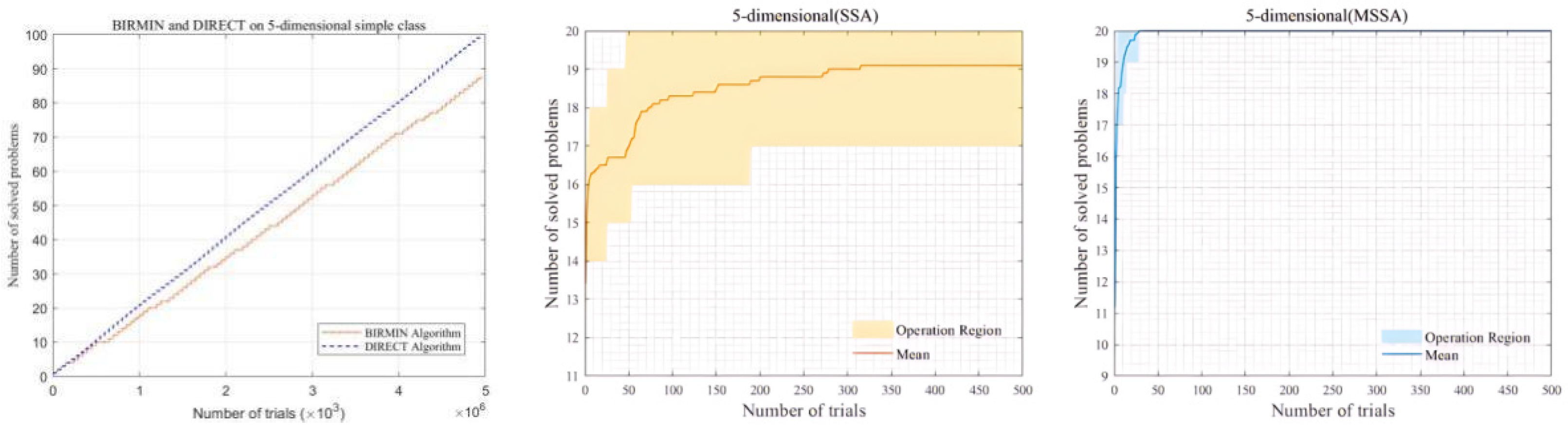
- Based on the tests conducted on 23 benchmark functions, CEC2019 test functions, and three engineering optimization problems, the MSSA was also compared with the deterministic algorithms DIRECT and BRIMIN on 100 five-dimensional GKLS test functions to verify its global optimization ability.
- (3)
- The algorithm’s effectiveness is verified through statistical analysis of mean and standard deviation. The Wilcoxon’s rank-sum test at a 0.05 significance level shows a significant difference.
- (4)
- The modified MSSA is applied to a 20 × 20 robot path planning problem, validating its performance in dynamic obstacle avoidance and path optimization, providing strong algorithmic support for practical applications.
2. Sparrow Search Algorithm (SSA)
2.1. Producer Position Updates Phase
2.2. Scrounger Position Updates Phase
2.3. Scouter Position Updates Phase
3. A Modified Sparrow Search Algorithm
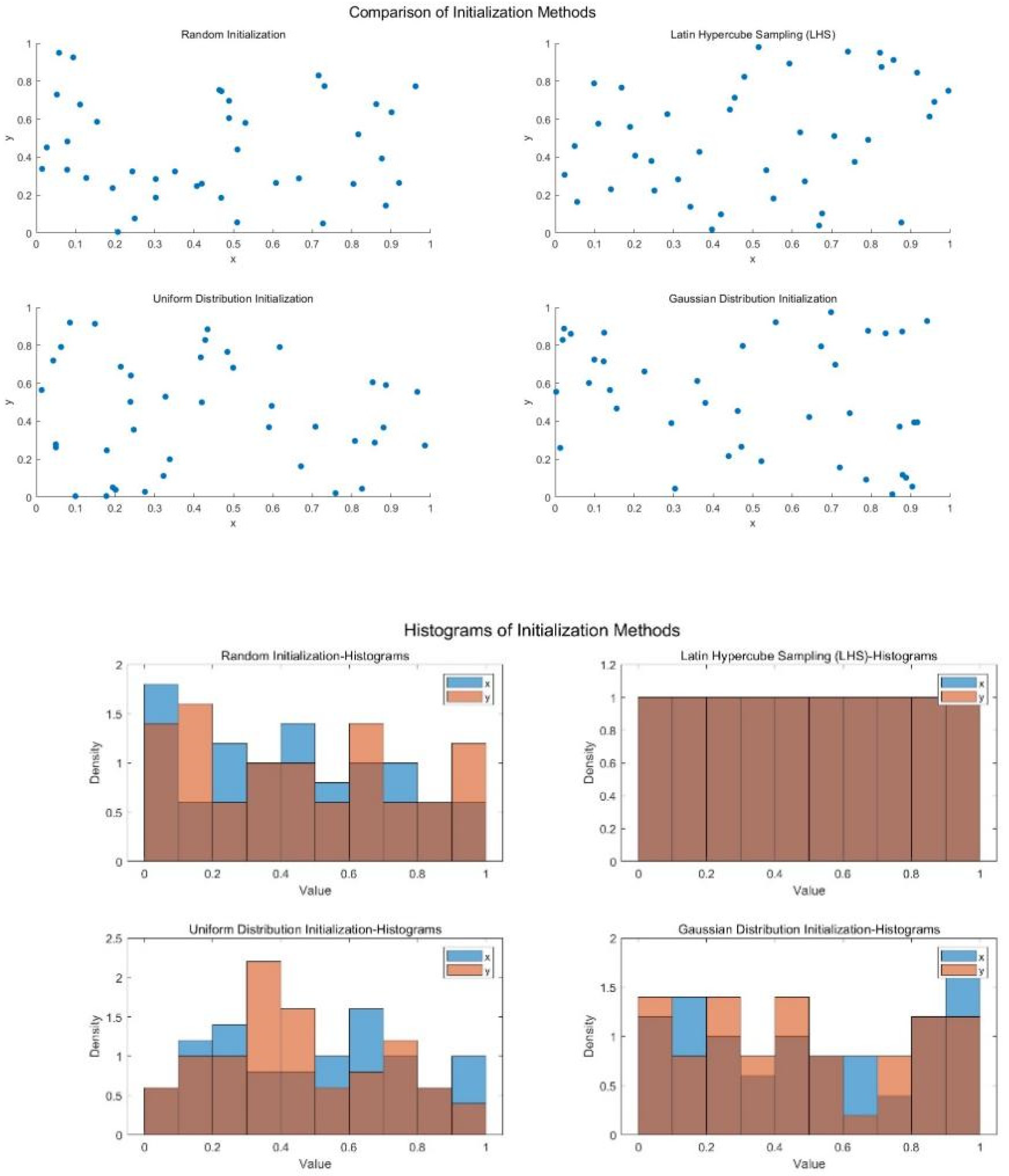
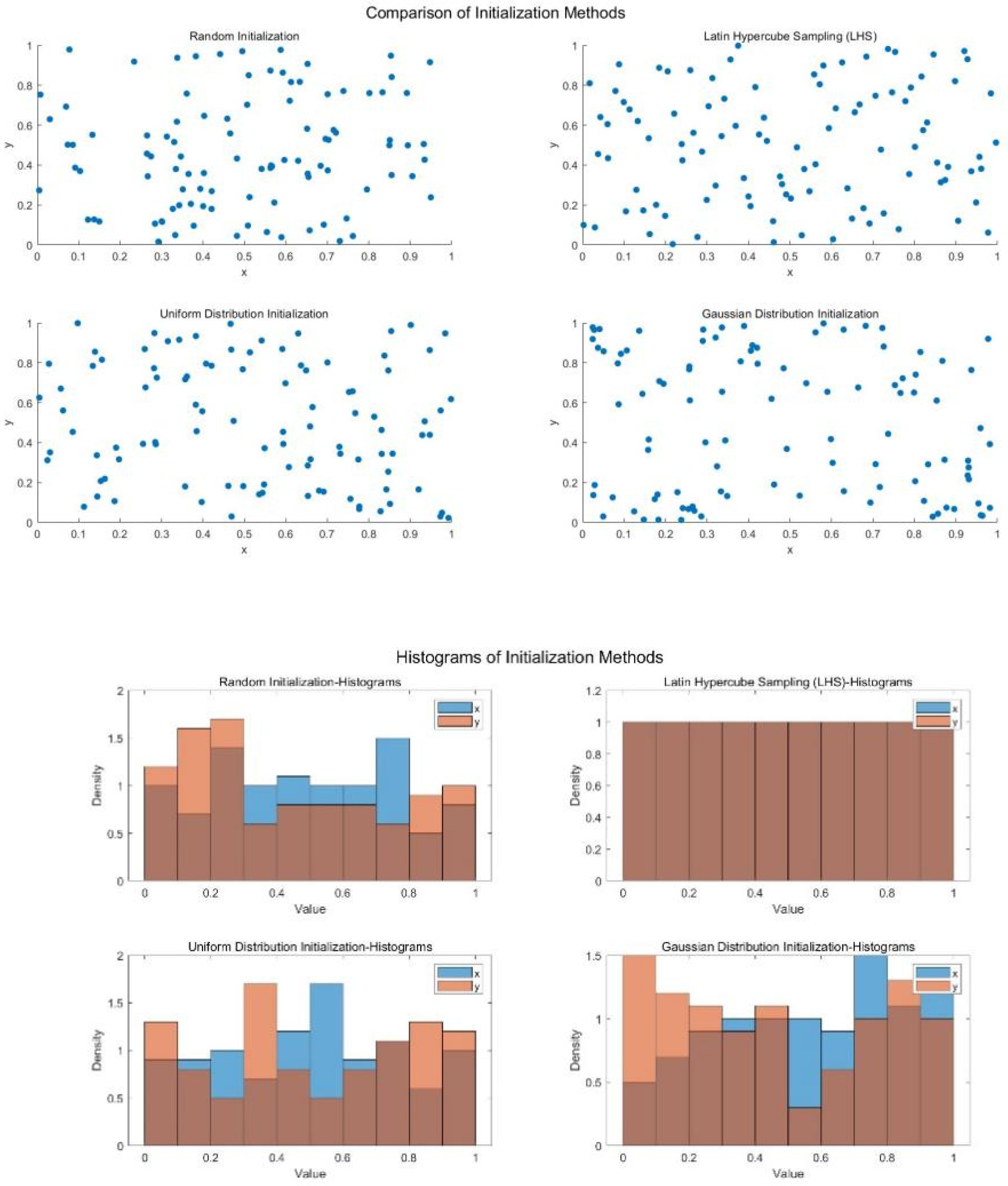
3.1. Latin Hypercube Sampling
- (1)
- First, determine the population size and the dimensionality of the population.
- (2)
- Define the range of variables as , where and are the upper and lower bounds, respectively.
- (3)
- Divide the range of each variable into equal intervals. The width of each sub-interval is .
- (4)
- Randomly select a point from each interval in every dimension. A random number generator within the range of [0, 1] can be used in each sub-interval.
- (5)
- Combine the points selected in all dimensions to form the initial population. After sampling one point in each sub-interval of all dimensions, an individual in the population is formed. Repeat this process times to obtain the initial population of the MSSA algorithm.
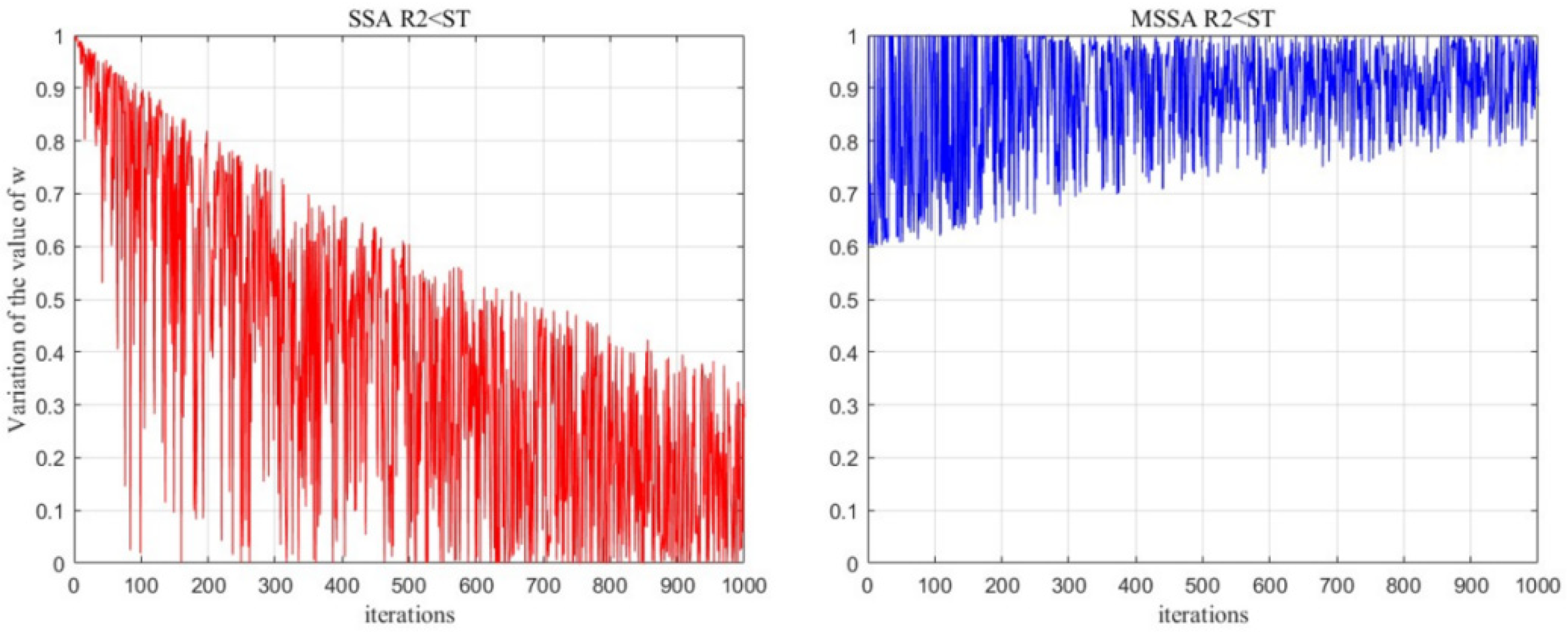
3.2. Adaptive Weighting Mechanism
3.3. Cauchy Mutation and Cat Disturbance Strategy
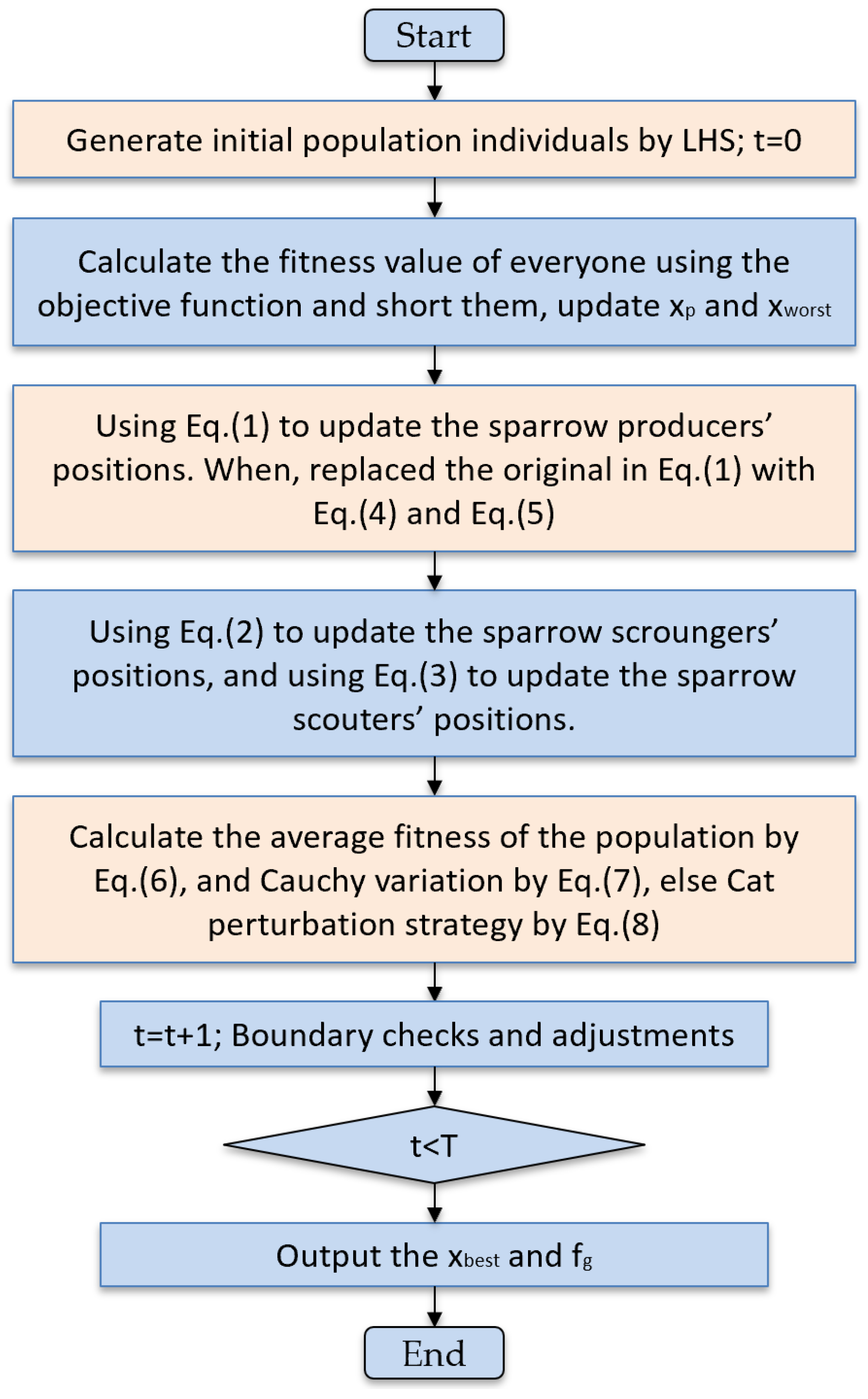
| Algorithm 1: Pseudo-code of MSSA |
| Input: , , , , , , Initialized population individuals generated Latin hypercube sampling (LHS) within the dimensional problem space. |
| Output: , 1: While do 2: Rank the fitness values, identify the current best individual and worst individuals , 3: for 4: Using Equation (1) to update the sparrow producers’ positions. When , replaced the original in Equation (1) with Equation (4) and Equation (5). 5: end for 6: for 7: Using Equation (2) to update the sparrow scroungers’ positions. 8: for 9: Using Equation (3) to update the sparrow producers’ positions. 10: end for 11: Calculating the average fitness of the population by Equation (6). 12: if 13: Cauchy variation by Equation (7) was employed to perturb sparrow populations in instances where the fitness of individual sparrows fell below the average fitness. 14: else 15: Sparrow populations were perturbed utilizing the Cat perturbation strategy by Equation (8). 16: Boundary checks and adjustments 17: Obtain the current new location; 18: If the current new location is superior to the previous one, update it; 19: 20: end while 21: return , . |
3.4. Complexity Analysis
4. Performance Testing of Functions
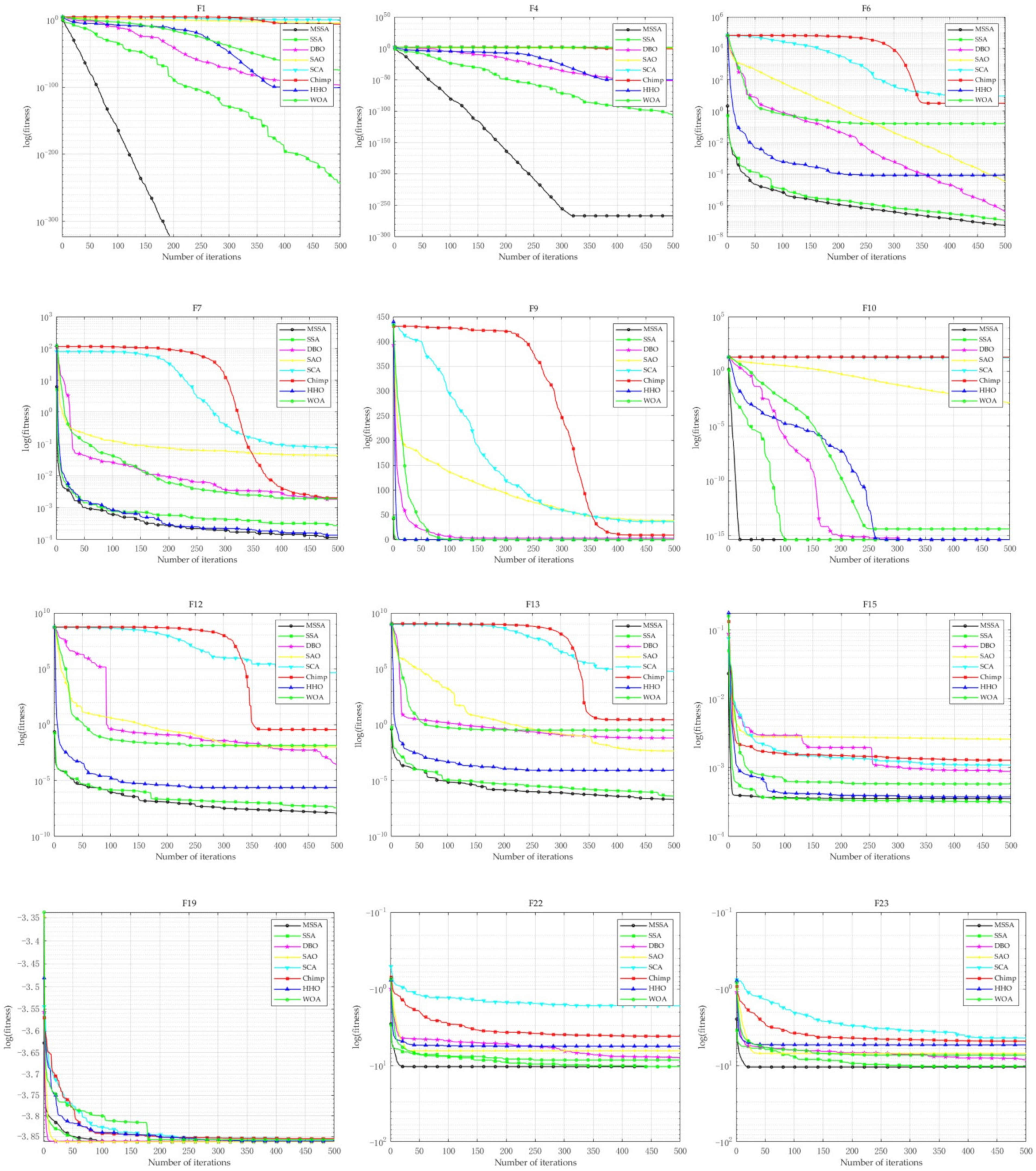
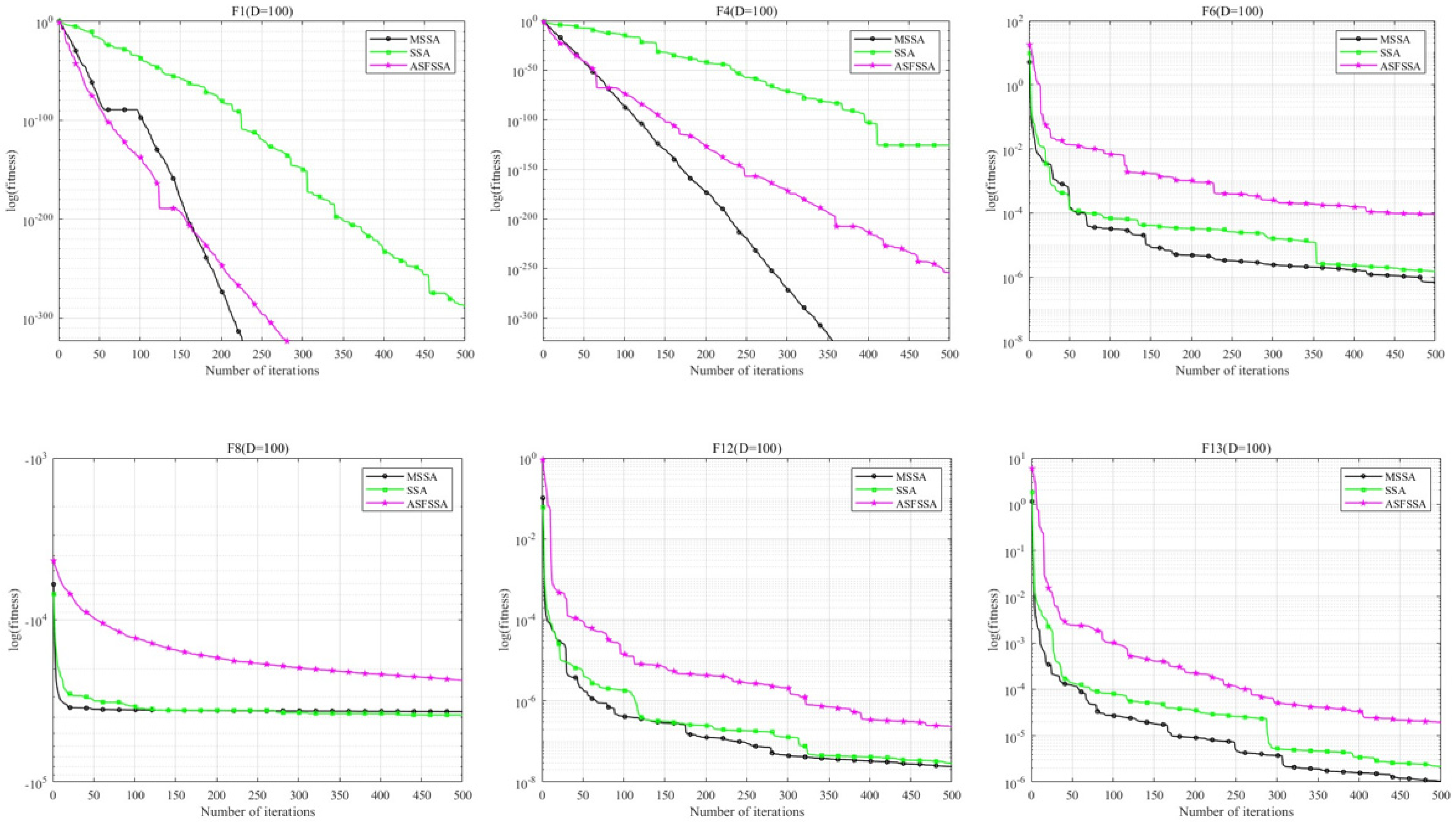
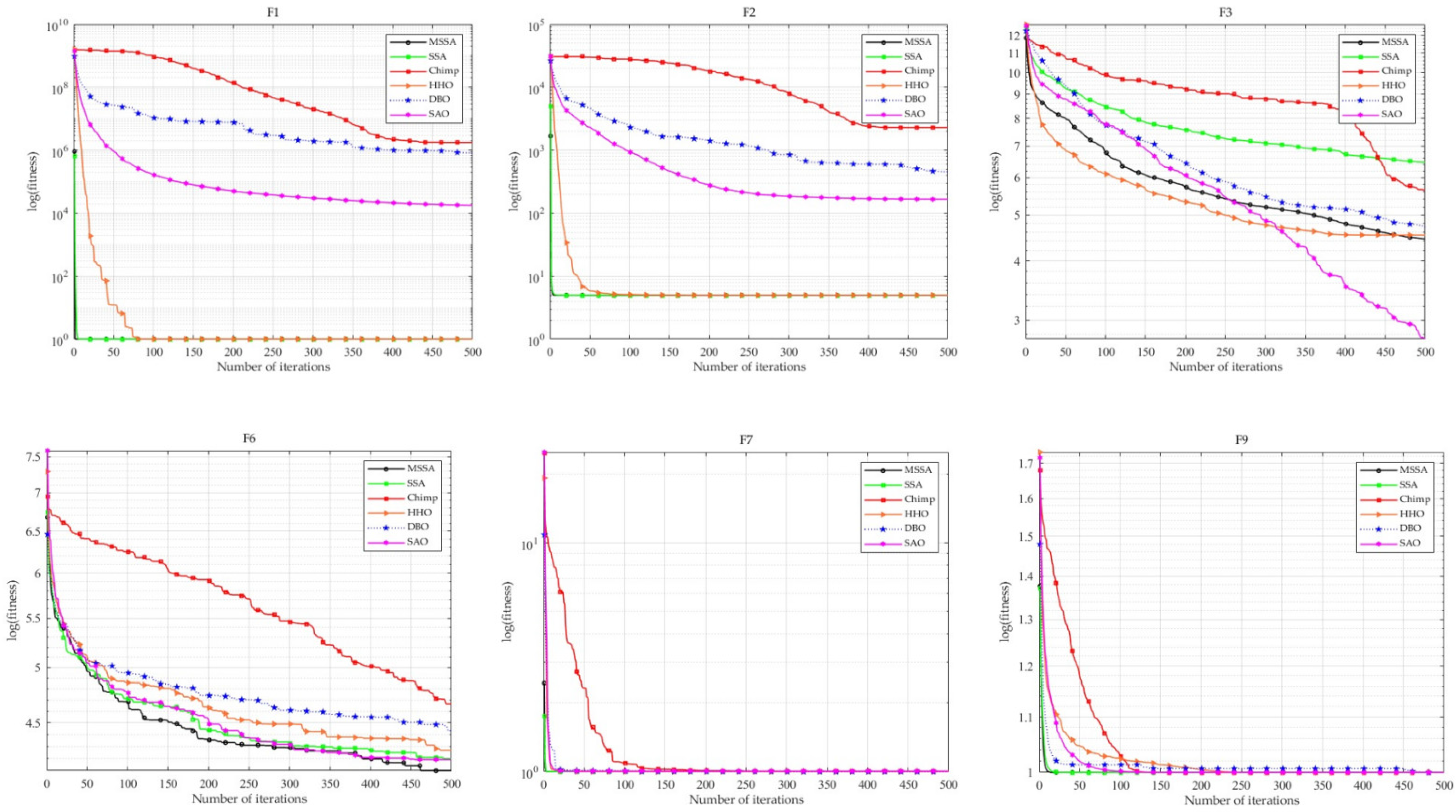
4.1. Performance Testing on 23 Benchmark Functions
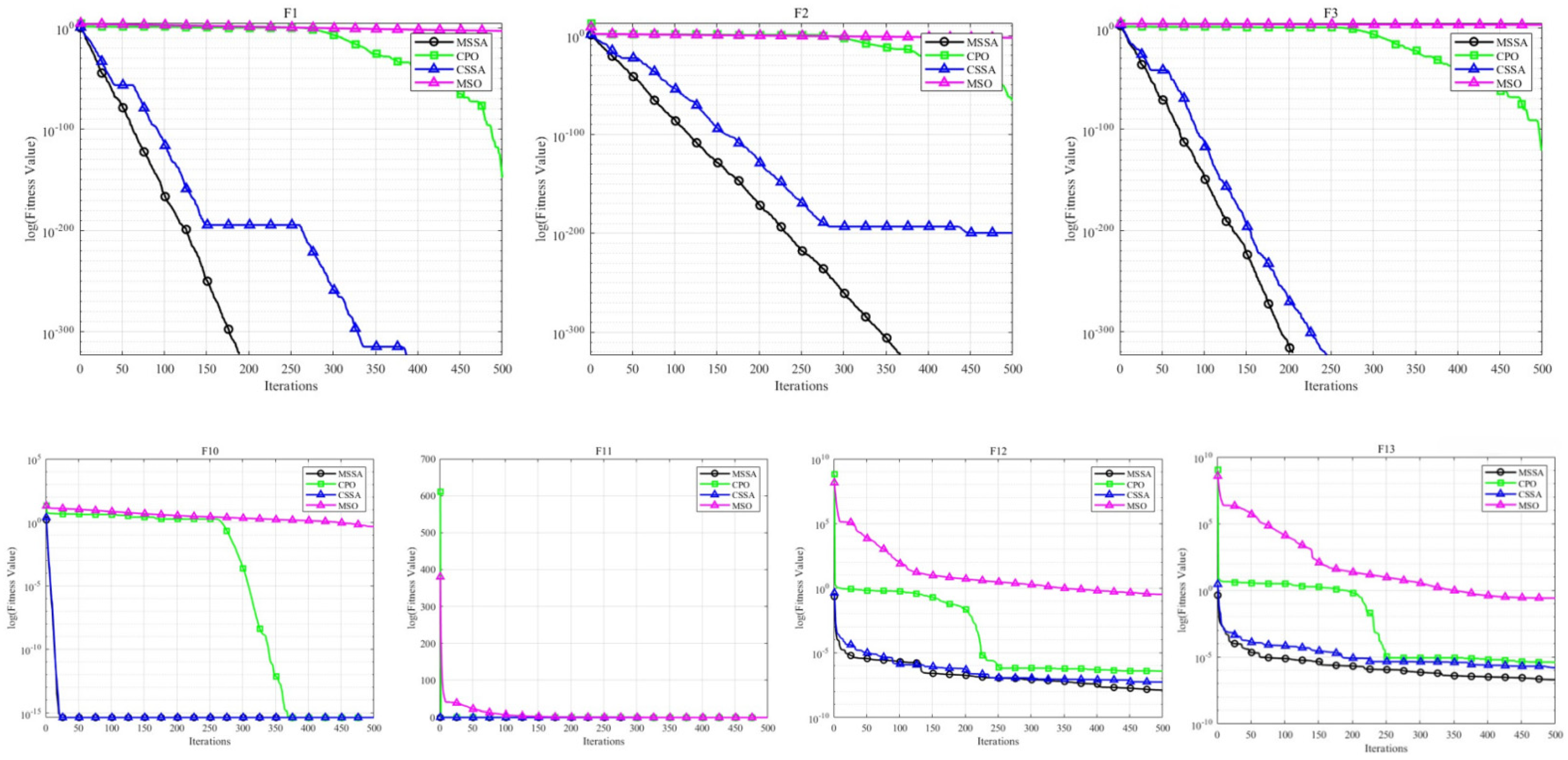
4.2. Performance Testing on CEC2019
4.3. Performance Testing on GKLS Functions
5. Performance on Engineering Optimization Problems
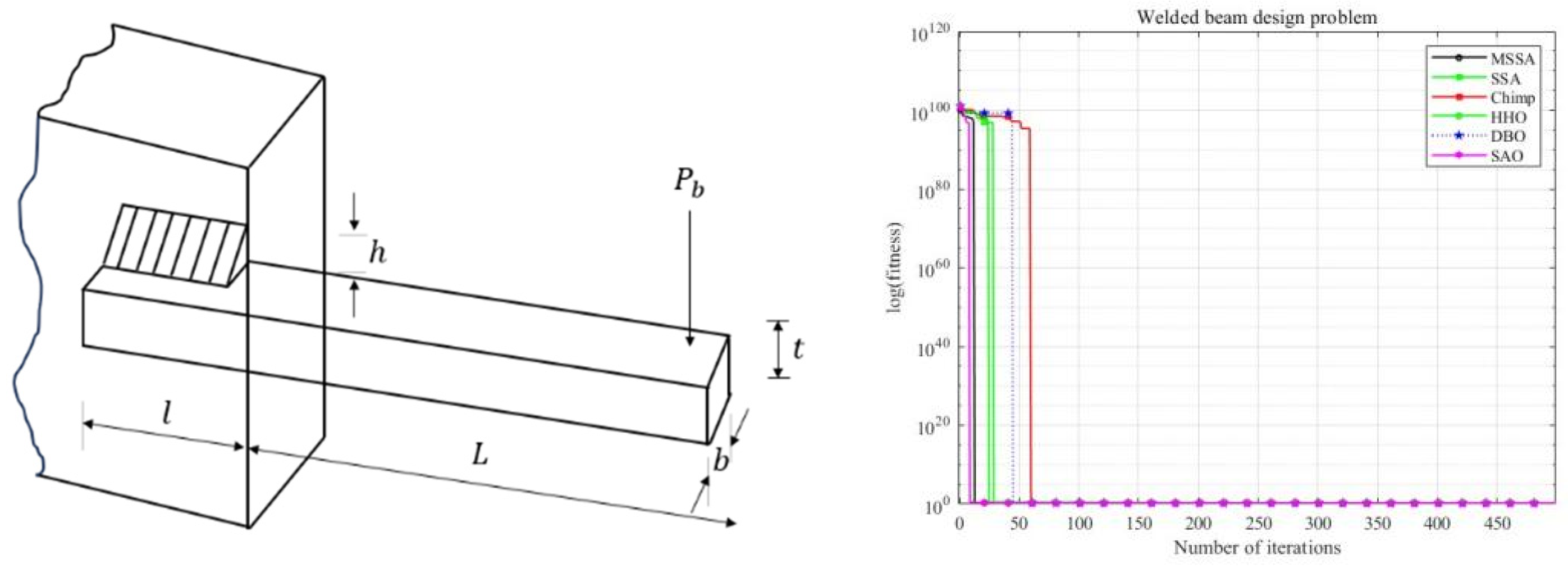
5.1. Welded Beam Design Problem
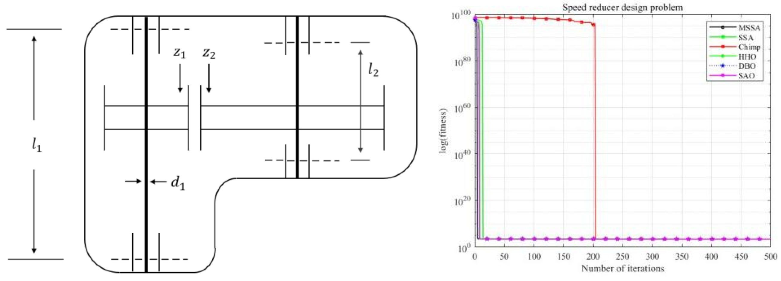
5.2. Speed Reducer Design Problem
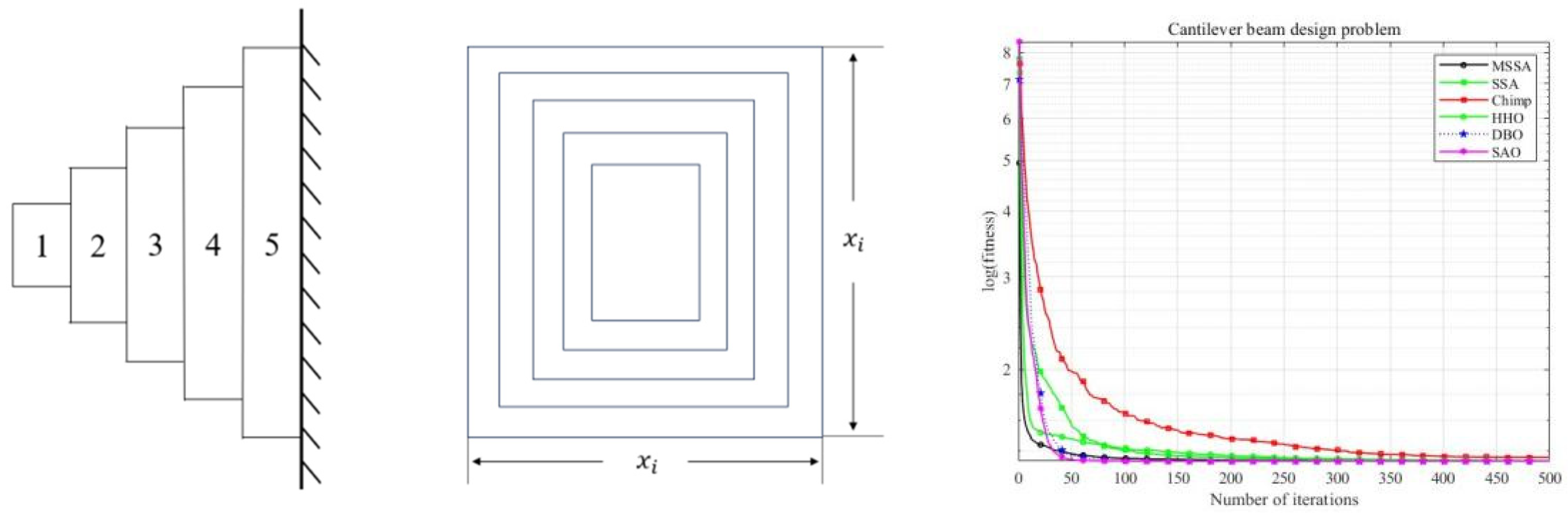
5.3. Cantilever Beam Design Problem
6. Robot Path Planning Based on MSSA
6.1. Experimental Environment Settings
6.2. Simulation Results and Analysis
7. Conclusions
Author Contributions
Funding
Institutional Review Board Statement
Informed Consent Statement
Data Availability Statement
Conflicts of Interest
References
- Yun, L. MATLAB implementation of Newton’s iteration method. Inf. Commun. 2011, 24, 20–22. [Google Scholar]
- Ruder, S. An overview of gradient descent optimization algorithms. arXiv 2016, arXiv:1609.04747. [Google Scholar]
- Cao, L.; Cai, Y.; Yue, Y. Swarm Intelligence-Based Performance Optimization for Mobile Wireless Sensor Networks: Survey, Challenges, and Future Directions. IEEE Access 2019, 7, 161524–161553. [Google Scholar] [CrossRef]
- Zhang, J.J.; Li, J.D.; Xu, X.M. A Passive Positioning Algorithm Using Time-Frequency Differences Based on the Cuckoo Search Algorithm and the Newton Method. Electron. Des. Eng. 2023, 31, 78–82. [Google Scholar]
- Izuchukwu, C.; Shehu, Y. A new inertial projected reflected gradient method with application to optimal control problems. Optim. Methods Softw. 2023, 39, 197–226. [Google Scholar] [CrossRef]
- Sakovich, N.; Aksenov, D.; Pleshakova, E.; Gataullin, S. MAMGD: Gradient-Based Optimization Method Using Exponential Decay. Technologies 2024, 12, 154. [Google Scholar] [CrossRef]
- Yan, F.; Xu, Y. An Optimized MTD Moving Target Detection Algorithm Based on Gradient Descent with Sampling Point Weights. In Proceedings of the 22nd Academic Annual Conference on Vacuum Electronics, Online, 27–30 April 2021; pp. 509–513. [Google Scholar]
- Ye, R.Z.; Du, F.Z. A Multi-Objective Fuzzy Optimization Scheduling Method for Regional Power Grids Based on the Distributed Newton Method. Electr. Technol. Econ. 2024, 299–302. [Google Scholar]
- Kennedy, J. Particle Swarm Optimization. In Proceedings of the 1995 IEEE International Conference on Neural Networks, Perth, WA, Australia, 27 November–1 December 2011; Volume 4, pp. 1942–1948. [Google Scholar]
- Han, Y.; Cai, J.; Zhou, G.; Li, Y.; Lin, H.; Tang, J. Research Progress of Random Frog Leaping Algorithm. Comput. Sci. 2010. [Google Scholar]
- Qin, Q.; Cheng, S.; Li, L.; Shi, Y. Artificial Bee Colony Algorithm: A Survey. Appl. Math. Comput. 2014, 249, 126–141. [Google Scholar]
- Mirjalili, S.; Mirjalili, S.M.; Lewis, A. Grey Wolf Optimizer. Adv. Eng. Softw. 2014, 69, 46–61. [Google Scholar] [CrossRef]
- Mirjalili, S. SCA: A Sine Cosine Algorithm for Solving Optimization Problems. Knowl.-Based Syst. 2016, 96, 120–133. [Google Scholar] [CrossRef]
- Mirjalili, S.; Lewis, A. The Whale Optimization Algorithm. Adv. Eng. Softw. 2016, 95, 51–67. [Google Scholar] [CrossRef]
- Heidari, A.A.; Mirjalili, S.; Faris, H.; Aljarah, I.; Mafarja, M.; Chen, H. Harrishawks Optimization: Algorithm and Applications. Fut. Gener. Comput. Syst. 2019, 97, 849–872. [Google Scholar] [CrossRef]
- Khishe, M.; Mosavi, M.R. Chimp Optimization Algorithm. Expert Syst. Appl. 2020, 149, 113338. [Google Scholar] [CrossRef]
- Xue, J.; Shen, B. A novel swarm intelligence optimization approach: Sparrow search algorithm. Syst. Sci. Control. Eng. 2020, 8, 22–34. [Google Scholar] [CrossRef]
- Xue, J.; Shen, B. Dung beetle optimizer: A new meta-heuristic algorithm for global optimization. J. Supercomput. 2022, 79, 1–32. [Google Scholar] [CrossRef]
- Deng, L.; Liu, S. Snow Ablation Optimizer: A Novel Metaheuristic Technique for Numerical Optimization and Engineering Design. Expert. Syst. Appl. 2023, 225, 120069. [Google Scholar] [CrossRef]
- Guo, Z.; Liu, G.; Jiang, F. Chinese Pangolin Optimizer: A novel bio-inspired metaheuristic for solving optimization problems. J. Supercomput. 2025, 81, 517. [Google Scholar] [CrossRef]
- He, J.; Zhao, S.; Ding, J.; Wang, Y. Mirage search optimization: Application to path planning and engineering design problems. Adv. Eng. Softw. 2025, 203, 103883. [Google Scholar] [CrossRef]
- Elsisi, M. Optimal Design of Adaptive Model Predictive Control Based on Improved GWO for Autonomous Vehicle Considering System Vision Uncertainty. Appl. Soft Comput. 2024, 158, 111581. [Google Scholar] [CrossRef]
- Chen, M.; Cheng, Q.; Feng, X.; Zhao, K.; Zhou, Y.; Xing, B.; Tang, S.; Wang, R.; Duan, J.; Wang, J.; et al. Optimized variational mode decomposition algorithm based on adaptive thresholding method and improved whale optimization algorithm for denoising magnetocardiography signal. Biomed. Signal Process. Control. 2024, 88, 105681. [Google Scholar] [CrossRef]
- Liu, H.; Fan, J.; Guo, P. Improved gorilla optimization algorithm for kernel fuzzy clustering segmentation of RGB-D images. Microelectron. Comput. 2024, 1, 1–12. [Google Scholar]
- Javaheri, D.; Gorgin, S.; Lee, J.A.; Masdari, M. An improved discrete Harris hawk optimization algorithm for efficient workflow scheduling in multi-fog computing. Expert. Syst. Appl. 2021, 166, 113917. [Google Scholar] [CrossRef]
- Zhang, C.; Ma, H.; Hua, L.; Sun, W.; Nazir, M.S.; Peng, T. An evolutionary deep learning model based on TVFEMD, improved sine cosine algorithm, CNN and BiLSTM for wind speed prediction. Renew. Energy 2022, 187, 1107–1118. [Google Scholar] [CrossRef]
- Wu, D.; Yuan, C. Correction to: Threshold image segmentation based on improved sparrow search algorithm. Multimed. Tools Appl. 2022, 81, 33513–33546. [Google Scholar] [CrossRef] [PubMed]
- Panimalar, K.; Kanmani, S. Energy Efficient Cluster Head Selection Using Improved Sparrow Search Algorithm in Wireless Sensor Networks. J. King Saud Univ. Comput. Inf. Sci. 2022, 34, 8564–8575. [Google Scholar]
- Fei, L.; Li, R.; Liu, S.Q.; Tang, B.; Li, S.; Masoud, M. An Improved Sparrow Search Algorithm for Solving the Energy-Saving Flexible Job Shop Scheduling Problem. Machines 2022, 10, 847. [Google Scholar] [CrossRef]
- Zhou, N.; Zhang, S.; Zhang, C. Multi Strategy Improved Sparrow Search Algorithm Based on Rough Data Reasoning. J. Univ. Electron. Sci. Technol. China 2022, 51, 743–753. [Google Scholar]
- Zhang, W.; Liu, S. Adaptive t-Distribution and Improved Golden Sine Sparrow Search Algorithm and Its Applications. Microelectron. Comput. 2022, 39, 17–24. [Google Scholar]
- Ouyang, C.; Qiu, Y.; Zhu, D. Adaptive Spiral Flying Sparrow Search Algorithm. Sci. Prog. 2021, 2021, 1–16. [Google Scholar] [CrossRef]
- Duan, Y.; Liu, C. Sparrow Search Algorithm Based on Sobol Sequence and Crisscross Strategy. J. Comput. Appl. 2022, 42, 36–43. [Google Scholar]
- Zhang, C.; Ding, S. A Stochastic Configuration Network Based on Chaotic Sparrow Search Algorithm. Knowl. Based Syst. 2021, 220, 106924. [Google Scholar] [CrossRef]
- Zhu, Y.; Yousefi, N. Optimal Parameter Identification of PEMFC Stacks Using Adaptive Sparrow Search Algorithm. Microelectron. Comput. 2021, 39, 17–24. [Google Scholar] [CrossRef]
- Liu, G.; Shu, C.; Liang, Z.; Peng, B.; Cheng, L. A Modified Sparrow Search Algorithm with Application in 3D Route Planning for UAV. Sensors 2021, 21, 1224. [Google Scholar] [CrossRef] [PubMed]
- Song, X.; Wu, Q.; Cai, Y. Short-Term Power Load Forecasting Based on GRU Neural Network Optimized by an Improved Sparrow Search Algorithm. In Proceedings of the Eighth International Symposium on Advances in Electrical, Electronics, and Computer Engineering (ISAEECE 2023), Hangzhou, China, 17–19 February 2023; p. 1270431. [Google Scholar]
- Wolpert, D.H.; Macready, W.G. No Free Lunch Theorems for Optimization. IEEE Trans. Evol. Comput. 1997, 1, 67–82. [Google Scholar] [CrossRef]
- Stein, M. Large Sample Properties of Simulations Using Latin Hypercube Sampling. Technometrics 1987, 29, 143–151. [Google Scholar] [CrossRef]
- Lü, L.; Ji, W. A Particle Swarm Optimization Algorithm Combining Centroid Concept and Cauchy Mutation Strategy. Comput. Appl. 2017, 37, 1369–1375. [Google Scholar]
- Han, R.; Zhang, X.F. Pseudo-random sequence generation method based on high-dimensional cat mapping. Comput. Eng. Appl. 2016, 52, 91–99. [Google Scholar]
- Suganthan, P.N.; Hansen, N.; Liang, J.J.; Deb, K.; Chen, Y.-P.; Auger, A.; Tiwari, S. Problem Definitions and Evaluation Criteria for the CEC 2005 Special Session on Real-Parameter Optimization. Nat. Comput. 2005, 341–357. [Google Scholar]
- Price, K.V.; Awad, N.H.; Ali, M.Z.; Suganthan, P.N. Problem Definitions and Evaluation Criteria for the 100-Digit Challenge Special Session and Competition on Single Objective Numerical Optimization; Technical Report; Nanyang Technological University: Singapore, 2018. [Google Scholar]
- Gaviano, M.; Kvasov, D.E.; Lera, D.; Sergeyev, Y.D. Algorithm 829: Software for generation of classes of test functions with known local and global minima for global optimization. ACM Trans. Math. Softw. 2003, 29, 469–480. [Google Scholar] [CrossRef]
- Sergeyev, Y.D.; Kvasov, D.E.; Mukhametzhanov, M.S. On the efficiency of nature-inspired metaheuristics in expensive global optimization with limited budget. Sci. Rep. 2018, 8, 453. [Google Scholar] [CrossRef] [PubMed]
- Rather, S.A.; Bala, P.S. Swarm-Based Chaotic Gravitational Search Algorithm for Solving Mechanical Engineering Design Problems. World J. Eng. 2020, 17, 97–114. [Google Scholar] [CrossRef]
- Chen, P.; Zhou, S.; Zhang, Q.; Kasabov, N. A Meta-Inspired Termite Queen Algorithm for Global Optimization and Engineering Design Problems. Eng. Appl. Artif. Intell. 2022, 111, 104805. [Google Scholar] [CrossRef]
- Zhao, Z.H.; Ma, J.D.; Zhang, Y.R. Research on Robot Path Planning Based on an Improved Particle Swarm Dung Beetle Algorithm. China New Technol. Prod. 2024, 46. [Google Scholar]


| Sampling Methods | Characteristics | Advantages | Disadvantages |
|---|---|---|---|
| Random Sampling | Samples are randomly distributed within the interval. | Easy to implement, suitable for large-scale sampling. | Samples may cluster in some areas, leading to uneven coverage. |
| Latin Hypercube Sampling (LHS) | Multidimensional stratified | Can effectively cover the entire range even with few samples. | More complex to compute compared to the tails. |
| Uniform Distribution Sampling | Each point in the interval has the same probability of being selected. | Simple and easy to implement. | Samples may cluster in certain areas, resulting in uneven coverage. |
| Gaussian Distribution Sampling | Samples are distributed around the mean, with fewer samples far from the mean. | Suitable for normally distributed data, easy to generate. | Samples are concentrated near the mean, with sparse coverage in the tails. |
| Algorithm | Parameters | Population |
|---|---|---|
| SCA | Population = 40 | |
| WOA | , , linearly decrease | |
| HHO | ||
| Chimp | ||
| SSA | , , | |
| ASFSSA | , , | |
| DBO | , , , , | |
| SAO | ||
| GA | ||
| CPO | ||
| MSO |
| Function | Parameters | SSA | DBO | SAO | SCA | Chimp | HHO | WOA | MSSA | |
|---|---|---|---|---|---|---|---|---|---|---|
| Uni-modal functions | F1 | Mean | 4.8403 × 10−244 | 1.6633 × 10−97 | 3.9791 × 10⁻⁵ | 3.026 | 8.0807 × 10⁻⁷ | 1.2148 × 10−101 | 4.5632 × 10−75 | 0 |
| SD | 0 | 7.4385 × 10−97 | 6.0809 × 10⁻⁵ | 5.2634 | 2.0318 × 10⁻⁶ | 4.7343 × 10−101 | 2.0406 × 10−74 | 0 | ||
| p-values | 0.125 | 8.8575 × 10⁻⁵ | 8.8575 × 10⁻⁵ | 8.8575 × 10⁻⁵ | 8.8575 × 10⁻⁵ | 8.8575 × 10⁻⁵ | 8.8575 × 10⁻⁵ | NA | ||
| F2 | Mean | 1.1962 × 10⁻⁷ | 2.8036 × 10−65 | 8.8091 × 10⁻⁴ | 1.5654 × 10⁻² | 7.0217 × 10⁻⁶ | 5.5887 × 10−52 | 1.9709 × 10−53 | 1.2942 × 10−273 | |
| SD | 2.6373 × 10⁻⁷ | 1.2459 × 10−64 | 1.3044 × 10⁻³ | 3.2183 × 10⁻² | 8.563 × 10⁻⁶ | 2.2355 × 10−51 | 5.9608 × 10−53 | 0 | ||
| p-values | 3.5153 × 10⁻⁴ | 8.8575 × 10⁻⁵ | 8.8575 × 10⁻⁵ | 8.8575 × 10⁻⁵ | 8.8575 × 10⁻⁵ | 8.8575 × 10⁻⁵ | 8.8575 × 10⁻⁵ | NA | ||
| F3 | Mean | 9.0416 × 10−268 | 2.3775 × 10-83 | 1066.3701 | 5856.0238 | 154.2924 | 1.917 × 10−83 | 33,479.2865 | 0 | |
| SD | 0 | 1.0602 × 10−82 | 1446.7758 | 3755.2895 | 435.3517 | 8.1173 × 10−83 | 13,578.1384 | 0 | ||
| p-values | 3.125 × 10⁻² | 8.8575 × 10⁻⁵ | 8.8575 × 10⁻⁵ | 8.8575 × 10⁻⁵ | 8.8575 × 10⁻⁵ | 8.8575 × 10⁻⁵ | 8.8575 × 10⁻⁵ | NA | ||
| F4 | Mean | 3.3225 × 10−107 | 4.4094 × 10−52 | 1.423 | 30.1469 | 0.11623 | 1.0448 × 10−50 | 47.6442 | 3.2137 × 10−267 | |
| SD | 1.4859 × 10−106 | 1.8761 × 10−51 | 0.57081 | 10.4015 | 8.5933 × 10⁻² | 2.8154 × 10−50 | 31.7755 | 0 | ||
| p-values | 4.3778 × 10⁻⁴ | 8.8575 × 10⁻⁵ | 8.8575 × 10⁻⁵ | 8.8575 × 10⁻⁵ | 8.8575 × 10⁻⁵ | 8.8575 × 10⁻⁵ | 8.8575 × 10⁻⁵ | NA | ||
| F5 | Mean | 2.0593 × 10⁻⁵ | 25.4035 | 40.4379 | 43,449.6197 | 28.8927 | 4.184 × 10⁻³ | 27.8302 | 7.7089 × 10⁻⁶ | |
| SD | 5.3199 × 10⁻⁵ | 0.22367 | 27.6976 | 120,561.791 | 9.5663 × 10⁻² | 6.0131 × 10⁻³ | 0.47304 | 1.8361 × 10⁻⁵ | ||
| p-values | 0.16718 | 8.8575 × 10⁻⁵ | 8.8575 × 10⁻⁵ | 8.8575 × 10⁻⁵ | 8.8575 × 10⁻⁵ | 1.0335 × 10⁻⁴ | 8.8575 × 10⁻⁵ | NA | ||
| F6 | Mean | 1.1962 × 10⁻⁷ | 4.0449 × 10⁻⁷ | 3.3332 × 10⁻⁵ | 9.1999 | 3.1781 | 8.4771 × 10⁻⁵ | 0.16175 | 5.3953 × 10⁻⁸ | |
| SD | 2.6373 × 10⁻⁷ | 5.2474 × 10⁻⁷ | 3.0624 × 10⁻⁵ | 7.6902 | 0.44439 | 1.6742 × 10⁻⁴ | 0.1323 | 1.1408 × 10⁻⁷ | ||
| p-values | 0.64416 | 6.8061 × 10⁻⁴ | 8.8575 × 10⁻⁵ | 8.8575 × 10⁻⁵ | 8.8575 × 10⁻⁵ | 8.8575 × 10⁻⁵ | 8.8575 × 10⁻⁵ | NA | ||
| F7 | Mean | 2.741 × 10⁻⁴ | 1.8578 × 10⁻³ | 0.4284 | 7.5726 × 10⁻² | 2.0733 × 10⁻³ | 1.3783 × 10⁻⁴ | 1.9485 × 10⁻³ | 1.1603 × 10⁻⁴ | |
| SD | 2.493 × 10⁻⁴ | 1.2634 × 10⁻³ | 1.7508 × 10⁻² | 7.8847 × 10⁻² | 1.8934 × 10⁻³ | 1.6957 × 10⁻⁴ | 1.6768 × 10⁻³ | 8.5419 × 10⁻⁵ | ||
| p-values | 4.7858 × 10⁻² | 8.8575 × 10⁻⁵ | 8.8575 × 10⁻⁵ | 8.8575 × 10⁻⁵ | 8.8575 × 10⁻⁵ | 0.88129 | 1.6286 × 10⁻⁴ | NA | ||
| Multi-modal functions | F8 | Mean | −9502.1132 | −8870.9105 | −9120.8181 | −3768.5139 | −5730.4026 | −12,569.1605 | −10,973.321 | −10,879.7721 |
| SD | 2738.0434 | 1446.006 | 772.1644 | 243.0804 | 62.194 | 0.54721 | 2094.2708 | 1794.4138 | ||
| p-values | 0.21796 | 5.734 × 10⁻³ | 2.495 × 10⁻³ | 8.8575 × 10⁻⁵ | 1.0335 × 10⁻⁴ | 8.8575 × 10⁻⁵ | 0.68132 | NA | ||
| F9 | Mean | 0 | 2.4898 | 38.1862 | 36.0641 | 9.075 | 0 | 0 | 0 | |
| SD | 0 | 6.8064 | 15.5384 | 38.0386 | 7.8769 | 0 | 0 | 0 | ||
| p-values | 1 | 0.125 | 8.8575 × 10⁻⁵ | 8.8575 × 10⁻⁵ | 8.8575 × 10⁻⁵ | 1 | 1 | NA | ||
| F10 | Mean | 4.4409 × 10⁻¹⁶ | 4.4409 × 10⁻¹⁶ | 1.4674 × 10⁻³ | 16.5063 | 19.9622 | 4.4409 × 10⁻¹⁶ | 2.7534 × 10⁻¹⁵ | 4.4409 × 10⁻¹⁶ | |
| SD | 0 | 0 | 1.459 × 10⁻³ | 7.6507 | 1.3489 × 10⁻³ | 0 | 1.7386 × 10⁻¹⁵ | 4.4409 × 10⁻¹⁶ | ||
| p-values | 1 | 1 | 8.8575 × 10⁻⁵ | 8.8575 × 10⁻⁵ | 8.8575 × 10⁻⁵ | 1 | 2.4414 × 10⁻⁴ | NA | ||
| F11 | Mean | 0 | 0 | 5.2997 × 10⁻² | 0.7005 | 2.5468 × 10⁻² | 0 | 4.2266 × 10⁻³ | 0 | |
| SD | 0 | 0 | 2.0365 × 10⁻¹ | 0.31924 | 4.3681 × 10⁻² | 0 | 1.8902 × | 0 | ||
| p-values | 1 | 1 | 8.8575 × 10⁻⁵ | 8.8575 × 10⁻⁵ | 8.8575 × 10⁻⁵ | 1 | 1 | NA | ||
| F12 | Mean | 3.6802 × 10⁻⁸ | 2.6807 × 10⁻⁴ | 1.0371 × 10⁻² | 45,201.469 | 0.3697 | 2.4008 × 10⁻⁶ | 1.3899 × 10⁻² | 1.2762 × 10⁻⁸ | |
| SD | 6.6565 × 10⁻⁸ | 1.1283 × 10⁻³ | 3.1908 × 10⁻² | 202,001.79 | 0.14812 | 2.5829 × 10⁻⁶ | 1.0749 × 10⁻² | 1.5159 × 10⁻⁸ | ||
| p-values | 0.29588 | 5.6915 × 10⁻² | 8.8575 × 10⁻⁵ | 8.8575 × 10⁻⁵ | 8.857 × 10⁻⁵ | 8.8575 × 10⁻⁵ | 8.8575 × 10⁻⁵ | NA | ||
| F13 | Mean | 4.1787 × 10⁻⁷ | 6.527 × 10⁻² | 4.4476 × 10⁻³ | 60,807.8872 | 2.7933 | 8.5529 × 10⁻⁵ | 0.32628 | 2.1011 × 10⁻⁷ | |
| SD | 6.2505 × 10⁻⁷ | 0.11389 | 0.10309 | 164,292.136 | 0.12083 | 6.9127 × 10⁻⁵ | 0.1877 | 4.1398 × 10⁻⁷ | ||
| p-values | 3.6561 × 10⁻² | 8.8575 × 10⁻⁵ | 1.4013 × 10⁻⁴ | 8.8575 × 10⁻⁵ | 8.8575 × 10⁻⁵ | 1.0335 × 10⁻⁴ | 8.8575 × 10⁻⁵ | NA | ||
| Fixed-dimensional multi-modal functions | F14 | Mean | 7.1949 | 1.1964 | 3.0155 | 1.891 | 0.99812 | 1.4931 | 2.6614 | 0.998 |
| SD | 5.0208 | 0.61069 | 3.0155 | 1.0126 | 4.3042 × 10⁻⁴ | 1.1321 | 3.5292 | 2.3447 × 10⁻⁹ | ||
| p-values | 1.1529 × 10⁻⁴ | 0.72656 | 4.8828 × 10⁻⁴ | 8.8575 × 10⁻⁵ | 8.8575 × 10⁻⁵ | 6.8061 × 10⁻⁴ | 5.9342 × 10⁻⁴ | NA | ||
| F15 | Mean | 3.1787 × 10⁻⁴ | 8.648 × 10⁻⁴ | 2.5917 × 10⁻³ | 1.0903 × 10⁻³ | 1.2823 × 10⁻³ | 3.762 × 10⁻⁴ | 5.7833 × 10⁻⁴ | 3.5493 × 10⁻⁴ | |
| SD | 2.0142 × 10⁻⁵ | 3.2621 × 10⁻⁴ | 6.0923 × 10⁻³ | 4.0239 × 10⁻⁴ | 3.7148 × 10⁻⁵ | 2.072 × 10⁻⁴ | 2.8029 × 10⁻⁴ | 2.0437 × 10⁻⁴ | ||
| p-values | 0.2988 | 3.3385 × 10⁻⁴ | 2.2039 × 10⁻³ | 8.8575 × 10⁻⁵ | 8.8575 × 10⁻⁵ | 2.2821 × 10⁻³ | 1.3245 × 10⁻³ | NA | ||
| F16 | Mean | −1.0316 | −1.0316 | −1.0316 | −1.0316 | −1.0316 | −1.0316 | −1.0316 | −1.0316 | |
| SD | 1.4408 × 10⁻¹⁶ | 2.0376 × 10⁻¹⁶ | 2.2781 × 10⁻¹⁶ | 2.9831 × 10⁻⁵ | 9.7388 × 10⁻⁶ | 2.0397 × 10⁻¹⁰ | 1.3452 × 10⁻¹⁰ | 1.3478 × 10⁻¹⁶ | ||
| p-values | 1 | 1 | 1 | 8.8575 × 10⁻⁵ | 8.8575 × 10⁻⁵ | 1.1964 × 10⁻⁴ | 8.8575 × 10⁻⁵ | NA | ||
| F17 | Mean | 0.39789 | 0.39789 | 0.39789 | 0.39958 | 0.39898 | 0.39789 | 0.39789 | 0.39789 | |
| SD | 0 | 0 | 0 | 1.1511 × 10⁻³ | 1.4041 × 10⁻³ | 9.9056 × 10⁻⁶ | 1.4366 × 10⁻⁵ | 1.1917 × 10⁻¹⁵ | ||
| p-values | 1 | 1 | 1 | 8.8575 × 10⁻⁵ | 8.8575 × 10⁻⁵ | 1.9644 × 10⁻⁴ | 8.8575 × 10⁻⁵ | NA | ||
| F18 | Mean | 3 | 3 | 3 | 3 | 3.0001 | 3 | 3 | 3 | |
| SD | 2.849 × 10⁻¹⁵ | 1.5214 × 10⁻¹⁵ | 4.5563 × 10⁻¹⁶ | 1.5395 × 10⁻⁵ | 1.3295 × 10⁻⁴ | 1.9892 × 10⁻⁷ | 6.0152 × 10⁻⁵ | 1.1246 × 10⁻¹³ | ||
| p-values | 1.1985 × 10⁻⁴ | 1.2257 × 10⁻⁴ | 7.9305 × 10⁻⁵ | 8.8575 × 10⁻⁵ | 8.8575 × 10⁻⁵ | 1.0178 × 10⁻³ | 8.8575 × 10⁻⁵ | NA | ||
| F19 | Mean | −3.8628 | −3.8616 | −3.8628 | −3.8553 | −3.8552 | −3.8611 | −3.8579 | −3.8628 | |
| SD | 3.3348 × 10⁻¹⁴ | 2.8874 × 10⁻³ | 2.2781 × 10⁻¹⁵ | 3.3086 × 10⁻³ | 2.1766 × 10⁻³ | 3.9838 × 10⁻³ | 3.9586 × 10⁻³ | 1.278 × 10⁻⁹ | ||
| p-values | 8.8575 × 10⁻⁵ | 7.3138 × 10⁻³ | 8.8575 × 10⁻⁵ | 8.8575 × 10⁻⁵ | 8.8575 × 10⁻⁵ | 8.8575 × 10⁻⁵ | 8.8575 × 10⁻⁵ | NA | ||
| F20 | Mean | −3.2739 | −3.2076 | −3.2685 | −2.9212 | −2.5851 | −3.1395 | −3.1855 | −3.2654 | |
| SD | 6.7875 × 10⁻² | 0.11195 | 6.0685 × 10⁻² | 0.20153 | 0.4862 | 9.1708 × 10⁻² | 0.20373 | 8.0715 × 10⁻² | ||
| p-values | 0.70891 | 0.21796 | 0.37026 | 1.4013 × 10⁻⁴ | 8.8575 × 10⁻⁵ | 1.1713 × 10⁻³ | 0.20433 | NA | ||
| F21 | Mean | −10.1532 | −7.0682 | −5.4464 | −3.3795 | −3.5228 | −5.0536 | −7.8775 | −10.1532 | |
| SD | 8.5674 × 10⁻⁸ | 2.9472 | 1.6944 | 1.8885 | 2.0319 | 1.5366 × 10⁻³ | 3.2513 | 2.3441 × 10⁻¹³ | ||
| p-values | 0.17212 | 7.7877 × 10⁻⁴ | 1.4599 × 10⁻⁴ | 8.8575 × 10⁻⁵ | 8.8575 × 10⁻⁵ | 8.8575 × 10⁻⁵ | 8.8575 × 10⁻⁵ | NA | ||
| F22 | Mean | −10.4029 | −7.9039 | −6.4516 | −1.6658 | −4.1684 | −5.6137 | −8.5163 | −10.4029 | |
| SD | 2.0709 × 10⁻⁷ | 2.8795 | 2.76 | 1.5221 | 1.6727 | 1.6262 | 2.8964 | 1.2333 × 10⁻¹¹ | ||
| p-values | 0.70467 | 1.2264 × 10⁻² | 1.2673 × 10⁻³ | 8.8575 × 10⁻⁵ | 8.8575 × 10⁻⁵ | 8.8575 × 10⁻⁵ | 8.8575 × 10⁻⁵ | NA | ||
| F23 | Mean | −10.266 | −8.4347 | −6.9566 | −4.3889 | −4.824 | −5.393 | 7. | −10.5364 | |
| SD | 1.2092 | 2.9169 | 2.7101 | 1.8821 | 0.91442 | 1.1914 | 3.3698 | 1.1691 × 10⁻¹⁰ | ||
| p-values | 0.55658 | 2.1682 × 10⁻² | 4.0324 × 10⁻³ | 8.8575 × 10⁻⁵ | 8.8575 × 10⁻⁵ | 8.8575 × 10⁻⁵ | 8.8575 × 10⁻⁵ | NA |
| Function | Algorithms | ||||
|---|---|---|---|---|---|
| Mean | SD | Mean | SD | ||
| F1 | MSSA | 0 | 0 | 0 | 0 |
| SSA | 1.3087 × 10−235 | 0 | 9.1969 × 10−289 | 0 | |
| ASFSSA | 0 | 0 | 0 | 0 | |
| F2 | MSSA | 0 | 0 | 1.6393 × 10−282 | 0 |
| SSA | 2.0532 × 10⁻⁶ | 9.1280 × 10−86 | 4.8594 × 10−139 | 2.1732 × 10−138 | |
| ASFSSA | 3.2924 × 10−311 | 0 | 3.1895 × 10−280 | 0 | |
| F3 | MSSA | 0 | 0 | 0 | 0 |
| SSA | 1.4521 × 10−210 | 0 | 4.8765 × 10−130 | 2.1808 × 10−129 | |
| ASFSSA | 0 | 0 | 0 | 0 | |
| F4 | MSSA | 5.990 × 10−249 | 0 | 0 | 0 |
| SSA | 1.4296 × 10−127 | 6.3935 × 10−127 | 2.2598 × 10−126 | 1.0106 × 10−125 | |
| ASFSSA | 2.7552 × 10−304 | 0 | 3.5802 × 10−255 | 0 | |
| F5 | MSSA | 5.2803 × 10⁻⁵ | 1.0789 × 10⁻⁴ | 2.0216 × 10⁻⁴ | 3.0459 × 10⁻⁴ |
| SSA | 7.8868 × 10⁻⁵ | 1.1923 × 10⁻⁴ | 4.1506 × 10⁻⁴ | 9.9227 × 10⁻⁴ | |
| ASFSSA | 4.9156 × 10⁻³ | 8.6149 × 10⁻³ | 1.6051 × 10⁻² | 3.459 × 10⁻² | |
| F6 | MSSA | 2.3840 × 10⁻⁷ | 3.5863 × 10⁻⁷ | 6.6802 × 10⁻⁷ | 8.8676 × 10⁻⁷ |
| SSA | 4.3318 × 10⁻⁷ | 5.8853 × 10⁻⁷ | 1.5188 × 10⁻⁶ | 2.3585 × 10⁻⁶ | |
| ASFSSA | 1.2079 × 10⁻⁵ | 2.5184 × 10⁻⁵ | 9.1211 × 10⁻⁵ | 1.9119 × 10⁻⁴ | |
| F7 | MSSA | 1.3568 × 10⁻⁴ | 1.2107 × 10⁻⁴ | 1.2734 × 10⁻⁴ | 1.0386 × 10⁻⁴ |
| SSA | 2.5163 × 10⁻⁴ | 1.2289 × 10⁻⁴ | 2.4166 × 10⁻⁴ | 1.62621 × 10⁻⁴ | |
| ASFSSA | 9.8284 × 10⁻⁵ | 1.2425 × 10⁻⁴ | 1.0428 × 10⁻⁴ | 1.0206 × 10⁻⁴ | |
| F8 | MSSA | −17,708.5754 | 2721.5471 | −36,630.683 | 3971.7559 |
| SSA | −17,278.536 | 3586.9176 | −37,485.9043 | 4113.869 | |
| ASFSSA | −15,546.3062 | 1071.4226 | −22,423.7605 | 2050.4667 | |
| F9 | MSSA | 0 | 0 | 0 | 0 |
| SSA | 0 | 0 | 0 | 0 | |
| ASFSSA | 0 | 0 | 0 | 0 | |
| F10 | MSSA | 4.4409 × 10⁻¹⁶ | 0 | 4.4409 × 10⁻¹⁶ | 0 |
| SSA | 4.4409 × 10⁻¹⁶ | 0 | 4.4409 × 10⁻¹⁶ | 0 | |
| ASFSSA | 4.4409 × 10⁻¹⁶ | 0 | 4.4409 × 10⁻¹⁶ | 0 | |
| F11 | MSSA | 0 | 0 | 0 | 0 |
| SSA | 0 | 0 | 0 | 0 | |
| ASFSSA | 0 | 0 | 0 | 0 | |
| F12 | MSSA | 1.8017 × 10⁻⁸ | 4.0916 × 10⁻⁸ | 2.4191 × 10⁻⁸ | 7.6385 × 10⁻⁸ |
| SSA | 3.9135 × 10⁻⁹ | 7.3722 × 10⁻⁹ | 2.9194 × 10⁻⁸ | 6.2248 × 10⁻⁸ | |
| ASFSSA | 1.9148 × 10⁻⁷ | 2.8972 × 10⁻⁷ | 2.3519 × 10⁻⁷ | 3.7433 × 10⁻⁷ | |
| F13 | MSSA | 4.3383 × 10⁻⁷ | 5.6604 × 10⁻⁷ | 1.0375 × 10⁻⁶ | 2.2243 × 10⁻⁶ |
| SSA | 9.1585 × 10⁻⁷ | 2.6195 × 10⁻⁶ | 2.1674 × 10⁻⁶ | 3.3805 × 10⁻⁶ | |
| ASFSSA | 5.0759 × 10⁻⁶ | 7.0915 × 10⁻⁶ | 1.9273 × 10⁻⁵ | 2.9267 × 10⁻⁵ | |
| Function | Parameters | MSSA | CPO | CSSA | MSO |
|---|---|---|---|---|---|
| F1 | Mean | 0 | 1.3957 × 10−148 | 0 | 1.032 × 10⁻³ |
| SD | 0 | 3.797 × 10−148 | 0 | 8.1508 × 10⁻⁴ | |
| p-values | NA | 1.9531 × 10⁻³ | 1 | 1.9531 × 10⁻³ | |
| F2 | Mean | 0 | 2.8512 × 10−66 | 2.9768 × 10−200 | 5.3912 × 10⁻³ |
| SD | 0 | 9.0161 × 10−66 | 0 | 4.4073 × 10⁻³ | |
| p-values | NA | 1.9531 × 10⁻³ | 0.5 | 1.9531 × 10⁻³ | |
| F3 | Mean | 0 | 3.4518 × 10−121 | 0 | 1952.2359 |
| SD | 0 | 1.0915 × 10−120 | 0 | 755.6469 | |
| p-values | NA | 1.9531 × 10⁻³ | 1 | 1.9531 × 10⁻³ | |
| F4 | Mean | 1.538 × 10−320 | 2.0157 × 10−63 | 5.164 × 10−63 | 5.164 × 10−225 |
| SD | 0 | 4.7631 × 10−63 | 0 | 5.5849 | |
| p-values | NA | 1.9531 × 10⁻³ | 0.5 | 1.9531 × 10⁻³ | |
| F5 | Mean | 5.5967 × 10⁻⁶ | 24.9892 | 1.5787 × 10⁻⁴ | 214.0628 |
| SD | 8.888 × 10⁻⁶ | 8.7853 | 2.0579 × 10⁻⁴ | 301.0648 | |
| p-values | NA | 1.9531 × 10⁻³ | 9.7656 × 10⁻³ | 1.9531 × 10⁻³ | |
| F6 | Mean | 2.5788 × 10⁻⁸ | 6.1026 × 10⁻² | 1.1519 × 10⁻⁶ | 9.5927 × 10⁻⁴ |
| SD | 4.4412 × 10⁻⁸ | 1.1005 × 10⁻¹ | 1.3663 × 10⁻⁶ | 4.1921 × 10⁻⁴ | |
| p-values | NA | 1.9531 × 10⁻³ | 3.9062 × 10⁻³ | 1.9531 × 10⁻³ | |
| F7 | Mean | 1.252 × 10⁻⁴ | 1.115 × 10⁻⁴ | 1.5085 × 10⁻⁴ | 9.1615 × 10⁻² |
| SD | 1.4052 × 10⁻⁴ | 9.9963 × 10⁻⁵ | 1.0329 × 10⁻⁴ | 3.3619 × 10⁻² | |
| p-values | NA | 0.76953 | 0.49219 | 1.9531 × 10⁻³ | |
| F8 | Mean | −10,511.7565 | −4353.8839 | −12,200.0677 | −9583.8378 |
| SD | 1722.7594 | 1933.8196 | 563.9687 | 328.9952 | |
| p-values | NA | 1.9531 × 10⁻³ | 3.9062 × 10⁻³ | 1.6016 × 10⁻¹ | |
| F9 | Mean | 0 | 0 | 0 | 36.6183 |
| SD | 0 | 0 | 0 | 11.571 | |
| p-values | NA | 1 | 1 | 1.9531 × 10⁻³ | |
| F10 | Mean | 4.4409 × 10⁻¹⁶ | 4.4409 × 10⁻¹⁶ | 4.4409 × 10⁻¹⁶ | 4.6258 × 10⁻¹ |
| SD | 0 | 0 | 0 | 6.1442 × 10⁻¹ | |
| p-values | NA | 1 | 1 | 1.9531 × 10⁻³ | |
| F11 | Mean | 0 | 0 | 0 | 2.1175 × 10⁻² |
| SD | 0 | 0 | 0 | 1.8055 × 10⁻² | |
| p-values | NA | 1 | 1 | 1.9531 × 10⁻³ | |
| F12 | Mean | 1.2615 × 10⁻⁸ | 3.6508 × 10⁻⁷ | 5.2542 × 10⁻⁸ | 3.2297 × 10⁻¹ |
| SD | 2.0312 × 10⁻⁸ | 3.5871 × 10⁻⁷ | 7.4516 × 10⁻⁸ | 4.3165 × 10⁻¹ | |
| p-values | NA | 1.9531 × 10⁻³ | 2.3242 × 10⁻³ | 1.9532 × 10⁻³ | |
| F13 | Mean | 1.9609 × 10⁻⁷ | 3.9974 × 10⁻⁶ | 1.5651 × 10⁻⁶ | 2.5870 × 10⁻¹ |
| SD | 2.7869 × 10⁻⁷ | 4.2964 × 10⁻⁶ | 2.2656 × 10⁻⁶ | 7.9157 × 10⁻¹ | |
| p-values | NA | 9.7656 × 10⁻³ | 2.3242 × 10⁻¹ | 1.9531 × 10⁻³ |
| Function | Parameters | MSSA | SSA | Chimp | HHO | DBO | SAO |
|---|---|---|---|---|---|---|---|
| F1 | Mean | 1.0000 | 1.0000 | 1,781,542.16 | 1.0000 | 821,233.12 | 17,947.94 |
| SD | 0.0000 | 0.0000 | 3,096,970.03 | 0.0000 | 3,264,743.61 | 23,363.7653 | |
| F2 | Mean | 4.9748 | 5.0000 | 2307.6197 | 5.0000 | 457.5043 | 166.2708 |
| SD | 0.1380 | 0.0000 | 1300.2847 | 0.0000 | 1201.2186 | 101.6676 | |
| F3 | Mean | 4.4510 | 6.4640 | 5.6428 | 4.5391 | 4.7095 | 2.7336 |
| SD | 2.3754 | 2.7549 | 1.1436 | 0.9620 | 2.3807 | 2.0580 | |
| F4 | Mean | 1.0000 | 1.0000 | 1.0000 | 1.0000 | 1.0000 | 1.0000 |
| SD | 0.0000 | 0.0000 | 0.0000 | 0.0000 | 0.0000 | 0.0000 | |
| F5 | Mean | 1.0000 | 1.0000 | 1.0000 | 1.0000 | 1.0000 | 1.0000 |
| SD | 0.0000 | 0.0000 | 0.0000 | 0.0000 | 0.0000 | 0.0000 | |
| F6 | Mean | 4.1031 | 4.2008 | 4.6667 | 4.2685 | 4.4228 | 4.1928 |
| SD | 0.3198 | 0.4407 | 0.3638 | 0.3985 | 0.3279 | 0.3166 | |
| F7 | Mean | 1.0000 | 1.0000 | 1.0028 | 1.0000 | 1.0000 | 1.0042 |
| SD | 0.0000 | 0.0000 | 0.0107 | 0.0000 | 0.0000 | 0.0158 | |
| F8 | Mean | 1.0000 | 1.0000 | 1.0000 | 1.0000 | 1.0000 | 1.0000 |
| SD | 0.0000 | 0.0000 | 0.0000 | 0.0000 | 0.0000 | 0.0000 | |
| F9 | Mean | 1.0000 | 1.0000 | 1.0000 | 1.0000 | 1.0000 | 1.0000 |
| SD | 0.0000 | 0.0000 | 0.0000 | 0.0000 | 0.0002 | 0.0000 | |
| F10 | Mean | 1.0000 | 1.0000 | 1.0000 | 1.0000 | 1.0000 | 1.0000 |
| SD | 0.0000 | 0.0000 | 0.0000 | 0.0000 | 0.0000 | 0.0000 | |
| Friedman Score | 3.0049 | 3.4633 | 4.5883 | 3.2800 | 3.5500 | 3.5480 | |
| Friedman Rank | 1 | 3 | 6 | 2 | 5 | 4 | |
| Algorithm | Mean | SD |
|---|---|---|
| MSSA | 1.7187 | 0.0586 |
| SSA | 1.9794 | 0.3861 |
| Chimp | 1.7969 | 0.0268 |
| HHO | 2.0326 | 0.3202 |
| DBO | 1.7329 | 0.0843 |
| SAO | 1.7154 | 0.0692 |
| Algorithm | Mean | SD |
|---|---|---|
| MSSA | 2727.7338 | 22.0685 |
| SSA | 3087.6111 | 337.1181 |
| Chimp | 3130.4727 | 42.3819 |
| HHO | 3051.3012 | 62.0078 |
| DBO | 3027.4794 | 48.4128 |
| SAO | 2994.4711 | 0.0000 |
| Algorithm | Mean | SD |
|---|---|---|
| MSSA | 1.3409 | 0.0006 |
| SSA | 1.3423 | 0.0018 |
| Chimp | 1.3628 | 0.0091 |
| HHO | 1.3431 | 0.0021 |
| DBO | 1.3400 | 0.0000 |
| SAO | 1.3400 | 0.0000 |
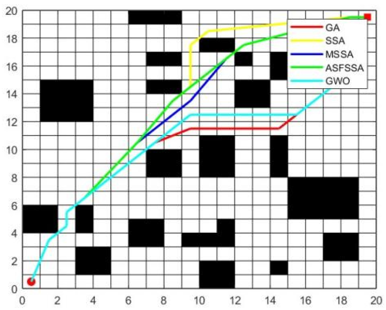
| Metrics | GA | SSA | MSSA | ASFSSA | GWO |
|---|---|---|---|---|---|
| Best | 28.0192 | 28.5777 | 28.5777 | 28.4193 | 28.4193 |
| Mean | 29.3141 | 29.9852 | 28.8836 | 28.5875 | 29.3287 |
| Worse | 30.4869 | 31.1395 | 29.7765 | 28.6315 | 30.8721 |
| Contribution | Description |
|---|---|
| Enhancement of Population Diversity | Introduced Latin Hypercube Sampling (LHS) during the initialization phase to enhance population diversity and avoid premature convergence. |
| Adaptive Weighting Mechanism | Applied an adaptive weighting mechanism to improve search efficiency, ensuring optimal performance at different stages of the search process. |
| Enhanced Global Search Capability | Utilized Cauchy mutation and cat disturbance strategies during the discovery phase to strengthen global search ability and prevent premature convergence to local optima. |
| Optimization Performance Validation | To verify the optimization performance and global optimization ability of the Modified Sparrow Search Algorithm (MSSA), tests were conducted on 23 benchmark functions, 10 CEC2019 test functions, and 100 five-dimensional GKLS test functions. |
| Stability and Precision | Experimental results indicate that MSSA outperforms other algorithms in terms of convergence precision and stability on most test functions. |
| Application to Real-World Problems | Demonstrated the effectiveness of MSSA by applying it to three real-world engineering problems, and a 20 × 20 robot path-planning problem further validating the improvements made. |
| Statistical Tests | Wilcoxon signed-rank test showed significant differences between MSSA and other algorithms at a 0.05 significance level. |
Disclaimer/Publisher’s Note: The statements, opinions and data contained in all publications are solely those of the individual author(s) and contributor(s) and not of MDPI and/or the editor(s). MDPI and/or the editor(s) disclaim responsibility for any injury to people or property resulting from any ideas, methods, instructions or products referred to in the content. |
© 2025 by the authors. Licensee MDPI, Basel, Switzerland. This article is an open access article distributed under the terms and conditions of the Creative Commons Attribution (CC BY) license (https://creativecommons.org/licenses/by/4.0/).
Share and Cite
Ma, Y.; Meng, W.; Wang, X.; Gu, P.; Zhang, X. Modified Sparrow Search Algorithm by Incorporating Multi-Strategy for Solving Mathematical Optimization Problems. Biomimetics 2025, 10, 299. https://doi.org/10.3390/biomimetics10050299
Ma Y, Meng W, Wang X, Gu P, Zhang X. Modified Sparrow Search Algorithm by Incorporating Multi-Strategy for Solving Mathematical Optimization Problems. Biomimetics. 2025; 10(5):299. https://doi.org/10.3390/biomimetics10050299
Chicago/Turabian StyleMa, Yunpeng, Wanting Meng, Xiaolu Wang, Peng Gu, and Xinxin Zhang. 2025. "Modified Sparrow Search Algorithm by Incorporating Multi-Strategy for Solving Mathematical Optimization Problems" Biomimetics 10, no. 5: 299. https://doi.org/10.3390/biomimetics10050299
APA StyleMa, Y., Meng, W., Wang, X., Gu, P., & Zhang, X. (2025). Modified Sparrow Search Algorithm by Incorporating Multi-Strategy for Solving Mathematical Optimization Problems. Biomimetics, 10(5), 299. https://doi.org/10.3390/biomimetics10050299