
UAV Path Planning: A Dual-Population Cooperative Honey Badger Algorithm for Staged Fusion of Multiple Differential Evolutionary Strategies

Abstract
1. Introduction
- Effective fusion of the randomized perturbation strategy in the whale algorithm and the honey badger algorithm.
- Proposing a staged two-population coevolutionary strategy that incorporates multiple differential variation approaches.
- Proposing an improved HBA algorithm (LRMHBA) that combines Latin hypercubic sampling with an elite strategy, a randomized perturbation strategy, and a staged two-population co-evolutionary strategy that fuses multiple differential variability approaches.
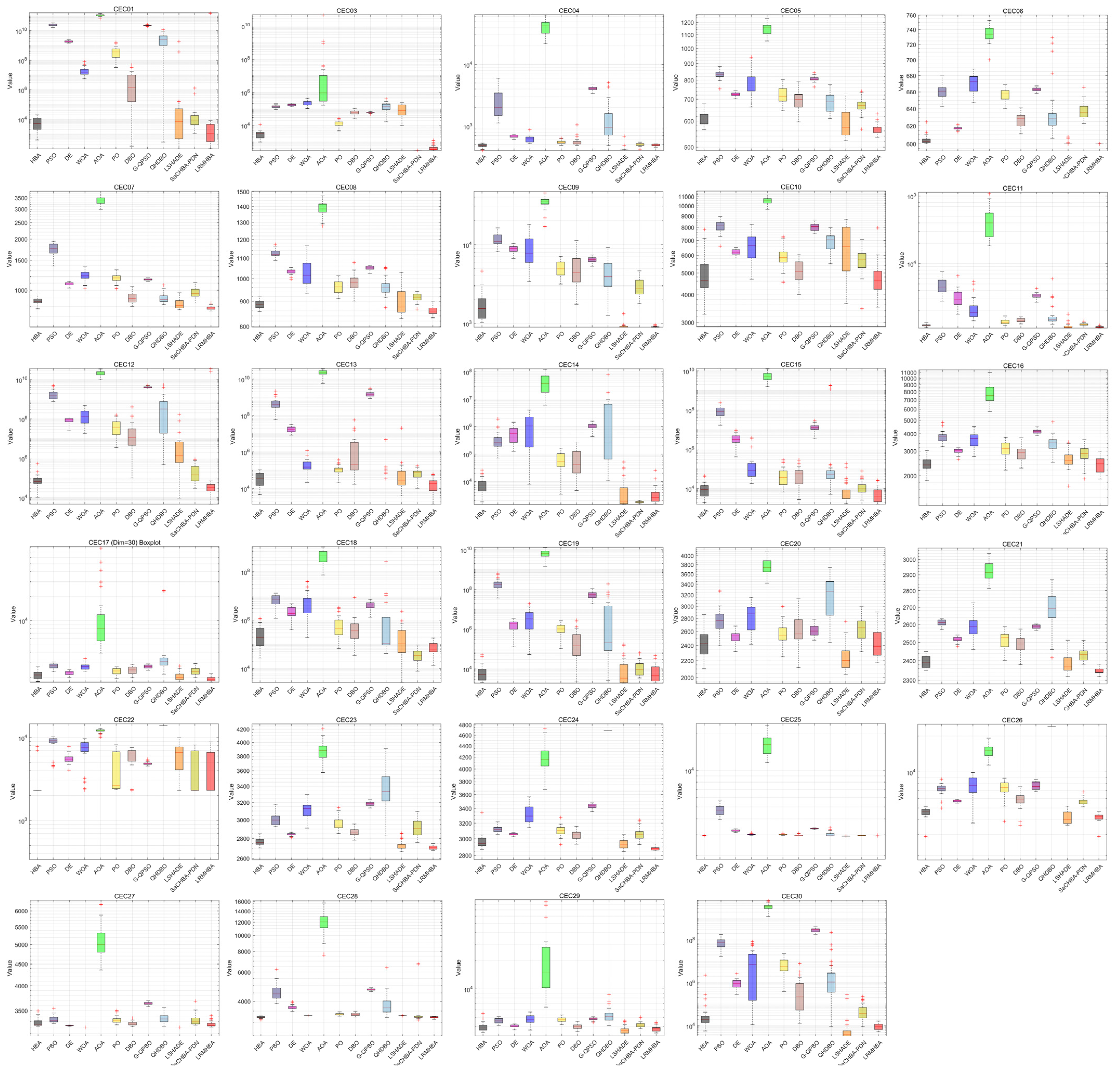
- Comparative performance tests were conducted on the LRMHBA algorithm against various competing algorithms, including highly referenced algorithms and their variants, recently developed high-performance algorithms, the champion algorithm, as well as the original HBA and its variant, using the CEC2017 test suite, with evaluations covering both low-dimensional (30-dimensional) and high-dimensional (100-dimensional) function optimization. Statistical analyses, including the Wilcoxon rank-sum test and Friedman test, along with ablation and exploration-exploitation experiments, were performed to validate the advancements of LRMHBA.
- The UAV flight cost is defined and three UAV 3D simulation scenarios from simple to complex are established, and the performance of path planning for each scenario is compared and analyzed with the LRMHBA algorithm and other competing algorithms, and the outcomes demonstrate the superiority of the LRMHBA method in the UAV path planning problem as well.
2. UAV Path Planning Modeling
2.1. Environmental Modeling
2.1.1. Base Terrain Model
2.1.2. Mountain Model
2.2. Operational Constraints
2.2.1. Flight Distance Cost
2.2.2. Flight Altitude Cost
2.2.3. Turning Maneuver Cost
2.2.4. Terrain Clearance Constraint
2.2.5. Obstacle Threat Cost
3. Honey Badger Algorithm (HBA)
3.1. Population Initialization
3.2. Excavation Phase
3.3. Honey Harvesting Phase
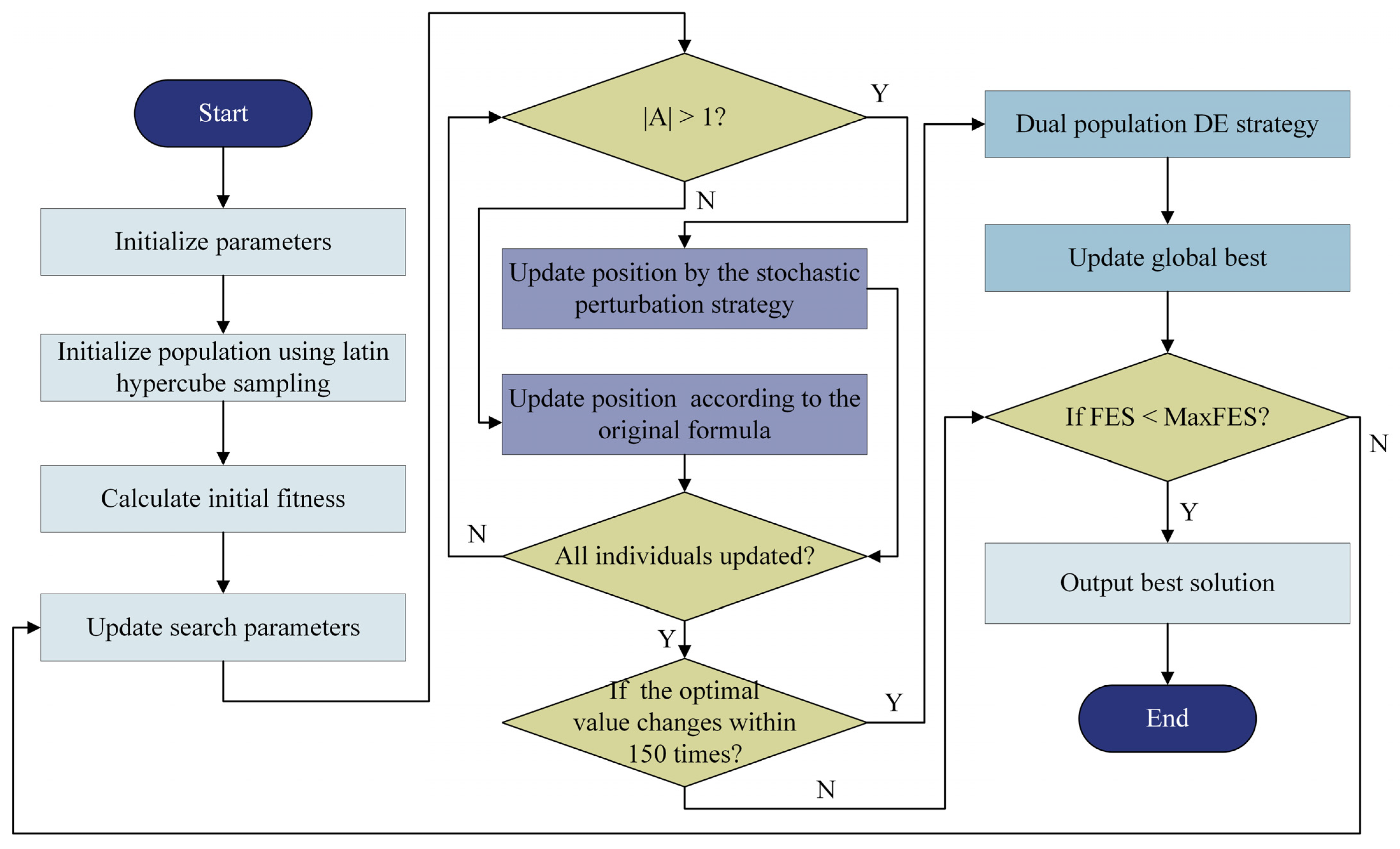
4. LRMHBA Algorithm
4.1. Hybrid LHS Initialization and Elite Guidance
- Generate N samples using LHS for uniform spatial coverage.
- Create another N sample through random sampling.
- Select the top N individuals by fitness ranking from the combined pool.
- Extract the elite 20% individuals to guide the proposed dual-population framework.

4.2. Stochastic Perturbation Strategy
Premature Convergence Analysis
4.3. The Staged Dual-Population Co-Evolutionary Strategy Integrating Multiple Differential Evolution Variants
4.3.1. Motivation and Framework
4.3.2. DE Mutation Operators
4.3.3. Dual-Population Mutation Method with Elite Individuals
- Group A (Top 50% fitness): Focused on precision exploitation.
- Group B (Bottom 50% fitness): Dedicated to spatial exploration.
- 1.
- Phase I (Initial 2/3 iterations): Exploration Emphasis.
- Group A: DE/mean-current/2.
- Group B: DE/rand/1.
- 2.
- Phase II (Final 1/3 iterations): Exploitation Emphasis.
- Group A: DE/current-to-best/2.
- Group B: DE/mean-current/2.
4.4. Pseudocode and Flowchart of LRMHBA
| Algorithm 1 Pseudocode of LRMHBA |
| 1: Initialize population X using Latin hypercube sampling and elite strategy do using Equations (17), (20), (23) and (24). do then 6: Update position using random individual using Equations (25) and (26). 7: else using Equations (16) and (22). 9: end if 10: Update if better solution found. 11: end for and no improvement in last 150 evaluations then then 14: Set population ratios: 0% mean-current/2, 50% current-to-best/2, 50% rand/1 15: else 16: Set population ratios: 50% mean-current/2, 50% current-to-best/2, 0% rand/1 17: end if 18: Sort population by fitness and divide into groups 19: for each group do 20: if Group 1 (mean-current/2) then 21: Apply mutation using Equation (33). 22: else if Group 2 (current-to-best/2) then 23: Apply mutation using Equation (32). 24: else if Group 3 (rand/1) then 25: Apply mutation using Equation (28). 26: end if 27: Apply binomial crossover with probability. 28: Update if better solution found. 29: end for 30: end if 31: Update X_prey and Food_Score if better solution found. 32: end while 33: Return Food_Score, X_prey. |
4.5. Time Complexity Analysis
- Latin hypercube sampling during initialization:
- Elite strategy sorting in the initialization phase:
- Stochastic perturbation strategy:
- Dual-population mutation method:
5. Algorithm Performance Testing and Analysis
- Champion algorithm: LSHADE [59];
- HBA algorithm and its variant: HBA, SaCHBA_PDN.
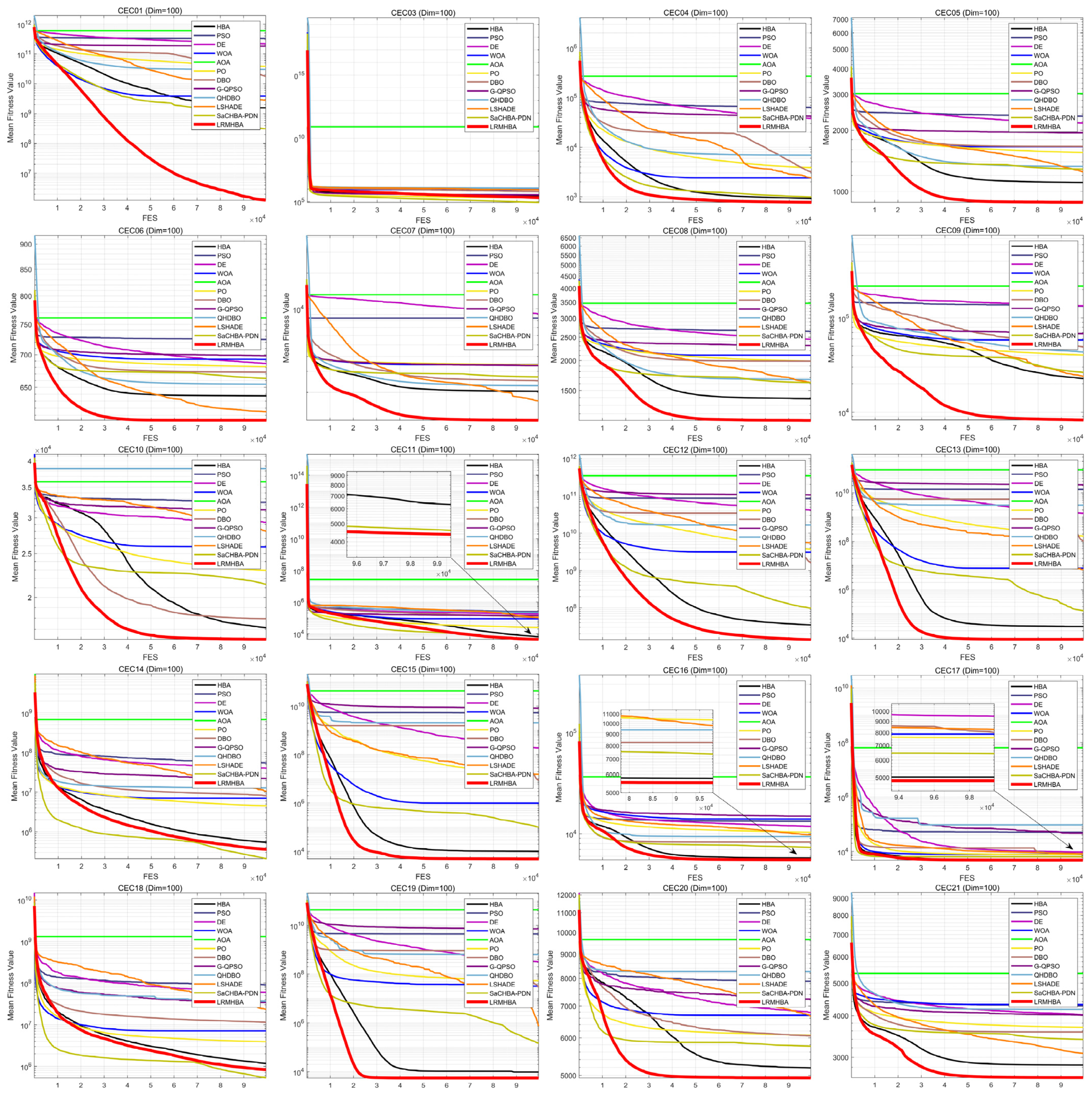
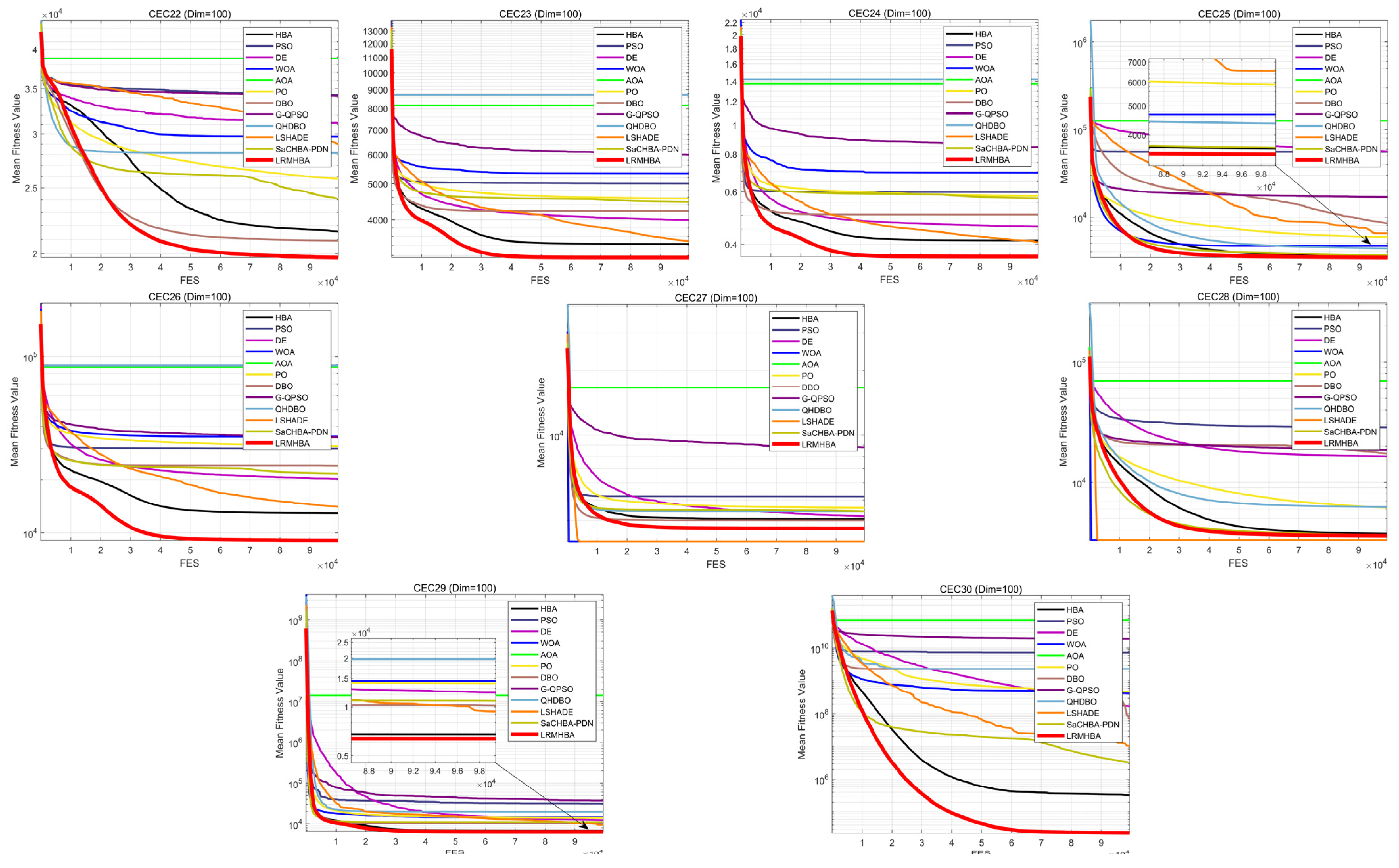
5.1. Results Analysis on CEC2017
5.2. Ablation Study
- LRMHBA1: HBA combined with Latin hypercube sampling and elite strategy.
- LRMHBA2: HBA combined with a random disturbance strategy.
- LRMHBA3: HBA combined with a staged dual-population co-evolutionary strategy integrating multiple differential evolution variants.
5.3. Exploration and Exploitation Experiment
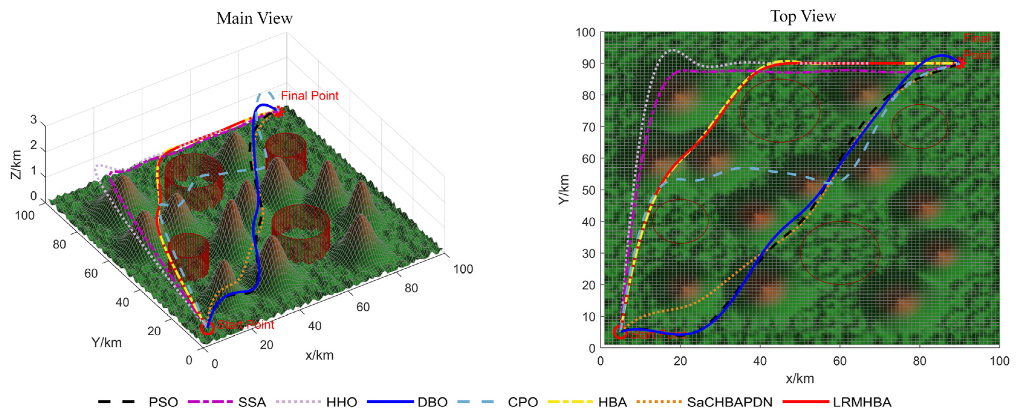
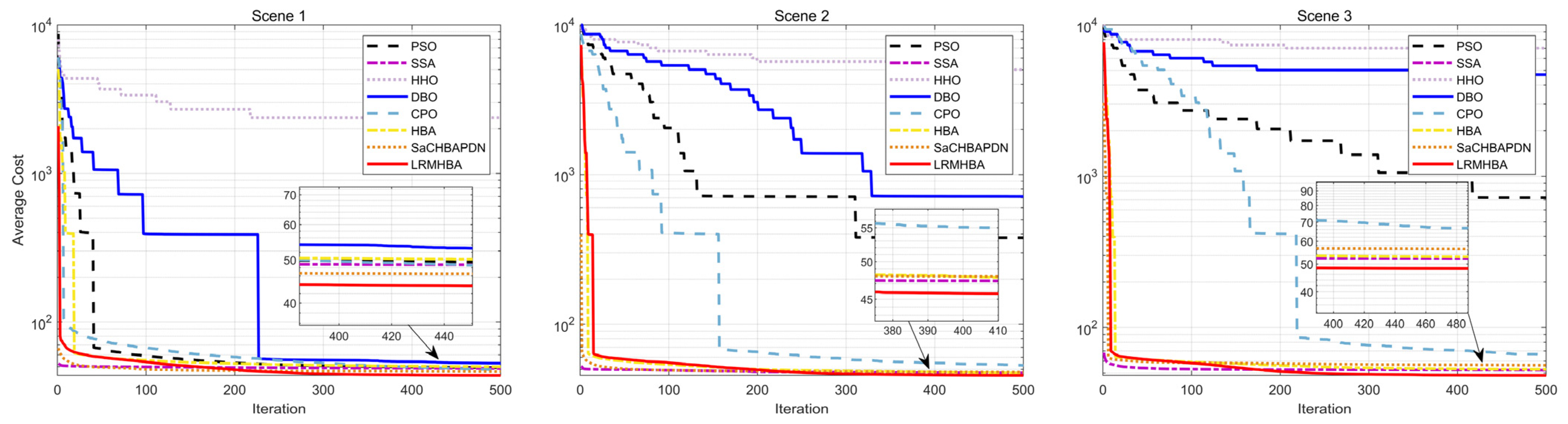
6. UAV Path Planning Simulation Experiments
6.1. Experimental Setup
6.2. Analysis of Experimental Results
7. Conclusions
Author Contributions
Funding
Institutional Review Board Statement
Data Availability Statement
Conflicts of Interest
Appendix A

| No. | Functions | ||
|---|---|---|---|
| Unimodal Functions | 1 | Shifted and Rotated Bent Cigar Function | 100 |
| 3 | Shifted and Rotated Zakharov Function | 200 | |
| Simple Multimodal Functions | 4 | Shifted and Rotated Rosenbrock’s Function | 300 |
| 5 | Shifted and Rotated Rastrigin’s Function | 400 | |
| 6 | Shifted and Rotated Expanded Scaffer’s F6 Function | 500 | |
| 7 | Shifted and Rotated Lunacek Bi_Rastrigin Function | 600 | |
| 8 | Shifted and Rotated Non-Continuous Rastrigin’s Function | 700 | |
| 9 | Shifted and Rotated Levy Function | 800 | |
| 10 | Shifted and Rotated Schwefel’s Function | 900 | |
| Hybrid Functions | 11 | Hybrid Function 1 (N = 3) | 1000 |
| 12 | Hybrid Function 2(N = 3) | 1100 | |
| 13 | Hybrid Function 3 (N = 3) | 1200 | |
| 14 | Hybrid Function 4 (N = 4) | 1300 | |
| 15 | Hybrid Function 5 (N = 4) | 1400 | |
| 16 | Hybrid Function 6 (N = 4) | 1500 | |
| 17 | Hybrid Function 6 (N = 5) | 1600 | |
| 18 | Hybrid Function 6 (N = 5) | 1700 | |
| 19 | Hybrid Function 6 (N = 5) | 1800 | |
| 20 | Hybrid Function 6 (N = 6) | 1900 | |
| Composition Functions | 21 | Composition Function 1 (N = 3) | 2000 |
| 22 | Composition Function 2 (N = 3) | 2100 | |
| 23 | Composition Function 3 (N = 4) | 2200 | |
| 24 | Composition Function 4 (N = 4) | 2300 | |
| 25 | Composition Function 5 (N = 5) | 2400 | |
| 26 | Composition Function 6 (N = 5) | 2500 | |
| 27 | Composition Function 7 (N = 6) | 2600 | |
| 28 | Composition Function 8 (N = 6) | 2700 | |
| 29 | Composition Function 9 (N = 3) | 2800 | |
| 30 | Composition Function 10 (N = 3) | 2900 | |
References
- Alejandro, P.; Daniel, R.; Alejandro, P.; Enrique, F. A review of artificial intelligence applied to path planning in UAV swarms. Neural Comput. Appl. 2022, 34, 153–170. [Google Scholar] [CrossRef]
- Jones, M.; Soufiene, D.; Kristopher, W. Path-planning for unmanned aerial vehicles with environment complexity considerations: A survey. ACM Comput. Surv. 2023, 55, 1–39. [Google Scholar] [CrossRef]
- Hart, P.; Nils, J.; Bertram, R. A formal basis for the heuristic determination of minimum cost paths. IEEE Trans. Syst. Sci. Cybern. 1968, 4, 100–107. [Google Scholar] [CrossRef]
- Khatib, O. Real-time obstacle avoidance for manipulators and mobile robots. Int. J. Robot. Res. 1986, 5, 90–98. [Google Scholar] [CrossRef]
- Nasir, J.; Islam, F.; Ayaz, Y. Adaptive Rapidly-Exploring-Random-Tree-Star (RRT*)-Smart: Algorithm Characteristics and Behavior Analysis in Complex Environments. Asia-Pac. J. Inf. Technol. Multimed 2013, 2, 39–51. [Google Scholar] [CrossRef]
- Desale, S.; Rasool, A.; Andhale, S.; Rane, P. Heuristic and meta-heuristic algorithms and their relevance to the real world: A survey. Int. J. Comput. Eng. Res. Trends 2015, 2, 296–304. [Google Scholar]
- Sadeghian, Z.; Akbari, E.; Nematzadeh, H.; Motameni, H. A review of feature selection methods based on meta-heuristic algorithms. J. Exp. Theor. Artif. Intell. 2025, 37, 1–51. [Google Scholar] [CrossRef]
- Hashim, F.A.; Mostafa, R.R.; Hussien, A.G.; Mirjalili, S.; Sallam, K.M. Fick’s Law Algorithm: A physical law-based algorithm for numerical optimization. Knowl.-Based Syst. 2023, 260, 110146. [Google Scholar] [CrossRef]
- Hu, G.; Cheng, M.; Houssein, E.H.; Hussien, A.G.; Abualigah, L. SDO: A novel sled dog-inspired optimizer for solving engineering problems. Adv. Eng. Inform. 2024, 62, 102783. [Google Scholar] [CrossRef]
- Kennedy, J.; Russell, E. Particle swarm optimization. In Proceedings of the ICNN’95-International Conference on Neural Networks, Perth, WA, Australia, 27 November–1 December 1995. [Google Scholar] [CrossRef]
- Karaboga, D.; Bahriye, B. A powerful and efficient algorithm for numerical function optimization: Artificial bee colony (ABC) algorithm. J. Glob. Optim. 2007, 39, 459–471. [Google Scholar] [CrossRef]
- Mirjalili, S.; Andrew, L. The whale optimization algorithm. Adv. Eng. Softw. 2016, 95, 51–67. [Google Scholar] [CrossRef]
- Heidari, A.; Mirjalili, S.; Faris, H.; Aljarah, I.; Mafarja, M.; Chen, H. Harris hawks optimization: Algorithm and applications. Future Gener. Comput. Syst. 2019, 97, 849–872. [Google Scholar] [CrossRef]
- Xue, J.; Shen, B. A novel swarm intelligence optimization approach: Sparrow search algorithm. Syst. Sci. Control Eng. 2020, 8, 22–34. [Google Scholar] [CrossRef]
- Xue, J.; Shen, B. Dung beetle optimizer: A new meta-heuristic algorithm for global optimization. J. Supercomput. 2023, 79, 7305–7336. [Google Scholar] [CrossRef]
- Abdel, B.; Mohamed, R.; Mohamed, A. Crested Porcupine Optimizer: A new nature-inspired metaheuristic. Knowl.-Based Syst. 2024, 284, 111257. [Google Scholar] [CrossRef]
- Li, Y.; Zhang, L.; Cai, B.; Liang, Y. Unified path planning for composite UAVs via Fermat point-based grouping particle swarm optimization. Aerosp. Sci. Technol. 2024, 148, 109088. [Google Scholar] [CrossRef]
- Han, Z.; Chen, M.; Shao, S.; Wu, Q. Improved artificial bee colony algorithm-based path planning of unmanned autonomous helicopter using mul-ti-strategy evolutionary learning. Aerosp. Sci. Technol. 2022, 122, 107374. [Google Scholar] [CrossRef]
- Dai, Y.; Yu, J.; Zhang, C.; Zhan, B.; Zheng, X. A novel whale optimization algorithm of path planning strategy for mobile robots. Appl. Intell. 2023, 53, 10843–10857. [Google Scholar] [CrossRef]
- Tang, C.; Li, W.; Han, T.; Yu, L.; Cui, T. Multi-Strategy Improved Harris Hawk Optimization Algorithm and Its Application in Path Planning. Biomimetics 2024, 9, 552. [Google Scholar] [CrossRef]
- Cheng, L.; Ling, G.; Liu, F.; Ge, M. Application of uniform experimental design theory to multi-strategy improved sparrow search algorithm for UAV path planning. Expert Syst. Appl. 2024, 255, 124849. [Google Scholar] [CrossRef]
- Chen, Q.; Wang, Y.; Sun, Y. An improved dung beetle optimizer for UAV 3D path planning. J. Supercomput. 2024, 80, 26537–26567. [Google Scholar] [CrossRef]
- Liu, S.; Jin, Z.; Lin, H.; Lu, H. An improve crested porcupine algorithm for UAV delivery path planning in challenging environments. Sci. Rep. 2024, 14, 20445. [Google Scholar] [CrossRef] [PubMed]
- Hashim, F.; Houssein, E.; Hussain, K.; Mabrouk, M.; Al-Atabany, W. Honey Badger Algorithm: New metaheuristic algorithm for solving optimization problems. Math. Comput. Simul. 2022, 192, 84–110. [Google Scholar] [CrossRef]
- Abasi, A.K.; Aloqaily, M.; Guizani, M. Optimization of cnn using modified honey badger algorithm for sleep apnea detection. Expert Syst. Appl. 2023, 229, 120484. [Google Scholar] [CrossRef]
- Nassef, A.; Houssein, E.; Helmy, B.; Rezk, H. Modified honey badger algorithm based global MPPT for triple-junction solar photovoltaic system under partial shading condition and global optimization. Energy 2022, 254, 124363. [Google Scholar] [CrossRef]
- Dao, T.; Nguyen, T.; Nguyen, V. An improved honey badger algorithm for coverage optimization in wireless sensor network. J. Internet Technol. 2023, 24, 363–377. [Google Scholar]
- Houssein, E.; Emam, M.; Singh, N.; Samee, N.; Alabdulhafith, M.; Çelik, E. An improved honey badger algorithm for global optimization and multilevel thresholding segmentation: Real case with brain tumor images. Clust. Comput. 2024, 27, 14315–14364. [Google Scholar] [CrossRef]
- Jain, D.; Weiping, D.; Ketan, K. Training fuzzy deep neural network with honey badger algorithm for intrusion detection in cloud environment. Int. J. Mach. Learn. Cybern. 2023, 14, 2221–2237. [Google Scholar] [CrossRef]
- Xu, Y.; Zhong, R.; Cao, Y.; Zhang, C.; Yu, J. Symbiotic mechanism-based honey badger algorithm for continuous optimization. Clust. Comput. 2025, 28, 133. [Google Scholar] [CrossRef]
- Düzenlí, T.; Funda, K.; Salih, B.; Aydemir, S.B. Improved honey badger algorithms for parameter extraction in photovoltaic models. Optik 2022, 268, 169731. [Google Scholar] [CrossRef]
- Bansal, B.; Sahoo, A. Enhanced honey badger algorithm for multi-view subspace clustering based on consensus representation. Soft Comput. 2024, 28, 13307–13329. [Google Scholar] [CrossRef]
- Hu, G.; Zhong, J.; Guo, W. SaCHBA_PDN: Modified honey badger algorithm with multi-strategy for UAV path planning. Expert Syst. Appl. 2023, 223, 119941. [Google Scholar] [CrossRef]
- Zhang, X.; Duan, H. An improved constrained differential evolution algorithm for unmanned aerial vehicle global route planning. Appl. Soft Comput. 2015, 26, 270–284. [Google Scholar] [CrossRef]
- Service, T. A No Free Lunch theorem for multi-objective optimization. Inf. Process. Lett. 2010, 110, 917–923. [Google Scholar] [CrossRef]
- Abasi, A.K.; Aloqaily, M.; Guizani, M. Bare-bones based honey badger algorithm of CNN for Sleep Apnea detection. Clust. Comput. 2024, 27, 6145–6165. [Google Scholar] [CrossRef]
- Fathy, A.; Rezk, H.; Ferahtia, S.; Ghoniem, R.; Alkanhel, R. An efficient honey badger algorithm for scheduling the microgrid energy management. Energy Rep. 2023, 9, 2058–2074. [Google Scholar] [CrossRef]
- Han, E.; Noradin, G. Model identification of proton-exchange membrane fuel cells based on a hybrid convolutional neural network and extreme learning machine optimized by improved honey badger algorithm. Sustain. Energy Technol. Assess. 2022, 52, 102005. [Google Scholar] [CrossRef]
- Tan, Y.; Liu, S.; Zhang, L.; Song, J.; Ren, Y. The Application of an Improved LESS Dung Beetle Optimization in the Intelligent Topological Reconfiguration of ShipPower Systems. J. Mar. Sci. Eng. 2024, 12, 1843. [Google Scholar] [CrossRef]
- Wang, K.; Si, P.; Chen, L.; Li, Z. 3D Path Planning of Unmanned Aerial Vehicle Based on Enhanced Sand Cat Swarm Optimization Algorithm. Acta Armamentarii 2023, 44, 3382–3393. [Google Scholar]
- Ning, Y.; Zheng, B.; Long, Z.; Luo, J. Complex 3D Path Planning for UAVs Based on CMPSO Algorithm. Electron. Opt. Control 2024, 31, 35–42. [Google Scholar]
- Luo, J.; Tian, Y.; Wang, Z. Research on Unmanned Aerial Vehicle Path Planning. Drones 2024, 8, 51. [Google Scholar] [CrossRef]
- Zhou, X.; Tang, Z.; Wang, N.; Yang, C.; Huang, T. A novel state transition algorithm with adaptive fuzzy penalty for multi-constraint UAV path planning. Expert Syst. Appl. 2024, 248, 123481. [Google Scholar] [CrossRef]
- Michael, D. Latin hypercube sampling as a tool in uncertainty analysis of computer models. In Proceedings of the 24th Conference on Winter Simulation, Arlington, VA, USA, 13–16 December 1992. [Google Scholar]
- Stein, M. Large sample properties of simulations using Latin hypercube sampling. Technometrics 1987, 29, 143–151. [Google Scholar] [CrossRef]
- Storn, R. On the usage of differential evolution for function optimization. In Proceedings of the North American Fuzzy Information Processing, Berkeley, CA, USA, 19–22 June 1996. [Google Scholar] [CrossRef]
- Storn, R.; Price, K. Differential evolution–a simple and efficient heuristic for global optimization over continuous spaces. J. Glob. Optim. 1997, 11, 341–359. [Google Scholar] [CrossRef]
- Gämperle, R.; Sibylle, D.; Petros, K. A parameter study for differential evolution. Adv. Intell. Syst. Fuzzy Syst. Evol. Comput. 2002, 10, 293–298. [Google Scholar]
- Yu, W.; Shen, M.; Chen, W.; Zhan, Z.; Gong, Y.; Lin, Y.; Zhang, J. Differential evolution with two-level parameter adaptation. IEEE Trans. Cybern. 2013, 44, 1080–1099. [Google Scholar] [CrossRef]
- Li, Y.; Wang, S.; Yang, B. An improved differential evolution algorithm with dual mutation strategies collaboration. Expert Syst. Appl. 2020, 153, 113451. [Google Scholar] [CrossRef]
- Zuo, M.; Guo, C. DE/current−to−better/1: A new mutation operator to keep population diversity. Intell. Syst. Appl. 2022, 14, 200063. [Google Scholar] [CrossRef]
- Rauf, H.; Gao, J.; Almadhor, A.; Haider, A.; Zhang, Y.; Al-Turjman, F. Multi population-based chaotic differential evolution for multi-modal and multi-objective optimization problems. Appl. Soft Comput. 2023, 132, 109909. [Google Scholar] [CrossRef]
- Layeb, A. Differential evolution algorithms with novel mutations, adaptive parameters, and Weibull flight operator. Soft Comput. 2024, 28, 7039–7091. [Google Scholar] [CrossRef]
- Price, K. Multi population-based chaotic differential evolution for multi-modal and multi-objective optimization problems. In Proceedings of the North American Fuzzy Information Processing, Berkeley, CA, USA, 19–22 June 1996. [Google Scholar] [CrossRef]
- Abualigah, L.; Diabat, A.; Mirjalili, S.; Abd Elaziz, M.; Gandomi, A. The arithmetic optimization algorithm. Comput. Methods Appl. Mech. Eng. 2021, 376, 113609. [Google Scholar] [CrossRef]
- dos Santos Coelho, L. Gaussian quantum-behaved particle swarm optimization approaches for constrained engineering design problems. Expert Syst. Appl. 2010, 37, 1676–1683. [Google Scholar] [CrossRef]
- Lian, J.; Hui, G.; Ma, L.; Zhu, T.; Wu, X.; Heidari, A.A.; Chen, Y.; Chen, H. Parrot optimizer: Algorithm and applications to medical problems. Comput. Biol. Med. 2024, 172, 108064. [Google Scholar] [CrossRef] [PubMed]
- Zhu, F.; Li, G.; Tang, H.; Li, Y.; Lv, X.; Wang, X. Dung beetle optimization algorithm based on quantum computing and multi-strategy fusion for solving engineering problems. Expert Syst. Appl. 2024, 236, 121219. [Google Scholar] [CrossRef]
- Tanabe, R.; Fukunaga, A.S. Improving the search performance of SHADE using linear population size reduction. In Proceedings of the 2014 IEEE Congress on Evolutionary Computation (CEC), Beijing, China, 6–11 July 2014. [Google Scholar] [CrossRef]
- Zhu, F.; Li, G.; Tang, H.; Li, Y.; Lv, X.; Wang, X. Population diversity maintenance in brain storm optimization algorithm. J. Artif. Intell. Soft Comput. Res. 2014, 4, 83–97. [Google Scholar] [CrossRef]
- Morales-Castañeda, B.; Zaldivar, D.; Cuevas, E.; Fausto, F.; Rodríguez, A. A better balance in metaheuristic algorithms: Does it exist? Swarm Evol. Comput. 2020, 54, 100671. [Google Scholar] [CrossRef]


| Methods | Applications | Authors |
|---|---|---|
| Combined quasi-location learning, arbitrarily weighted agents, and adaptive mutation methods. | Selected optimal hyperparameter values for a convolutional neural network CNN applied to sleep apnea diagnosis. | Abasi et al. [25] |
| Proposed an efficient local search method, called dimensional learning hunting (DLH). | Identified the peak of the global maximum output power of PV cells. | Nassef et al. [26] |
| Combined HBA with elite backward learning and multidirectional strategies. | Wireless sensor network coverage problem. | Dao et al. [27] |
| Implemented an Enhanced Solution Quality (ESQ) approach. | Biomedical image segmentation. | Houssei et al. [28] |
| Developed a new fuzzy deep neural network (FDNN) combined with HBA. | Cloud Computing Privacy Protection Intrusion Detection. | Jain et al. [29] |
| Proposed a symbiosis-based HBA (SHBA) in conjunction with the cooperative symbio-sis mechanism between honey badgers and honeycreepers. | Engineering problems | Xu et al. [30] |
| Hybridization of Contrastive Learning with the Honey Badger Algorithm. | Optimization of solar system model parameter values. | Düzenlí et al. [31] |
| Designed a sparse jNMF method framework guided by the Enhanced Honey Badger Algorithm (EHBA) | Integrated clustering problem | Bansal et al. [32] |
| Algorithms | Parameters | Setting Value |
|---|---|---|
| HBA | (the ability of a honey badger to get food) | 6 |
| 2 | ||
| PSO | Cognitive and social factors | |
| DE | Crossover rate | |
| Scaling factor | ||
| WOA | Fluctuation range | Linear decrease from 2 to 0 |
| AOA | Control parameter | |
| Sensitive parameter | ||
| DBO | Disruption factor | |
| Luminous efficacy | ||
| sensitivity parameter | ||
| GQPSO | Inertia weight | Linear decrease from 1 to 0.5 |
| Cognitive and social factors | ||
| QHDBO | Disruption factor | |
| Luminous efficacy | ||
| sensitivity parameter | ||
| LSHADE | Crossover rate | |
| Scaling factor | ||
| SaCHBA_PDN | ||
| LRMHBA | Scaling factor | |
| Crossover rate | ||
| 6 | ||
| 2 |
| Function | Index | HBA | PSO | DE | WOA | AOA | PO | DBO | GQPSO | QHDBO | LSHADE | SaCHBA_PDN | LRMHBA |
|---|---|---|---|---|---|---|---|---|---|---|---|---|---|
| CEC01 | Best | 1.338 × 10+2 | 1.450 × 10+10 | 1.524 × 10+9 | 6.486 × 10+6 | 8.346 × 10+10 | 6.412 × 10+6 | 1.057 × 10+2 | 1.853 × 10+10 | 4.951 × 10+2 | 1.017 × 10+2 | 1.039 × 10+3 | 1.000 × 10+2 |
| Mean | 5.527 × 10+3 | 2.331 × 10+10 | 1.939 × 10+9 | 2.233 × 10+7 | 1.142 × 10+11 | 2.762 × 10+8 | 8.235 × 10+6 | 2.288 × 10+10 | 3.387 × 10+9 | 6.204 × 10+6 | 6.094 × 10+5 | 3.652 × 10+9 | |
| Std | 5.349 × 10+3 | 4.676 × 10+9 | 1.954 × 10+8 | 1.900 × 10+7 | 1.372 × 10+10 | 3.256 × 10+8 | 1.813 × 10+7 | 1.635 × 10+9 | 3.536 × 10+9 | 2.818 × 10+7 | 1.801 × 10+6 | 2.000 × 10+10 | |
| Rank | 2 | 11 | 9 | 6 | 12 | 7 | 5 | 10 | 8 | 3 | 4 | 1 | |
| CEC03 | Best | 8.876 × 10+2 | 9.232 × 10+4 | 1.096 × 10+5 | 7.498 × 10+4 | 1.849 × 10+5 | 5.820 × 10+3 | 2.776 × 10+4 | 5.180 × 10+4 | 3.618 × 10+4 | 6.933 × 10+3 | 3.000 × 10+2 | 3.000 × 10+2 |
| Mean | 3.116 × 10+3 | 1.384 × 10+5 | 1.687 × 10+5 | 2.196 × 10+5 | 2.536 × 10+8 | 1.470 × 10+4 | 5.913 × 10+4 | 6.176 × 10+4 | 1.809 × 10+5 | 9.158 × 10+4 | 3.017 × 10+2 | 7.527 × 10+2 | |
| Std | 1.773 × 10+3 | 2.807 × 10+4 | 2.485 × 10+4 | 7.259 × 10+4 | 1.199 × 10+9 | 5.493 × 10+3 | 1.606 × 10+4 | 3.754 × 10+3 | 1.103 × 10+5 | 8.858 × 10+4 | 3.516 × 10+0 | 8.211 × 10+2 | |
| Rank | 3 | 8 | 10 | 11 | 12 | 4 | 5 | 6 | 9 | 7 | 1 | 2 | |
| CEC04 | Best | 4.600 × 10+2 | 1.171 × 10+3 | 6.183 × 10+2 | 4.808 × 10+2 | 1.267 × 10+4 | 4.849 × 10+2 | 4.769 × 10+2 | 2.829 × 10+3 | 4.968 × 10+2 | 4.251 × 10+2 | 4.043 × 10+2 | 4.681 × 10+2 |
| Mean | 4.894 × 10+2 | 2.252 × 10+3 | 6.975 × 10+2 | 5.945 × 10+2 | 4.428 × 10+4 | 5.443 × 10+2 | 5.507 × 10+2 | 4.025 × 10+3 | 9.799 × 10+2 | 4.286 × 10+2 | 5.154 × 10+2 | 4.923 × 10+2 | |
| Std | 1.833 × 10+1 | 8.389 × 10+2 | 3.770 × 10+1 | 5.832 × 10+1 | 1.042 × 10+4 | 3.439 × 10+1 | 7.827 × 10+1 | 4.283 × 10+2 | 5.387 × 10+2 | 6.277 × 10+0 | 5.107 × 10+1 | 1.530 × 10+1 | |
| Rank | 2 | 10 | 9 | 7 | 12 | 6 | 5 | 11 | 8 | 1 | 4 | 3 | |
| CEC05 | Best | 5.468 × 10+2 | 7.946 × 10+2 | 6.984 × 10+2 | 6.640 × 10+2 | 1.035 × 10+3 | 6.367 × 10+2 | 6.169 × 10+2 | 7.828 × 10+2 | 6.103 × 10+2 | 5.249 × 10+2 | 6.135 × 10+2 | 5.298 × 10+2 |
| Mean | 6.026 × 10+2 | 8.279 × 10+2 | 7.280 × 10+2 | 7.949 × 10+2 | 1.154 × 10+3 | 7.340 × 10+2 | 7.023 × 10+2 | 8.075 × 10+2 | 6.969 × 10+2 | 6.002 × 10+2 | 6.567 × 10+2 | 5.646 × 10+2 | |
| Std | 2.090 × 10+1 | 1.946 × 10+1 | 1.121 × 10+1 | 6.350 × 10+1 | 4.378 × 10+1 | 4.108 × 10+1 | 5.524 × 10+1 | 1.277 × 10+1 | 5.881 × 10+1 | 5.491 × 10+1 | 2.701 × 10+1 | 1.841 × 10+1 | |
| Rank | 3 | 11 | 7 | 9 | 12 | 8 | 6 | 10 | 5 | 2 | 4 | 1 | |
| CEC06 | Best | 6.004 × 10+2 | 6.465 × 10+2 | 6.135 × 10+2 | 6.456 × 10+2 | 7.128 × 10+2 | 6.369 × 10+2 | 6.092 × 10+2 | 6.570 × 10+2 | 6.154 × 10+2 | 6.000 × 10+2 | 6.139 × 10+2 | 6.000 × 10+2 |
| Mean | 6.051 × 10+2 | 6.623 × 10+2 | 6.185 × 10+2 | 6.710 × 10+2 | 7.351 × 10+2 | 6.557 × 10+2 | 6.287 × 10+2 | 6.631 × 10+2 | 6.351 × 10+2 | 6.002 × 10+2 | 6.315 × 10+2 | 6.042 × 10+2 | |
| Std | 4.823 × 10+0 | 7.407 × 10+0 | 1.804 × 10+0 | 1.295 × 10+1 | 9.505 × 10+0 | 8.484 × 10+0 | 8.472 × 10+0 | 2.505 × 10+0 | 2.201 × 10+1 | 7.372 × 10⁻¹ | 7.130 × 100 | 2.317 × 10+1 | |
| Rank | 3 | 9 | 4 | 11 | 12 | 8 | 5 | 10 | 6 | 1 | 7 | 2 | |
| CEC07 | Best | 8.016 × 10+2 | 1.507 × 10+3 | 1.011 × 10+3 | 1.022 × 10+3 | 2.891 × 10+3 | 9.921 × 10+2 | 8.211 × 10+2 | 1.130 × 10+3 | 7.996 × 10+2 | 7.614 × 10+2 | 8.541 × 10+2 | 7.569 × 10+2 |
| Mean | 8.637 × 10+2 | 1.781 × 10+3 | 1.084 × 10+3 | 1.230 × 10+3 | 3.254 × 10+3 | 1.146 × 10+3 | 9.310 × 10+2 | 1.155 × 10+3 | 8.807 × 10+2 | 8.447 × 10+2 | 9.773 × 10+2 | 7.849 × 10+2 | |
| Std | 4.823 × 10+0 | 7.407 × 10+0 | 1.804 × 10+0 | 1.295 × 10+1 | 9.505 × 10+0 | 8.484 × 10+0 | 8.472 × 10+0 | 2.505 × 10+0 | 2.201 × 10+1 | 7.372 × 10⁻¹ | 7.130 × 10+0 | 2.317 × 10+1 | |
| Rank | 3 | 11 | 7 | 10 | 12 | 8 | 5 | 9 | 4 | 2 | 6 | 1 | |
| CEC08 | Best | 8.497 × 10+2 | 1.097 × 10+3 | 1.003 × 10+3 | 9.079 × 10+2 | 1.301 × 10+3 | 9.283 × 10+2 | 9.194 × 10+2 | 1.037 × 10+3 | 8.948 × 10+2 | 8.289 × 10+2 | 8.766 × 10+2 | 8.259 × 10+2 |
| Mean | 8.952 × 10+2 | 1.137 × 10+3 | 1.036 × 10+3 | 1.009 × 10+3 | 1.384 × 10+3 | 9.754 × 10+2 | 1.003 × 10+3 | 1.056 × 10+3 | 9.682 × 10+2 | 8.931 × 10+2 | 9.267 × 10+2 | 8.641 × 10+2 | |
| Std | 1.728 × 10+1 | 2.386 × 10+1 | 1.398 × 10+1 | 5.327 × 10+1 | 4.284 × 10+1 | 2.950 × 10+1 | 4.809 × 10+1 | 1.097 × 10+1 | 4.448 × 10+1 | 6.405 × 10+1 | 2.958 × 10+1 | 2.101 × 10+1 | |
| Rank | 2 | 11 | 9 | 7 | 12 | 6 | 8 | 10 | 5 | 3 | 4 | 1 | |
| CEC09 | Best | 1.321 × 10+3 | 7.533 × 10+3 | 6.338 × 10+3 | 5.233 × 10+3 | 1.936 × 10+4 | 2.744 × 10+3 | 1.501 × 10+3 | 5.443 × 10+3 | 1.680 × 10+3 | 9.000 × 10+2 | 1.713 × 10+3 | 9.001 × 10+2 |
| Mean | 1.926 × 10+3 | 1.121 × 10+4 | 8.499 × 10+3 | 8.871 × 10+3 | 3.443 × 10+4 | 5.213 × 10+3 | 5.083 × 10+3 | 6.333 × 10+3 | 4.394 × 10+3 | 9.826 × 10+2 | 3.040 × 10+3 | 9.135 × 10+2 | |
| Std | 5.932 × 10+2 | 2.369 × 10+3 | 9.801 × 10+2 | 3.239 × 10+3 | 5.488 × 10+3 | 1.076 × 10+3 | 2.136 × 10+3 | 4.551 × 10+2 | 1.989 × 10+3 | 2.910 × 10+2 | 9.291 × 10+2 | 3.453 × 10+1 | |
| Rank | 3 | 11 | 10 | 9 | 12 | 7 | 6 | 8 | 5 | 2 | 4 | 1 | |
| CEC10 | Best | 3.510 × 10+3 | 7.510 × 10+3 | 5.703 × 10+3 | 5.186 × 10+3 | 9.690 × 10+3 | 3.960 × 10+3 | 4.037 × 10+3 | 7.336 × 10+3 | 5.674 × 10+3 | 4.053 × 10+3 | 4.315 × 10+3 | 3.634 × 10+3 |
| Mean | 4.973 × 10+3 | 8.093 × 10+3 | 6.232 × 10+3 | 6.530 × 10+3 | 1.060 × 10+4 | 5.771 × 10+3 | 5.190 × 10+3 | 7.948 × 10+3 | 6.834 × 10+3 | 5.701 × 10+3 | 5.459 × 10+3 | 4.944 × 10+3 | |
| Std | 1.028 × 10+3 | 3.292 × 10+2 | 2.571 × 10+2 | 8.146 × 10+2 | 4.135 × 10+2 | 7.682 × 10+2 | 5.156 × 10+2 | 2.495 × 10+2 | 6.093 × 10+2 | 1.084 × 10+3 | 7.670 × 10+2 | 7.891 × 10+2 | |
| Rank | 2 | 11 | 7 | 8 | 12 | 6 | 3 | 10 | 9 | 5 | 4 | 1 | |
| CEC11 | Best | 1.135 × 10+3 | 2.200 × 10+3 | 1.933 × 10+3 | 1.405 × 10+3 | 1.315 × 10+4 | 1.247 × 10+3 | 1.252 × 10+3 | 2.618 × 10+3 | 1.297 × 10+3 | 1.119 × 10+3 | 1.185 × 10+3 | 1.113 × 10+3 |
| Mean | 1.221 × 10+3 | 5.106 × 10+3 | 3.990 × 10+3 | 1.823 × 10+3 | 4.718 × 10+4 | 1.387 × 10+3 | 1.494 × 10+3 | 3.296 × 10+3 | 3.020 × 10+3 | 1.275 × 10+3 | 1.281 × 10+3 | 1.146 × 10+3 | |
| Std | 5.590 × 10+1 | 2.024 × 10+3 | 1.279 × 10+3 | 4.804 × 10+2 | 2.858 × 10+4 | 8.294 × 10+1 | 1.176 × 10+2 | 2.900 × 10+2 | 5.266 × 10+3 | 6.030 × 10+2 | 5.972 × 10+1 | 2.992 × 10+1 | |
| Rank | 3 | 11 | 10 | 8 | 12 | 5 | 6 | 9 | 7 | 2 | 4 | 1 | |
| CEC12 | Best | 1.592 × 10+4 | 7.208 × 10+8 | 4.120 × 10+7 | 1.760 × 10+7 | 1.363 × 10+10 | 4.470 × 10+6 | 4.568 × 10+5 | 3.117 × 10+9 | 9.469 × 10+4 | 1.103 × 10+5 | 2.885 × 10+4 | 4.490 × 10+3 |
| Mean | 7.742 × 10+4 | 1.373 × 10+9 | 8.865 × 10+7 | 1.647 × 10+8 | 2.275 × 10+10 | 6.751 × 10+7 | 2.423 × 10+7 | 4.126 × 10+9 | 5.908 × 10+8 | 7.797 × 10+6 | 8.686 × 10+5 | 2.879 × 10+4 | |
| Std | 5.058 × 10+4 | 3.633 × 10+8 | 2.276 × 10+7 | 1.480 × 10+8 | 5.438 × 10+9 | 6.930 × 10+7 | 5.387 × 10+7 | 5.231 × 10+8 | 8.997 × 10+8 | 1.550 × 10+7 | 1.194 × 10+6 | 1.827 × 10+4 | |
| Rank | 2 | 10 | 8 | 9 | 12 | 6 | 5 | 11 | 7 | 4 | 3 | 1 | |
| CEC13 | Best | 3.514 × 10+3 | 1.251 × 10+8 | 4.526 × 10+6 | 5.675 × 10+4 | 8.252 × 10+9 | 8.910 × 10+3 | 1.929 × 10+4 | 8.200 × 10+8 | 9.344 × 10+4 | 2.978 × 10+3 | 1.135 × 10+4 | 1.332 × 10+3 |
| Mean | 3.605 × 10+4 | 4.400 × 10+8 | 1.906 × 10+7 | 5.387 × 10+5 | 2.346 × 10+10 | 1.099 × 10+5 | 2.589 × 10+6 | 1.758 × 10+9 | 3.936 × 10+7 | 1.649 × 10+5 | 2.576 × 10+5 | 6.184 × 10+8 | |
| Std | 2.727 × 10+4 | 2.874 × 10+8 | 8.011 × 10+6 | 9.394 × 10+5 | 8.292 × 10+9 | 7.376 × 10+4 | 8.975 × 10+6 | 4.847 × 10+8 | 1.926 × 10+8 | 3.787 × 10+5 | 8.169 × 10+5 | 3.387 × 10+9 | |
| Rank | 2 | 10 | 9 | 7 | 12 | 5 | 6 | 11 | 8 | 3 | 4 | 1 | |
| CEC14 | Best | 1.827 × 10+3 | 5.271 × 10+4 | 7.695 × 10+4 | 4.459 × 10+3 | 5.772 × 10+6 | 4.454 × 10+3 | 2.475 × 10+3 | 1.644 × 10+5 | 2.050 × 10+3 | 1.430 × 10+3 | 1.627 × 10+3 | 1.529 × 10+3 |
| Mean | 7.510 × 10+3 | 3.906 × 10+5 | 4.580 × 10+5 | 1.956 × 10+6 | 4.274 × 10+7 | 6.359 × 10+4 | 1.120 × 10+5 | 9.828 × 10+5 | 6.722 × 10+6 | 2.346 × 10+4 | 1.747 × 10+3 | 3.260 × 10+3 | |
| Std | 8.299 × 10+3 | 2.459 × 10+5 | 2.379 × 10+5 | 1.731 × 10+6 | 2.947 × 10+7 | 4.375 × 10+4 | 2.986 × 10+5 | 3.588 × 10+5 | 1.762 × 10+7 | 6.919 × 10+4 | 1.104 × 10+2 | 2.250 × 10+3 | |
| Rank | 4 | 8 | 9 | 10 | 12 | 6 | 5 | 11 | 7 | 2 | 1 | 3 | |
| CEC15 | Best | 1.756 × 10+3 | 1.216 × 10+7 | 1.870 × 10+5 | 2.030 × 10+4 | 1.854 × 10+9 | 1.512 × 10+4 | 5.238 × 10+3 | 2.545 × 10+6 | 4.536 × 10+3 | 1.656 × 10+3 | 2.630 × 10+3 | 1.552 × 10+3 |
| Mean | 1.509 × 10+4 | 8.185 × 10+7 | 2.507 × 10+6 | 1.764 × 10+5 | 5.448 × 10+9 | 7.030 × 10+4 | 7.602 × 10+4 | 1.161 × 10+7 | 3.015 × 10+7 | 8.211 × 10+4 | 1.387 × 10+4 | 1.083 × 10+8 | |
| Std | 1.401 × 10+4 | 5.172 × 10+7 | 1.403 × 10+6 | 2.323 × 10+5 | 2.303 × 10+9 | 5.388 × 10+4 | 8.097 × 10+4 | 6.087 × 10+6 | 1.648 × 10+8 | 2.095 × 10+5 | 1.248 × 10+4 | 5.933 × 10+8 | |
| Rank | 2 | 11 | 9 | 8 | 12 | 7 | 6 | 10 | 5 | 4 | 3 | 1 | |
| CEC16 | Best | 1.967 × 10+3 | 2.894 × 10+3 | 2.758 × 10+3 | 2.985 × 10+3 | 6.039 × 10+3 | 2.541 × 10+3 | 2.397 × 10+3 | 3.699 × 10+3 | 2.549 × 10+3 | 2.116 × 10+3 | 2.107 × 10+3 | 1.745 × 10+3 |
| Mean | 2.545 × 10+3 | 3.705 × 10+3 | 3.015 × 10+3 | 3.753 × 10+3 | 8.254 × 10+3 | 3.200 × 10+3 | 2.992 × 10+3 | 4.070 × 10+3 | 3.478 × 10+3 | 2.782 × 10+3 | 2.749 × 10+3 | 2.394 × 10+3 | |
| Std | 2.814 × 10+2 | 3.663 × 10+2 | 1.557 × 10+2 | 4.069 × 10+2 | 1.447 × 10+3 | 3.791 × 10+2 | 3.697 × 10+2 | 1.822 × 10+2 | 5.077 × 10+2 | 4.859 × 10+2 | 3.384 × 10+2 | 2.963 × 10+2 | |
| Rank | 2 | 10 | 6 | 9 | 12 | 7 | 5 | 11 | 8 | 4 | 3 | 1 | |
| CEC17 | Best | 1.773 × 10+3 | 2.445 × 10+3 | 2.006 × 10+3 | 1.859 × 10+3 | 4.420 × 10+3 | 2.024 × 10+3 | 1.917 × 10+3 | 2.396 × 10+3 | 2.379 × 10+3 | 1.775 × 10+3 | 2.011 × 10+3 | 1.748 × 10+3 |
| Mean | 2.111 × 10+3 | 2.800 × 10+3 | 2.256 × 10+3 | 2.615 × 10+3 | 1.542 × 10+4 | 2.468 × 10+3 | 2.390 × 10+3 | 2.716 × 10+3 | 4.346 × 10+3 | 2.021 × 10+3 | 2.360 × 10+3 | 1.992 × 10+3 | |
| Std | 2.067 × 10+2 | 1.893 × 10+2 | 1.206 × 10+2 | 3.292 × 10+2 | 1.574 × 10+4 | 2.095 × 10+2 | 2.477 × 10+2 | 1.344 × 10+2 | 4.889 × 10+3 | 1.896 × 10+2 | 2.277 × 10+2 | 1.365 × 10+2 | |
| Rank | 3 | 10 | 4 | 8 | 12 | 7 | 6 | 9 | 11 | 2 | 5 | 1 | |
| CEC18 | Best | 3.781 × 10+4 | 1.043 × 10+6 | 6.850 × 10+5 | 1.258 × 10+5 | 1.072 × 10+8 | 5.909 × 10+4 | 5.143 × 10+4 | 2.027 × 10+6 | 4.925 × 10+4 | 2.729 × 10+3 | 1.453 × 10+4 | 1.169 × 10+4 |
| Mean | 1.607 × 10+5 | 7.478 × 10+6 | 2.193 × 10+6 | 4.392 × 10+6 | 5.464 × 10+8 | 9.443 × 10+5 | 1.848 × 10+6 | 5.085 × 10+6 | 2.416 × 10+7 | 6.476 × 10+5 | 4.699 × 10+4 | 1.085 × 10+7 | |
| Std | 9.438 × 10+4 | 4.572 × 10+6 | 7.608 × 10+5 | 5.557 × 10+6 | 3.452 × 10+8 | 7.713 × 10+5 | 4.402 × 10+6 | 1.571 × 10+6 | 7.360 × 10+7 | 6.789 × 10+5 | 2.867 × 10+4 | 5.891 × 10+7 | |
| Rank | 3 | 11 | 9 | 8 | 12 | 7 | 4 | 10 | 6 | 5 | 1 | 2 | |
| CEC19 | Best | 2.027 × 10+3 | 2.395 × 10+7 | 4.237 × 10+5 | 3.315 × 10+5 | 1.356 × 10+9 | 4.861 × 10+3 | 2.219 × 10+3 | 3.061 × 10+7 | 3.177 × 10+3 | 1.912 × 10+3 | 2.092 × 10+3 | 1.916 × 10+3 |
| Mean | 9.046 × 10+3 | 1.531 × 10+8 | 1.886 × 10+6 | 4.444 × 10+6 | 6.274 × 10+9 | 1.143 × 10+6 | 3.107 × 10+6 | 5.912 × 10+7 | 4.851 × 10+7 | 9.768 × 10+3 | 1.695 × 10+4 | 9.710 × 10+3 | |
| Std | 1.143 × 10+4 | 6.952 × 10+7 | 1.010 × 10+6 | 4.071 × 10+6 | 2.884 × 10+9 | 8.138 × 10+5 | 1.492 × 10+7 | 1.993 × 10+7 | 7.002 × 10+7 | 1.688 × 10+4 | 1.607 × 10+4 | 1.209 × 10+4 | |
| Rank | 2 | 11 | 7 | 9 | 12 | 6 | 5 | 10 | 8 | 1 | 4 | 3 | |
| CEC20 | Best | 2.166 × 10+3 | 2.512 × 10+3 | 2.229 × 10+3 | 2.268 × 10+3 | 3.293 × 10+3 | 2.268 × 10+3 | 2.315 × 10+3 | 2.486 × 10+3 | 2.209 × 10+3 | 2.040 × 10+3 | 2.385 × 10+3 | 2.034 × 10+3 |
| Mean | 2.406 × 10+3 | 2.781 × 10+3 | 2.484 × 10+3 | 2.708 × 10+3 | 3.737 × 10+3 | 2.561 × 10+3 | 2.683 × 10+3 | 2.610 × 10+3 | 3.171 × 10+3 | 2.278 × 10+3 | 2.661 × 10+3 | 2.425 × 10+3 | |
| Std | 1.944 × 10+2 | 1.354 × 10+2 | 1.198 × 10+2 | 2.352 × 10+2 | 2.031 × 10+2 | 1.666 × 10+2 | 1.890 × 10+2 | 5.726 × 10+1 | 4.238 × 10+2 | 2.131 × 10+2 | 1.726 × 10+2 | 2.705 × 10+2 | |
| Rank | 2 | 10 | 4 | 8 | 12 | 5 | 9 | 6 | 11 | 1 | 7 | 3 | |
| CEC21 | Best | 2.345 × 10+3 | 2.571 × 10+3 | 2.462 × 10+3 | 2.485 × 10+3 | 2.798 × 10+3 | 2.414 × 10+3 | 2.415 × 10+3 | 2.546 × 10+3 | 2.481 × 10+3 | 2.328 × 10+3 | 2.393 × 10+3 | 2.331 × 10+3 |
| Mean | 2.382 × 10+3 | 2.612 × 10+3 | 2.520 × 10+3 | 2.593 × 10+3 | 2.907 × 10+3 | 2.506 × 10+3 | 2.495 × 10+3 | 2.586 × 10+3 | 2.663 × 10+3 | 2.411 × 10+3 | 2.452 × 10+3 | 2.376 × 10+3 | |
| Std | 2.473 × 10+1 | 2.137 × 10+1 | 1.868 × 10+1 | 5.435 × 10+1 | 5.768 × 10+1 | 4.985 × 10+1 | 3.936 × 10+1 | 1.499 × 10+1 | 9.272 × 10+1 | 6.729 × 10+1 | 3.647 × 10+1 | 1.127 × 10+2 | |
| Rank | 2 | 10 | 7 | 9 | 12 | 6 | 5 | 8 | 11 | 3 | 4 | 1 | |
| CEC22 | Best | 2.300 × 10+3 | 4.134 × 10+3 | 3.936 × 10+3 | 2.418 × 10+3 | 9.698 × 10+3 | 2.355 × 10+3 | 2.308 × 10+3 | 4.322 × 10+3 | 1.404 × 10+4 | 2.300 × 10+3 | 2.300 × 10+3 | 2.300 × 10+3 |
| Mean | 4.142 × 10+3 | 7.331 × 10+3 | 5.891 × 10+3 | 8.334 × 10+3 | 1.178 × 10+4 | 3.701 × 10+3 | 5.025 × 10+3 | 4.801 × 10+3 | 1.404 × 10+4 | 6.053 × 10+3 | 4.028 × 10+3 | 4.236 × 10+3 | |
| Std | 2.581 × 10+3 | 2.264 × 10+3 | 1.156 × 10+3 | 1.582 × 10+3 | 6.589 × 10+2 | 1.963 × 10+3 | 2.079 × 10+3 | 1.910 × 10+2 | 7.400 × 10⁻¹² | 2.830 × 10+3 | 2.313 × 10+3 | 2.206 × 10+3 | |
| Rank | 2 | 9 | 7 | 10 | 11 | 4 | 6 | 5 | 12 | 8 | 3 | 1 | |
| CEC23 | Best | 2.700 × 10+3 | 2.855 × 10+3 | 2.795 × 10+3 | 2.961 × 10+3 | 3.320 × 10+3 | 2.802 × 10+3 | 2.761 × 10+3 | 3.141 × 10+3 | 2.969 × 10+3 | 2.672 × 10+3 | 2.752 × 10+3 | 2.661 × 10+3 |
| Mean | 2.755 × 10+3 | 3.019 × 10+3 | 2.843 × 10+3 | 3.144 × 10+3 | 3.854 × 10+3 | 2.987 × 10+3 | 2.869 × 10+3 | 3.181 × 10+3 | 3.348 × 10+3 | 2.737 × 10+3 | 2.889 × 10+3 | 2.706 × 10+3 | |
| Std | 2.428 × 10+1 | 7.029 × 10+1 | 1.291 × 10+1 | 1.059 × 10+2 | 2.065 × 10+2 | 8.730 × 10+1 | 5.319 × 10+1 | 1.959 × 10+1 | 2.544 × 10+2 | 5.876 × 10+1 | 8.346 × 10+1 | 1.829 × 10+1 | |
| Rank | 3 | 8 | 4 | 9 | 12 | 7 | 5 | 10 | 11 | 2 | 6 | 1 | |
| CEC24 | Best | 2.867 × 10+3 | 3.059 × 10+3 | 3.028 × 10+3 | 3.112 × 10+3 | 3.719 × 10+3 | 2.999 × 10+3 | 2.937 × 10+3 | 3.315 × 10+3 | 4.689 × 10+3 | 2.853 × 10+3 | 2.945 × 10+3 | 2.854 × 10+3 |
| Mean | 2.945 × 10+3 | 3.127 × 10+3 | 3.055 × 10+3 | 3.300 × 10+3 | 4.223 × 10+3 | 3.114 × 10+3 | 3.031 × 10+3 | 3.427 × 10+3 | 4.689 × 10+3 | 2.943 × 10+3 | 3.098 × 10+3 | 2.884 × 10+3 | |
| Std | 6.015 × 10+1 | 4.252 × 10+1 | 1.365 × 10+1 | 1.278 × 10+2 | 2.508 × 10+2 | 7.195 × 10+1 | 5.458 × 10+1 | 3.559 × 10+1 | 9.250 × 10⁻¹³ | 5.920 × 10+1 | 1.074 × 10+2 | 2.135 × 10+1 | |
| Rank | 3 | 8 | 5 | 9 | 11 | 7 | 4 | 10 | 12 | 2 | 6 | 1 | |
| CEC25 | Best | 2.884 × 10+3 | 3.955 × 10+3 | 3.068 × 10+3 | 2.895 × 10+3 | 1.190 × 10+4 | 2.903 × 10+3 | 2.888 × 10+3 | 3.221 × 10+3 | 2.884 × 10+3 | 2.878 × 10+3 | 2.884 × 10+3 | 2.883 × 10+3 |
| Mean | 2.891 × 10+3 | 4.516 × 10+3 | 3.184 × 10+3 | 2.968 × 10+3 | 1.622 × 10+4 | 2.964 × 10+3 | 2.941 × 10+3 | 3.321 × 10+3 | 2.968 × 10+3 | 2.880 × 10+3 | 2.909 × 10+3 | 3.270 × 10+3 | |
| Std | 1.270 × 10+1 | 4.659 × 10+2 | 5.414 × 10+1 | 3.602 × 10+1 | 2.442 × 10+3 | 3.968 × 10+1 | 4.287 × 10+1 | 3.945 × 10+1 | 9.264 × 10+1 | 3.626 × 10+0 | 2.385 × 10+1 | 2.096 × 10+3 | |
| Rank | 3 | 11 | 9 | 7 | 12 | 8 | 6 | 10 | 5 | 1 | 4 | 2 | |
| CEC26 | Best | 2.800 × 10+3 | 6.034 × 10+3 | 5.406 × 10+3 | 3.570 × 10+3 | 1.238 × 10+4 | 3.267 × 10+3 | 3.147 × 10+3 | 6.451 × 10+3 | 2.412 × 10+4 | 3.490 × 10+3 | 4.933 × 10+3 | 2.900 × 10+3 |
| Mean | 4.670 × 10+3 | 7.175 × 10+3 | 5.730 × 10+3 | 7.754 × 10+3 | 1.526 × 10+4 | 6.501 × 10+3 | 6.149 × 10+3 | 7.665 × 10+3 | 2.412 × 10+4 | 4.254 × 10+3 | 5.691 × 10+3 | 4.577 × 10+3 | |
| Std | 7.419 × 10+2 | 5.713 × 10+2 | 1.491 × 10+2 | 1.588 × 10+3 | 1.535 × 10+3 | 1.605 × 10+3 | 8.762 × 10+2 | 6.018 × 10+2 | 1.110 × 10⁻¹¹ | 6.852 × 10+2 | 5.225 × 10+2 | 2.241 × 10+3 | |
| Rank | 3 | 8 | 5 | 9 | 11 | 7 | 6 | 10 | 12 | 2 | 4 | 1 | |
| CEC27 | Best | 3.186 × 10+3 | 3.234 × 10+3 | 3.221 × 10+3 | 3.200 × 10+3 | 4.455 × 10+3 | 3.243 × 10+3 | 3.210 × 10+3 | 3.563 × 10+3 | 3.220 × 10+3 | 3.200 × 10+3 | 3.224 × 10+3 | 3.201 × 10+3 |
| Mean | 3.289 × 10+3 | 3.327 × 10+3 | 3.231 × 10+3 | 3.200 × 10+3 | 5.304 × 10+3 | 3.326 × 10+3 | 3.257 × 10+3 | 3.637 × 10+3 | 3.385 × 10+3 | 3.200 × 10+3 | 3.313 × 10+3 | 3.343 × 10+3 | |
| Std | 7.288 × 10+1 | 5.794 × 10+1 | 4.675 × 10+0 | 1.870 × 10⁻⁴ | 5.052 × 10+2 | 6.417 × 10+1 | 3.763 × 10+1 | 3.376 × 10+1 | 1.542 × 10+2 | 2.595 × 10⁻⁴ | 6.824 × 10+1 | 4.433 × 10+2 | |
| Rank | 6 | 9 | 3 | 2 | 12 | 8 | 5 | 11 | 10 | 1 | 7 | 4 | |
| CEC28 | Best | 3.108 × 10+3 | 3.899 × 10+3 | 3.477 × 10+3 | 3.296 × 10+3 | 8.198 × 10+3 | 3.292 × 10+3 | 3.259 × 10+3 | 4.467 × 10+3 | 3.230 × 10+3 | 3.300 × 10+3 | 3.192 × 10+3 | 3.163 × 10+3 |
| Mean | 3.215 × 10+3 | 4.752 × 10+3 | 3.707 × 10+3 | 3.299 × 10+3 | 1.196 × 10+4 | 3.363 × 10+3 | 3.365 × 10+3 | 4.684 × 10+3 | 4.067 × 10+3 | 3.300 × 10+3 | 3.219 × 10+3 | 3.210 × 10+3 | |
| Std | 3.204 × 10+1 | 6.589 × 10+2 | 1.144 × 10+2 | 1.109 × 10+0 | 1.963 × 10+3 | 3.915 × 10+1 | 1.320 × 10+2 | 8.757 × 10+1 | 8.724 × 10+2 | 2.982 × 10⁻⁴ | 2.089 × 10+1 | 2.617 × 10+1 | |
| Rank | 2 | 10 | 8 | 5 | 12 | 7 | 6 | 11 | 9 | 4 | 3 | 1 | |
| CEC29 | Best | 3.383 × 10+03 | 4.081 × 10+3 | 3.669 × 10+3 | 3.910 × 10+3 | 7.304 × 10+3 | 4.149 × 10+3 | 3.544 × 10+3 | 4.324 × 10+3 | 4.168 × 10+3 | 3.145 × 10+3 | 3.618 × 10+3 | 3.291 × 10+3 |
| Mean | 4.029 × 10+03 | 4.597 × 10+3 | 3.978 × 10+3 | 4.686 × 10+3 | 2.117 × 10+4 | 4.606 × 10+3 | 4.106 × 10+3 | 4.803 × 10+3 | 5.665 × 10+3 | 3.613 × 10+3 | 4.242 × 10+3 | 3.664 × 10+3 | |
| Std | 3.881 × 10+02 | 3.115 × 10+2 | 1.391 × 10+2 | 4.986 × 10+2 | 1.387 × 10+4 | 2.055 × 10+2 | 2.676 × 10+2 | 1.642 × 10+2 | 2.420 × 10+3 | 2.993 × 10+2 | 2.649 × 10+2 | 1.863 × 10+2 | |
| Rank | 4 | 9 | 3 | 7 | 12 | 8 | 5 | 10 | 11 | 1 | 6 | 2 | |
| CEC30 | Best | 6.126 × 10+3 | 2.321 × 10+7 | 2.587 × 10+5 | 9.263 × 10+3 | 4.416 × 10+8 | 5.747 × 10+5 | 9.088 × 10+3 | 1.522 × 10+8 | 1.185 × 10+4 | 3.212 × 10+3 | 8.460 × 10+3 | 5.386 × 10+3 |
| Mean | 5.553 × 10+5 | 6.233 × 10+7 | 1.013 × 10+6 | 1.001 × 10+7 | 3.003 × 10+9 | 9.539 × 10+6 | 1.222 × 10+6 | 2.894 × 10+8 | 5.547 × 10+5 | 1.396 × 10+4 | 7.144 × 10+4 | 8.781 × 10+3 | |
| Std | 2.808 × 10+6 | 2.660 × 10+7 | 4.585 × 10+5 | 1.097 × 10+7 | 1.539 × 10+9 | 6.865 × 10+6 | 2.038 × 10+6 | 6.587 × 10+7 | 7.628 × 10+5 | 2.534 × 10+4 | 7.037 × 10+4 | 3.112 × 10+3 | |
| Rank | 3 | 10 | 7 | 8 | 12 | 9 | 6 | 11 | 5 | 1 | 4 | 2 | |
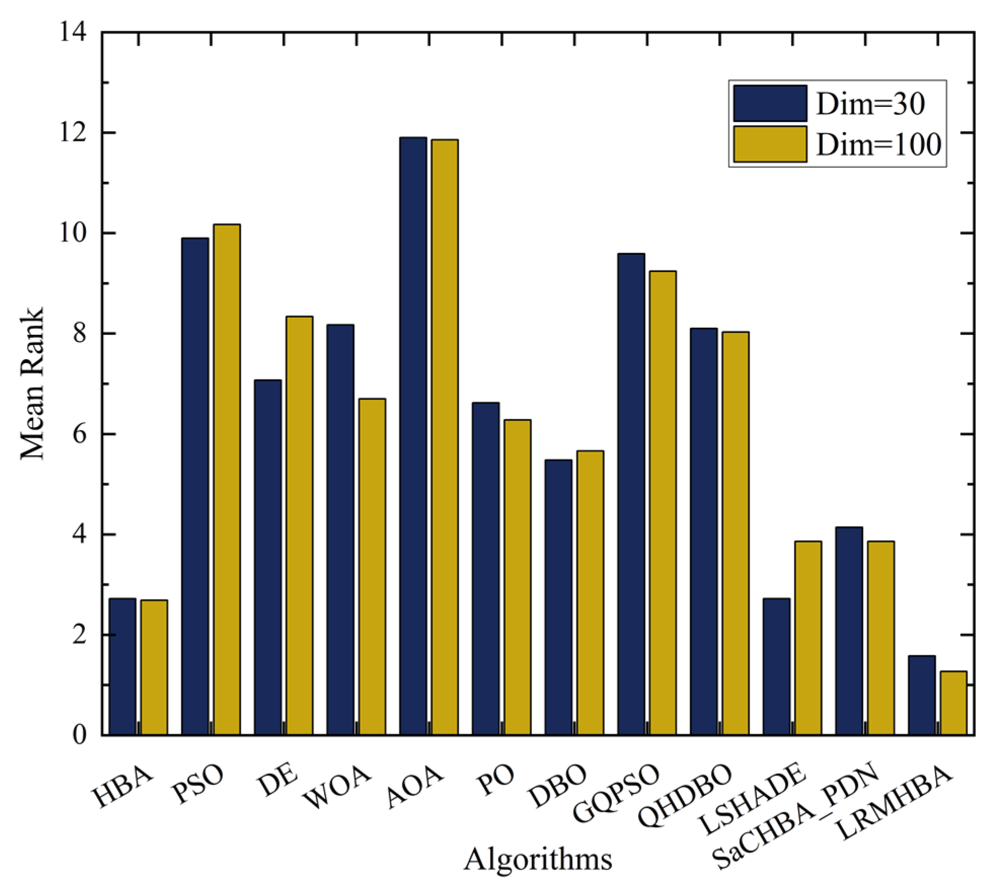
| Mean Rank | 2.72 | 9.90 | 7.07 | 8.17 | 11.90 | 6.62 | 5.48 | 9.59 | 8.10 | 2.72 | 4.14 | 1.58 | |
| Final Ranking | 2 | 11 | 7 | 9 | 12 | 6 | 5 | 10 | 8 | 2 | 4 | 1 | |
| Function | Index | HBA | PSO | DE | WOA | AOA | PO | DBO | GQPSO | QHDBO | LSHADE | SaCHBA_PDN | LRMHBA |
|---|---|---|---|---|---|---|---|---|---|---|---|---|---|
| CEC01 | Best | 1.822 × 10+7 | 2.767 × 10+11 | 1.773 × 10+11 | 2.415 × 10+9 | 5.206 × 10+11 | 2.056 × 10+10 | 3.831 × 10+9 | 1.623 × 10+11 | 7.078 × 10+09 | 5.225 × 10+3 | 2.535 × 10+7 | 1.166 × 10+5 |
| Mean | 1.558 × 10+9 | 3.326 × 10+11 | 2.199 × 10+11 | 3.875 × 10+9 | 6.059 × 10+11 | 3.809 × 10+10 | 1.673 × 10+10 | 1.657 × 10+11 | 3.036 × 10+10 | 2.716 × 10+9 | 3.066 × 10+8 | 1.247 × 10+6 | |
| Std | 1.853 × 10+9 | 3.193 × 10+10 | 1.241 × 10+10 | 1.026 × 10+9 | 3.294 × 10+10 | 9.365 × 10+9 | 2.158 × 10+10 | 1.802 × 10+9 | 1.202 × 10+10 | 8.337 × 10+9 | 5.054 × 10+8 | 1.138 × 10+6 | |
| Rank | 4 | 11 | 10 | 5 | 12 | 8 | 6 | 9 | 7 | 2 | 3 | 1 | |
| CEC03 | Best | 2.197 × 10+5 | 7.104 × 10+5 | 7.156 × 10+5 | 4.868 × 10+5 | 8.023 × 10+5 | 1.715 × 10+5 | 3.466 × 10+5 | 2.649 × 10+5 | 3.761 × 10+5 | 2.962 × 10+5 | 6.301 × 10+4 | 1.655 × 10+5 |
| Mean | 2.722 × 10+5 | 9.684 × 10+5 | 8.882 × 10+5 | 8.701 × 10+5 | 8.249 × 10+10 | 2.044 × 10+5 | 6.375 × 10+5 | 2.872 × 10+5 | 1.184 × 10+6 | 8.650 × 10+5 | 8.665 × 10+4 | 2.059 × 10+5 | |
| Std | 2.239 × 10+4 | 1.329 × 10+5 | 6.350 × 10+4 | 1.978 × 10+5 | 2.661 × 10+11 | 1.588 × 10+4 | 2.324 × 10+5 | 9.710 × 10+3 | 3.119 × 10+5 | 3.466 × 10+5 | 1.451 × 10+4 | 2.187 × 10+4 | |
| Rank | 4 | 10 | 8 | 7 | 12 | 2 | 6 | 5 | 11 | 9 | 1 | 3 | |
| CEC04 | Best | 7.874 × 10+2 | 3.907 × 10+4 | 3.310 × 10+4 | 1.534 × 10+03 | 1.894 × 10+5 | 2.208 × 10+3 | 1.281 × 10+3 | 3.136 × 10+4 | 2.113 × 10+3 | 4.976 × 10+2 | 7.942 × 10+2 | 7.001 × 10+2 |
| Mean | 9.253 × 10+2 | 6.342 × 10+4 | 3.802 × 10+4 | 2.410 × 10+03 | 2.693 × 10+5 | 3.864 × 10+3 | 3.021 × 10+3 | 3.438 × 10+4 | 6.928 × 10+3 | 2.372 × 10+3 | 9.884 × 10+2 | 7.725 × 10+2 | |
| Std | 9.496 × 10+1 | 1.704 × 10+4 | 2.411 × 10+3 | 5.914 × 10+02 | 3.821 × 10+4 | 8.715 × 10+2 | 2.804 × 10+3 | 1.233 × 10+3 | 4.368 × 10+3 | 8.155 × 10+3 | 1.547 × 10+2 | 4.891 × 10+1 | |
| Rank | 3 | 11 | 10 | 5 | 12 | 7 | 6 | 9 | 8 | 2 | 4 | 1 | |
| CEC05 | Best | 9.526 × 10+2 | 2.046 × 10+3 | 2.101 × 10+3 | 1.443 × 10+03 | 2.830 × 10+3 | 1.459 × 10+3 | 1.249 × 10+3 | 1.801 × 10+3 | 1.180 × 10+3 | 6.224 × 10+2 | 1.147 × 10+3 | 7.390 × 10+2 |
| Mean | 1.109 × 10+3 | 2.345 × 10+3 | 2.163 × 10+3 | 1.662 × 10+03 | 3.027 × 10+3 | 1.554 × 10+3 | 1.666 × 10+3 | 1.835 × 10+3 | 1.328 × 10+3 | 1.243 × 10+3 | 1.288 × 10+3 | 8.854 × 10+2 | |
| Std | 8.968 × 10+1 | 1.271 × 10+2 | 3.802 × 10+1 | 1.815 × 10+02 | 1.081 × 10+2 | 6.241 × 10+1 | 1.425 × 10+2 | 1.675 × 10+1 | 6.349 × 10+1 | 3.053 × 10+2 | 7.608 × 10+1 | 6.979 × 10+1 | |
| Rank | 2 | 11 | 10 | 7 | 12 | 6 | 8 | 9 | 5 | 3 | 4 | 1 | |
| CEC06 | Best | 6.258 × 10+2 | 7.132 × 10+2 | 6.775 × 10+2 | 6.784 × 10+02 | 7.473 × 10+2 | 6.719 × 10+2 | 6.477 × 10+2 | 6.856 × 10+2 | 6.481 × 10+2 | 6.000 × 10+2 | 6.549 × 10+2 | 6.010 × 10+2 |
| Mean | 6.375 × 10+2 | 7.247 × 10+2 | 6.858 × 10+2 | 6.927 × 10+02 | 7.609 × 10+2 | 6.812 × 10+2 | 6.727 × 10+2 | 6.906 × 10+2 | 6.546 × 10+2 | 6.149 × 10+2 | 6.634 × 10+2 | 6.031 × 10+2 | |
| Std | 7.000 × 10+0 | 6.883 × 10+0 | 3.096 × 10+0 | 9.670 × 10+00 | 6.521 × 10+0 | 5.067 × 10+0 | 9.215 × 10+0 | 2.162 × 10+0 | 4.094 × 10+0 | 2.964 × 10+1 | 4.470 × 10+0 | 1.402 × 10+0 | |
| Rank | 3 | 11 | 8 | 9 | 12 | 7 | 6 | 10 | 4 | 2 | 5 | 1 | |
| CEC07 | Best | 1.637 × 10+3 | 6.805 × 10+3 | 8.288 × 10+3 | 3.130 × 10+3 | 1.200 × 10+4 | 2.964 × 10+3 | 1.844 × 10+3 | 3.093 × 10+3 | 1.728 × 10+3 | 1.134 × 10+3 | 2.311 × 10+3 | 1.063 × 10+3 |
| Mean | 2.041 × 10+3 | 8.369 × 10+3 | 9.110 × 10+3 | 3.419 × 10+3 | 1.315 × 10+4 | 3.403 × 10+3 | 2.499 × 10+3 | 3.154 × 10+3 | 2.279 × 10+3 | 1.693 × 10+3 | 2.698 × 10+3 | 1.168 × 10+3 | |
| Std | 1.869 × 10+2 | 4.707 × 10+2 | 3.408 × 10+2 | 1.562 × 10+2 | 5.127 × 10+2 | 1.653 × 10+2 | 5.879 × 10+2 | 4.717 × 10+1 | 2.671 × 10+2 | 6.036 × 10+2 | 1.724 × 10+2 | 7.186 × 10+1 | |
| Rank | 3 | 10 | 11 | 9 | 12 | 8 | 5 | 7 | 4 | 2 | 6 | 1 | |
| CEC08 | Best | 1.206 × 10+3 | 2.388 × 10+3 | 2.365 × 10+3 | 1.858 × 10+3 | 3.098 × 10+3 | 1.850 × 10+3 | 1.658 × 10+3 | 2.154 × 10+3 | 1.499 × 10+3 | 1.008 × 10+3 | 1.480 × 10+3 | 1.045 × 10+3 |
| Mean | 1.387 × 10+3 | 2.645 × 10+3 | 2.452 × 10+3 | 2.106 × 10+3 | 3.464 × 10+3 | 1.989 × 10+3 | 1.989 × 10+3 | 2.199 × 10+3 | 1.669 × 10+3 | 1.616 × 10+3 | 1.618 × 10+3 | 1.126 × 10+3 | |
| Std | 7.768 × 10+1 | 1.426 × 10+2 | 4.199 × 10+1 | 1.519 × 10+2 | 1.399 × 10+2 | 8.957 × 10+1 | 1.540 × 10+2 | 1.801 × 10+1 | 9.639 × 10+1 | 3.752 × 10+2 | 8.558 × 10+1 | 5.226 × 10+1 | |
| Rank | 2 | 11 | 10 | 8 | 12 | 6 | 7 | 9 | 5 | 3 | 4 | 1 | |
| CEC09 | Best | 1.408 × 10+4 | 1.047 × 10+5 | 1.084 × 10+5 | 3.627 × 10+4 | 1.723 × 10+5 | 3.235 × 10+4 | 2.093 × 10+4 | 5.267 × 10+4 | 1.975 × 10+4 | 9.125 × 10+2 | 2.039 × 10+4 | 3.051 × 10+3 |
| Mean | 2.272 × 10+4 | 1.328 × 10+5 | 1.343 × 10+5 | 5.837 × 10+4 | 2.185 × 10+5 | 4.047 × 10+4 | 4.903 × 10+4 | 5.619 × 10+4 | 4.337 × 10+4 | 2.369 × 10+4 | 2.637 × 10+4 | 8.251 × 10+3 | |
| Std | 3.392 × 10+3 | 1.316 × 10+4 | 9.405 × 10+3 | 1.641 × 10+4 | 1.638 × 10+4 | 4.906 × 10+3 | 1.926 × 10+4 | 2.227 × 10+3 | 2.442 × 10+4 | 3.010 × 10+4 | 3.725 × 10+3 | 3.267 × 10+3 | |
| Rank | 2 | 10 | 11 | 8 | 12 | 6 | 7 | 9 | 5 | 3 | 4 | 1 | |
| CEC10 | Best | 1.280 × 10+4 | 3.161 × 10+4 | 2.841 × 10+4 | 2.081 × 10+4 | 3.419 × 10+4 | 1.825 × 10+4 | 1.268 × 10+4 | 2.876 × 10+4 | 3.846 × 10+4 | 1.841 × 10+4 | 1.597 × 10+4 | 1.232 × 10+4 |
| Mean | 1.712 × 10+4 | 3.243 × 10+4 | 2.931 × 10+4 | 2.585 × 10+4 | 3.600 × 10+4 | 2.295 × 10+4 | 1.794 × 10+4 | 3.010 × 10+4 | 3.846 × 10+4 | 2.795 × 10+4 | 2.135 × 10+4 | 1.615 × 10+4 | |
| Std | 3.252 × 10+3 | 4.542 × 10+2 | 3.760 × 10+2 | 2.660 × 10+3 | 7.878 × 10+2 | 2.206 × 10+3 | 1.671 × 10+3 | 4.993 × 10+2 | 2.220 × 10⁻¹¹ | 5.288 × 10+3 | 3.299 × 10+3 | 2.590 × 10+3 | |
| Rank | 2 | 10 | 8 | 6 | 11 | 5 | 3 | 9 | 12 | 7 | 4 | 1 | |
| CEC11 | Best | 4.326 × 10+3 | 1.619 × 10+5 | 1.309 × 10+5 | 3.089 × 10+4 | 4.148 × 10+5 | 1.446 × 10+4 | 2.884 × 10+4 | 8.732 × 10+4 | 7.063 × 10+4 | 7.525 × 10+3 | 2.882 × 10+3 | 3.058 × 10+3 |
| Mean | 6.248 × 10+3 | 2.469 × 10+5 | 1.795 × 10+5 | 8.670 × 10+4 | 2.633 × 10+7 | 2.475 × 10+4 | 9.970 × 10+4 | 9.384 × 10+4 | 2.097 × 10+5 | 1.087 × 10+5 | 4.575 × 10+3 | 4.352 × 10+3 | |
| Std | 1.986 × 10+3 | 6.108 × 10+4 | 2.083 × 10+4 | 5.175 × 10+4 | 7.664 × 10+7 | 6.078 × 10+3 | 3.971 × 10+4 | 3.974 × 10+3 | 1.019 × 10+5 | 8.240 × 10+4 | 1.101 × 10+3 | 1.314 × 10+3 | |
| Rank | 3 | 11 | 10 | 5 | 12 | 4 | 8 | 6 | 9 | 7 | 2 | 1 | |
| CEC12 | Best | 1.006 × 10+7 | 5.639 × 10+10 | 3.400 × 10+10 | 6.826 × 10+8 | 2.606 × 10+11 | 1.145 × 10+9 | 4.683 × 10+8 | 8.315 × 10+10 | 2.958 × 10+9 | 4.379 × 10+7 | 2.034 × 10+7 | 5.574 × 10+6 |
| Mean | 3.478 × 10+7 | 8.357 × 10+10 | 4.208 × 10+10 | 3.074 × 10+9 | 3.382 × 10+11 | 3.716 × 10+9 | 1.473 × 10+9 | 9.473 × 10+10 | 1.659 × 10+10 | 5.508 × 10+9 | 9.615 × 10+7 | 1.394 × 10+7 | |
| Std | 1.678 × 10+7 | 1.551 × 10+10 | 3.761 × 10+9 | 1.817 × 10+9 | 3.713 × 10+10 | 1.338 × 10+9 | 7.689 × 10+8 | 4.349 × 10+9 | 1.012 × 10+10 | 1.772 × 10+10 | 1.032 × 10+8 | 6.024 × 10+6 | |
| Rank | 2 | 10 | 9 | 6 | 12 | 7 | 5 | 11 | 8 | 4 | 3 | 1 | |
| CEC13 | Best | 1.513 × 10+4 | 7.198 × 10+9 | 1.036 × 10+9 | 2.575 × 10+6 | 7.090 × 10+10 | 4.193 × 10+6 | 1.568 × 10+5 | 1.615 × 10+10 | 6.455 × 10+6 | 1.868 × 10+3 | 4.061 × 10+4 | 2.857 × 10+3 |
| Mean | 2.957 × 10+4 | 1.380 × 10+10 | 1.462 × 10+9 | 7.742 × 10+6 | 8.886 × 10+10 | 1.659 × 10+8 | 7.644 × 10+7 | 1.885 × 10+10 | 3.121 × 10+9 | 6.916 × 10+6 | 1.320 × 10+5 | 8.822 × 10+3 | |
| Std | 9.707 × 10+3 | 3.383 × 10+9 | 1.698 × 10+8 | 6.456 × 10+6 | 9.725 × 10+9 | 2.077 × 10+8 | 9.377 × 10+7 | 1.352 × 10+9 | 3.420 × 10+9 | 3.370 × 10+7 | 1.112 × 10+5 | 6.487 × 10+3 | |
| Rank | 2 | 10 | 8 | 5 | 12 | 7 | 6 | 11 | 9 | 3 | 4 | 1 | |
| CEC14 | Best | 6.923 × 10+4 | 1.579 × 10+7 | 1.954 × 10+7 | 1.320 × 10+6 | 1.796 × 10+8 | 1.706 × 10+6 | 2.248 × 10+6 | 1.015 × 10+7 | 2.695 × 10+6 | 8.126 × 10+4 | 7.349 × 10+4 | 7.685 × 10+4 |
| Mean | 5.361 × 10+5 | 5.457 × 10+7 | 4.019 × 10+7 | 7.028 × 10+6 | 6.765 × 10+8 | 4.499 × 10+6 | 7.934 × 10+6 | 1.592 × 10+7 | 1.274 × 10+7 | 1.030 × 10+7 | 2.054 × 10+5 | 3.550 × 10+5 | |
| Std | 2.368 × 10+5 | 2.300 × 10+7 | 1.035 × 10+7 | 5.017 × 10+6 | 2.714 × 10+8 | 1.817 × 10+6 | 5.020 × 10+6 | 2.269 × 10+6 | 8.366 × 10+6 | 8.426 × 10+6 | 1.406 × 10+5 | 1.801 × 10+5 | |
| Rank | 3 | 11 | 10 | 5 | 12 | 4 | 6 | 9 | 8 | 7 | 1 | 2 | |
| CEC15 | Best | 3.560 × 10+3 | 2.437 × 10+9 | 1.078 × 10+8 | 2.397 × 10+5 | 3.599 × 10+10 | 7.263 × 10+4 | 4.477 × 10+4 | 5.942 × 10+9 | 5.583 × 10+4 | 1.809 × 10+3 | 1.640 × 10+4 | 1.904 × 10+3 |
| Mean | 1.015 × 10+4 | 5.356 × 10+9 | 1.854 × 10+8 | 9.925 × 10+5 | 4.253 × 10+10 | 1.500 × 10+7 | 8.312 × 10+6 | 7.069 × 10+9 | 2.065 × 10+9 | 1.549 × 10+7 | 9.354 × 10+4 | 4.952 × 10+3 | |
| Std | 7.725 × 10+3 | 1.723 × 10+9 | 4.443 × 10+7 | 7.510 × 10+5 | 5.405 × 10+09 | 2.088 × 10+7 | 2.723 × 10+7 | 5.516 × 10+8 | 2.679 × 10+9 | 5.771 × 10+7 | 1.261 × 10+5 | 5.687 × 10+3 | |
| Rank | 2 | 10 | 8 | 6 | 12 | 7 | 5 | 11 | 9 | 3 | 4 | 1 | |
| CEC16 | Best | 4.498 × 10+3 | 1.184 × 10+4 | 1.090 × 10+4 | 1.076 × 10+4 | 2.570 × 10+4 | 7.612 × 10+3 | 6.624 × 10+3 | 1.302 × 10+4 | 7.366 × 10+3 | 7.077 × 10+3 | 5.275 × 10+3 | 4.121 × 10+3 |
| Mean | 5.761 × 10+3 | 1.330 × 10+4 | 1.183 × 10+4 | 1.397 × 10+4 | 3.656 × 10+4 | 1.034 × 10+4 | 8.173 × 10+3 | 1.401 × 10+4 | 9.376 × 10+3 | 9.750 × 10+3 | 7.314 × 10+3 | 5.522 × 10+3 | |
| Std | 5.936 × 10+2 | 8.210 × 10+2 | 4.327 × 10+2 | 1.728 × 10+3 | 5.237 × 10+3 | 1.126 × 10+3 | 1.027 × 10+3 | 3.683 × 10+2 | 1.294 × 10+3 | 1.144 × 10+3 | 1.519 × 10+3 | 7.987 × 10+2 | |
| Rank | 2 | 9 | 8 | 10 | 12 | 7 | 4 | 11 | 5 | 6 | 3 | 1 | |
| CEC17 | Best | 3.919 × 10+3 | 1.312 × 10+4 | 8.541 × 10+3 | 6.004 × 10+3 | 1.210 × 10+7 | 5.488 × 10+3 | 5.643 × 10+3 | 1.494 × 10+4 | 6.877 × 10+3 | 6.041 × 10+3 | 5.280 × 10+3 | 3.459 × 10+3 |
| Mean | 5.021 × 10+3 | 5.133 × 10+4 | 9.477 × 10+3 | 7.875 × 10+3 | 6.376 × 10+7 | 7.579 × 10+3 | 7.900 × 10+3 | 2.767 × 10+4 | 9.458 × 10+4 | 8.250 × 10+3 | 6.410 × 10+3 | 4.822 × 10+3 | |
| Std | 5.535 × 10+2 | 8.347 × 10+4 | 4.699 × 10+2 | 9.812 × 10+2 | 3.607 × 10+7 | 1.691 × 10+3 | 9.708 × 10+2 | 5.655 × 10+3 | 4.140 × 10+5 | 3.391 × 10+3 | 6.239 × 10+2 | 6.304 × 10+2 | |
| Rank | 2 | 10 | 9 | 6 | 12 | 4 | 7 | 11 | 8 | 5 | 3 | 1 | |
| CEC18 | Best | 3.734 × 10+5 | 4.288 × 10+7 | 3.362 × 10+7 | 1.219 × 10+6 | 5.789 × 10+8 | 1.780 × 10+6 | 3.247 × 10+6 | 1.311 × 10+7 | 5.792 × 10+6 | 9.811 × 10+5 | 2.679 × 10+5 | 4.071 × 10+5 |
| Mean | 1.168 × 10+6 | 9.027 × 10+7 | 5.991 × 10+7 | 7.124 × 10+6 | 1.322 × 10+9 | 3.909 × 10+6 | 1.124 × 10+7 | 2.250 × 10+7 | 3.641 × 10+7 | 2.350 × 10+7 | 5.194 × 10+5 | 8.226 × 10+5 | |
| Std | 5.423 × 10+5 | 3.369 × 10+7 | 1.412 × 10+7 | 4.328 × 10+6 | 4.436 × 10+8 | 1.356 × 10+6 | 7.402 × 10+6 | 3.874 × 10+6 | 2.992 × 10+7 | 4.006 × 10+7 | 1.937 × 10+5 | 3.368 × 10+5 | |
| Rank | 3 | 11 | 10 | 5 | 12 | 4 | 6 | 8 | 9 | 7 | 1 | 2 | |
| CEC19 | Best | 2.362 × 10+3 | 1.525 × 10+9 | 1.706 × 10+8 | 3.862 × 10+6 | 2.891 × 10+10 | 7.189 × 10+6 | 5.677 × 10+4 | 4.994 × 10+9 | 3.456 × 10+6 | 2.020 × 10+3 | 2.718 × 10+4 | 2.097 × 10+3 |
| Mean | 9.591 × 10+3 | 4.438 × 10+9 | 3.217 × 10+8 | 3.166 × 10+7 | 4.353 × 10+10 | 5.270 × 10+7 | 2.407 × 10+7 | 6.136 × 10+9 | 6.314 × 10+8 | 6.601 × 10+5 | 1.385 × 10+5 | 5.417 × 10+3 | |
| Std | 9.660 × 10+3 | 1.617 × 10+9 | 6.736 × 10+7 | 2.212 × 10+7 | 6.647 × 10+9 | 1.164 × 10+8 | 2.388 × 10+7 | 5.959 × 10+8 | 1.027 × 10+9 | 1.812 × 10+6 | 1.410 × 10+5 | 4.125 × 10+3 | |
| Rank | 2 | 10 | 9 | 6 | 12 | 7 | 5 | 11 | 8 | 3 | 4 | 1 | |
| CEC20 | Best | 4.117 × 10+3 | 7.100 × 10+3 | 5.899 × 10+3 | 5.499 × 10+3 | 8.324 × 10+3 | 5.067 × 10+3 | 4.992 × 10+3 | 6.363 × 10+3 | 7.052 × 10+3 | 5.639 × 10+3 | 4.752 × 10+3 | 3.947 × 10+3 |
| Mean | 5.187 × 10+3 | 7.888 × 10+3 | 6.786 × 10+3 | 6.691 × 10+3 | 9.660 × 10+3 | 6.076 × 10+3 | 6.062 × 10+3 | 6.785 × 10+3 | 8.275 × 10+3 | 6.631 × 10+3 | 5.760 × 10+3 | 4.939 × 10+3 | |
| Std | 5.829 × 10+2 | 2.833 × 10+2 | 3.409 × 10+2 | 6.119 × 10+2 | 3.967 × 10+2 | 5.381 × 10+2 | 6.682 × 10+2 | 2.173 × 10+2 | 5.791 × 10+2 | 9.393 × 10+2 | 4.640 × 10+2 | 5.212 × 10+2 | |
| Rank | 2 | 10 | 9 | 7 | 12 | 4 | 5 | 8 | 11 | 6 | 3 | 1 | |
| CEC21 | Best | 2.695 × 10+3 | 4.050 × 10+3 | 3.874 × 10+3 | 3.765 × 10+3 | 5.034 × 10+3 | 3.390 × 10+3 | 3.371 × 10+3 | 3.803 × 10+3 | 3.555 × 10+3 | 2.638 × 10+3 | 3.166 × 10+3 | 2.510 × 10+3 |
| Mean | 2.843 × 10+3 | 4.281 × 10+3 | 4.022 × 10+3 | 4.314 × 10+3 | 5.345 × 10+3 | 3.690 × 10+3 | 3.572 × 10+3 | 3.860 × 10+3 | 4.177 × 10+3 | 3.081 × 10+3 | 3.392 × 10+3 | 2.606 × 10+3 | |
| Std | 8.851 × 10+1 | 1.453 × 10+2 | 5.202 × 10+1 | 2.531 × 10+2 | 1.687 × 10+2 | 1.736 × 10+2 | 1.121 × 10+2 | 3.111 × 10+1 | 3.462 × 10+2 | 3.466 × 10+2 | 1.350 × 10+2 | 8.632 × 10+1 | |
| Rank | 2 | 11 | 8 | 10 | 12 | 6 | 5 | 7 | 9 | 3 | 4 | 1 | |
| CEC22 | Best | 1.566 × 10+4 | 3.278 × 10+4 | 3.015 × 10+4 | 2.311 × 10+4 | 3.756 × 10+4 | 2.226 × 10+4 | 1.787 × 10+4 | 3.156 × 10+4 | 2.488 × 10+4 | 1.939 × 10+4 | 1.804 × 10+4 | 1.687 × 10+4 |
| Mean | 2.155 × 10+4 | 3.425 × 10+4 | 3.116 × 10+4 | 2.974 × 10+4 | 3.879 × 10+4 | 2.577 × 10+4 | 2.089 × 10+4 | 3.267 × 10+4 | 2.816 × 10+4 | 2.894 × 10+4 | 2.404 × 10+4 | 1.973 × 10+4 | |
| Std | 3.087 × 10+3 | 6.017 × 10+2 | 4.286 × 10+2 | 3.140 × 10+3 | 5.745 × 10+2 | 1.833 × 10+3 | 1.862 × 10+3 | 4.966 × 10+2 | 1.942 × 10+3 | 4.764 × 10+3 | 2.718 × 10+3 | 2.085 × 10+3 | |
| Rank | 3 | 11 | 9 | 8 | 12 | 5 | 2 | 10 | 6 | 7 | 4 | 1 | |
| CEC23 | Best | 3.258 × 10+3 | 4.605 × 10+3 | 3.927 × 10+3 | 4.754 × 10+3 | 7.376 × 10+3 | 4.276 × 10+3 | 3.892 × 10+3 | 5.625 × 10+3 | 8.724 × 10+3 | 3.019 × 10+3 | 3.833 × 10+3 | 3.016 × 10+3 |
| Mean | 3.441 × 10+3 | 5.011 × 10+3 | 3.993 × 10+3 | 5.337 × 10+3 | 8.159 × 10+3 | 4.568 × 10+3 | 4.219 × 10+3 | 5.792 × 10+3 | 8.724 × 10+3 | 3.494 × 10+3 | 4.468 × 10+3 | 3.161 × 10+3 | |
| Std | 1.064 × 10+2 | 2.425 × 10+2 | 2.209 × 10+1 | 3.041 × 10+2 | 4.690 × 10+2 | 1.744 × 10+2 | 1.514 × 10+2 | 7.152 × 10+1 | 3.700 × 10⁻¹² | 5.017 × 10+2 | 3.579 × 10+2 | 6.781 × 10+1 | |
| Rank | 3 | 8 | 4 | 9 | 11 | 7 | 5 | 10 | 12 | 2 | 6 | 1 | |
| CEC24 | Best | 3.664 × 10+3 | 5.194 × 10+3 | 4.461 × 10+3 | 5.694 × 10+3 | 1.160 × 10+4 | 4.938 × 10+3 | 4.526 × 10+3 | 7.587 × 10+3 | 1.423 × 10+4 | 3.461 × 10+3 | 4.580 × 10+3 | 3.539 × 10+3 |
| Mean | 4.124 × 10+3 | 5.979 × 10+3 | 4.588 × 10+3 | 6.951 × 10+3 | 1.376 × 10+4 | 5.811 × 10+3 | 5.027 × 10+3 | 7.950 × 10+3 | 1.423 × 10+4 | 4.054 × 10+3 | 5.707 × 10+3 | 3.637 × 10+3 | |
| Std | 4.932 × 10+2 | 4.214 × 10+2 | 3.501 × 10+1 | 6.592 × 10+2 | 9.340 × 10+2 | 3.934 × 10+2 | 2.571 × 10+2 | 1.489 × 10+2 | 7.400 × 10⁻¹² | 4.475 × 10+2 | 7.148 × 10+2 | 5.968 × 10+1 | |
| Rank | 3 | 8 | 4 | 9 | 11 | 7 | 5 | 10 | 12 | 2 | 6 | 1 | |
| CEC25 | Best | 3.409 × 10+3 | 3.893 × 10+4 | 4.672 × 10+4 | 4.294 × 10+3 | 8.876 × 10+4 | 5.121 × 10+3 | 3.540 × 10+3 | 1.421 × 10+4 | 3.589 × 10+3 | 3.270 × 10+3 | 3.478 × 10+3 | 3.251 × 10+3 |
| Mean | 3.612 × 10+3 | 5.584 × 10+4 | 5.561 × 10+4 | 4.678 × 10+3 | 1.256 × 10+5 | 5.888 × 10+3 | 8.259 × 10+3 | 1.489 × 10+4 | 4.368 × 10+3 | 6.534 × 10+3 | 3.630 × 10+3 | 3.449 × 10+3 | |
| Std | 8.397 × 10+1 | 7.960 × 10+3 | 4.866 × 10+3 | 3.824 × 10+2 | 1.773 × 10+4 | 4.766 × 10+2 | 4.612 × 10+3 | 2.262 × 10+2 | 5.622 × 10+2 | 1.073 × 10+4 | 9.013 × 10+1 | 6.705 × 10+1 | |
| Rank | 2 | 11 | 10 | 6 | 12 | 8 | 7 | 9 | 5 | 3 | 4 | 1 | |
| CEC26 | Best | 1.078 × 10+4 | 2.577 × 10+4 | 1.954 × 10+4 | 2.784 × 10+4 | 7.036 × 10+4 | 2.575 × 10+4 | 2.006 × 10+4 | 3.117 × 10+4 | 8.882 × 10+4 | 8.331 × 10+3 | 1.659 × 10+4 | 3.647 × 10+3 |
| Mean | 1.293 × 10+4 | 3.006 × 10+4 | 2.025 × 10+4 | 3.515 × 10+4 | 8.711 × 10+4 | 3.106 × 10+4 | 2.399 × 10+4 | 3.191 × 10+4 | 8.882 × 10+4 | 1.402 × 10+4 | 2.171 × 10+4 | 9.067 × 10+3 | |
| Std | 1.750 × 10+3 | 2.251 × 10+3 | 3.653 × 10+2 | 3.922 × 10+3 | 8.875 × 10+3 | 2.892 × 10+3 | 2.365 × 10+3 | 4.159 × 10+2 | 0.000 × 10+0 | 6.779 × 10+3 | 3.224 × 10+3 | 1.843 × 10+3 | |
| Rank | 2 | 7 | 4 | 10 | 11 | 8 | 6 | 9 | 12 | 3 | 5 | 1 | |
| CEC27 | Best | 3.561 × 10+3 | 4.416 × 10+3 | 3.980 × 10+3 | 3.200 × 10+3 | 1.427 × 10+4 | 4.042 × 10+3 | 3.579 × 10+3 | 7.453 × 10+3 | 3.840 × 10+3 | 3.200 × 10+3 | 3.760 × 10+3 | 3.439 × 10+3 |
| Mean | 4.087 × 10+3 | 5.181 × 10+3 | 4.188 × 10+3 | 3.200 × 10+3 | 1.667 × 10+4 | 4.596 × 10+3 | 4.015 × 10+3 | 7.922 × 10+3 | 4.419 × 10+3 | 3.200 × 10+3 | 4.418 × 10+3 | 3.684 × 10+3 | |
| Std | 5.506 × 10+2 | 5.009 × 10+2 | 7.984 × 10+1 | 2.477 × 10⁻⁴ | 1.417 × 10+3 | 4.180 × 10+2 | 2.380 × 10+2 | 2.039 × 10+2 | 3.514 × 10+2 | 4.285 × 10⁻⁴ | 4.331 × 10+2 | 2.093 × 10+2 | |
| Rank | 5 | 10 | 6 | 1 | 12 | 9 | 4 | 11 | 8 | 2 | 7 | 3 | |
| CEC28 | Best | 3.538 × 10+3 | 2.091 × 10+4 | 1.617 × 10+4 | 3.300 × 10+3 | 5.453 × 10+4 | 4.484 × 10+3 | 5.157 × 10+3 | 1.489 × 10+4 | 4.015 × 10+3 | 3.300 × 10+3 | 3.488 × 10+3 | 3.487 × 10+3 |
| Mean | 3.736 × 10+3 | 2.866 × 10+4 | 1.647 × 10+4 | 3.300 × 10+3 | 6.936 × 10+4 | 6.167 × 10+3 | 1.719 × 10+4 | 1.550 × 10+4 | 6.229 × 10+3 | 3.300 × 10+3 | 3.636 × 10+3 | 3.587 × 10+3 | |
| Std | 1.198 × 10+2 | 6.186 × 10+3 | 1.270 × 10+2 | 2.516 × 10⁻⁴ | 7.119 × 10+3 | 7.805 × 10+2 | 5.521 × 10+3 | 2.975 × 10+2 | 2.017 × 10+3 | 5.236 × 10⁻⁴ | 6.696 × 10+1 | 4.447 × 10+1 | |
| Rank | 5 | 11 | 9 | 2 | 12 | 7 | 10 | 8 | 6 | 1 | 4 | 3 | |
| CEC29 | Best | 5.485 × 10+3 | 1.727 × 10+4 | 1.116 × 10+4 | 7.946 × 10+3 | 2.209 × 10+6 | 1.022 × 10+4 | 8.291 × 10+3 | 2.341 × 10+4 | 7.287 × 10+3 | 5.980 × 10+3 | 7.787 × 10+3 | 5.005 × 10+3 |
| Mean | 6.779 × 10+3 | 3.155 × 10+4 | 1.229 × 10+4 | 1.448 × 10+4 | 1.418 × 10+7 | 1.393 × 10+4 | 1.013 × 10+4 | 2.894 × 10+4 | 1.970 × 10+4 | 9.354 × 10+3 | 1.089 × 10+4 | 6.361 × 10+3 | |
| Std | 6.611 × 10+2 | 8.819 × 10+3 | 5.543 × 10+2 | 2.800 × 10+3 | 9.130 × 10+6 | 1.752 × 10+3 | 9.695 × 10+2 | 3.487 × 10+3 | 1.561 × 10+4 | 2.806 × 10+3 | 1.386 × 10+3 | 5.860 × 10+2 | |
| Rank | 2 | 11 | 6 | 8 | 12 | 7 | 4 | 10 | 9 | 3 | 5 | 1 | |
| CEC30 | Best | 6.433 × 10+4 | 3.418 × 10+9 | 1.153 × 10+8 | 4.595 × 10+7 | 4.448 × 10+10 | 1.801 × 10+8 | 2.918 × 10+6 | 1.308 × 10+10 | 6.334 × 10+7 | 3.420 × 10+3 | 5.587 × 10+5 | 1.033 × 10+4 |
| Mean | 3.317 × 10+5 | 7.402 × 10+9 | 1.671 × 10+8 | 4.141 × 10+8 | 6.986 × 10+10 | 4.720 × 10+8 | 5.730 × 10+7 | 1.624 × 10+10 | 2.351 × 10+9 | 9.830 × 10+6 | 3.166 × 10+6 | 2.273 × 10+4 | |
| Std | 4.408 × 10+5 | 1.750 × 10+9 | 3.250 × 10+7 | 3.968 × 10+8 | 1.159 × 10+10 | 1.889 × 10+8 | 8.123 × 10+7 | 1.298 × 10+9 | 1.550 × 10+9 | 4.552 × 10+7 | 4.420 × 10+6 | 9.291 × 10+3 | |
| Rank | 3 | 10 | 6 | 7 | 12 | 8 | 5 | 11 | 9 | 2 | 4 | 1 | |
| Mean Rank | 2.69 | 10.17 | 8.34 | 6.7 | 11.86 | 6.28 | 5.66 | 9.24 | 8.03 | 3.86 | 3.86 | 1.27 | |
| Final Ranking | 2 | 11 | 9 | 7 | 12 | 6 | 5 | 10 | 8 | 3 | 3 | 1 | |
| Function | HBA | PSO | DE | WOA | AOA | PO | DBO | GQPSO | QHDBO | LSHADE | SaCHBA_PDN |
|---|---|---|---|---|---|---|---|---|---|---|---|
| CEC01 | 9.063 × 10⁻⁸ | 3.019 × 10⁻¹¹ | 3.019 × 10⁻¹¹ | 3.019 × 10⁻¹¹ | 3.019 × 10⁻¹¹ | 3.019 × 10⁻¹¹ | 3.019 × 10⁻¹¹ | 3.019 × 10⁻¹¹ | 3.019 × 10⁻¹¹ | 8.120 × 10⁻⁴ | 3.019 × 10⁻¹¹ |
| + | + | + | + | + | + | + | + | + | + | + | |
| CEC03 | 3.965 × 10⁻⁸ | 3.019 × 10⁻¹¹ | 3.019 × 10⁻¹¹ | 3.019 × 10⁻¹¹ | 3.019 × 10⁻¹¹ | 3.019 × 10⁻¹¹ | 3.019 × 10⁻¹¹ | 3.019 × 10⁻¹¹ | 3.019 × 10⁻¹¹ | 1.784 × 10⁻⁴ | 3.019 × 10⁻¹¹ |
| + | + | + | + | + | + | + | + | + | + | + | |
| CEC04 | 2.879 × 10⁻⁶ | 3.019 × 10⁻¹¹ | 3.019 × 10⁻¹¹ | 3.019 × 10⁻¹¹ | 3.019 × 10⁻¹¹ | 3.019 × 10⁻¹¹ | 3.019 × 10⁻¹¹ | 3.019 × 10⁻¹¹ | 3.019 × 10⁻¹¹ | 2.006 × 10⁻⁴ | 3.019 × 10⁻¹¹ |
| + | + | + | + | + | + | + | + | + | + | + | |
| CEC05 | 4.998 × 10⁻⁹ | 3.019 × 10⁻¹¹ | 3.019 × 10⁻¹¹ | 3.019 × 10⁻¹¹ | 3.019 × 10⁻¹¹ | 3.019 × 10⁻¹¹ | 3.019 × 10⁻¹¹ | 3.019 × 10⁻¹¹ | 3.019 × 10⁻¹¹ | 2.068 × 10⁻² | 3.019 × 10⁻¹¹ |
| + | + | + | + | + | + | + | + | + | + | + | |
| CEC06 | 4.998 × 10⁻⁹ | 3.019 × 10⁻¹¹ | 3.019 × 10⁻¹¹ | 3.019 × 10⁻¹¹ | 3.019 × 10⁻¹¹ | 3.019 × 10⁻¹¹ | 3.019 × 10⁻¹¹ | 3.019 × 10⁻¹¹ | 3.019 × 10⁻¹¹ | 3.006 × 10⁻⁴ | 3.019 × 10⁻¹¹ |
| + | + | + | + | + | + | + | + | + | + | + | |
| CEC07 | 5.186 × 10⁻⁷ | 3.019 × 10⁻¹¹ | 3.019 × 10⁻¹¹ | 3.019 × 10⁻¹¹ | 3.019 × 10⁻¹¹ | 3.019 × 10⁻¹¹ | 3.019 × 10⁻¹¹ | 3.019 × 10⁻¹¹ | 3.019 × 10⁻¹¹ | 1.114 × 10⁻³ | 3.019 × 10⁻¹¹ |
| + | + | + | + | + | + | + | + | + | + | + | |
| CEC08 | 1.492 × 10⁻⁶ | 3.019 × 10⁻¹¹ | 3.019 × 10⁻¹¹ | 3.019 × 10⁻¹¹ | 3.019 × 10⁻¹¹ | 3.019 × 10⁻¹¹ | 3.019 × 10⁻¹¹ | 3.019 × 10⁻¹¹ | 3.019 × 10⁻¹¹ | 8.197 × 10⁻⁷ | 3.019 × 10⁻¹¹ |
| + | + | + | + | + | + | + | + | + | + | + | |
| CEC09 | 3.094 × 10⁻⁶ | 3.019 × 10⁻¹¹ | 3.019 × 10⁻¹¹ | 3.019 × 10⁻¹¹ | 3.019 × 10⁻¹¹ | 3.019 × 10⁻¹¹ | 3.019 × 10⁻¹¹ | 3.019 × 10⁻¹¹ | 3.019 × 10⁻¹¹ | 4.982 × 10⁻⁴ | 3.019 × 10⁻¹¹ |
| + | + | + | + | + | + | + | + | + | + | + | |
| CEC10 | 5.462 × 10⁻⁹ | 3.019 × 10⁻¹¹ | 3.019 × 10⁻¹¹ | 3.019 × 10⁻¹¹ | 3.019 × 10⁻¹¹ | 3.019 × 10⁻¹¹ | 3.019 × 10⁻¹¹ | 3.019 × 10⁻¹¹ | 3.019 × 10⁻¹¹ | 5.874 × 10⁻⁴ | 3.019 × 10⁻¹¹ |
| + | + | + | + | + | + | + | + | + | + | + | |
| CEC11 | 4.801 × 10⁻⁷ | 3.019 × 10⁻¹¹ | 3.019 × 10⁻¹¹ | 3.019 × 10⁻¹¹ | 3.019 × 10⁻¹¹ | 3.019 × 10⁻¹¹ | 3.019 × 10⁻¹¹ | 3.019 × 10⁻¹¹ | 3.019 × 10⁻¹¹ | 4.856 × 10⁻³ | 3.019 × 10⁻¹¹ |
| + | + | + | + | + | + | + | + | + | + | + | |
| CEC12 | 3.646 × 10⁻⁸ | 3.019 × 10⁻¹¹ | 3.019 × 10⁻¹¹ | 3.019 × 10⁻¹¹ | 3.019 × 10⁻¹¹ | 3.019 × 10⁻¹¹ | 3.019 × 10⁻¹¹ | 3.019 × 10⁻¹¹ | 3.019 × 10⁻¹¹ | 3.835 × 10⁻⁶ | 3.019 × 10⁻¹¹ |
| + | + | + | + | + | + | + | + | + | + | + | |
| CEC13 | 6.518 × 10⁻⁹ | 3.019 × 10⁻¹¹ | 3.019 × 10⁻¹¹ | 3.019 × 10⁻¹¹ | 3.019 × 10⁻¹¹ | 3.019 × 10⁻¹¹ | 3.019 × 10⁻¹¹ | 3.019 × 10⁻¹¹ | 3.019 × 10⁻¹¹ | 3.006 × 10⁻⁴ | 3.019 × 10⁻¹¹ |
| + | + | + | + | + | + | + | + | + | + | + | |
| CEC14 | 7.043 × 10⁻⁷ | 3.019 × 10⁻¹¹ | 3.019 × 10⁻¹¹ | 3.019 × 10⁻¹¹ | 3.019 × 10⁻¹¹ | 3.019 × 10⁻¹¹ | 3.019 × 10⁻¹¹ | 3.019 × 10⁻¹¹ | 4.975 × 10⁻¹¹ | 2.531 × 10⁻⁴ | 3.019 × 10⁻¹¹ |
| + | + | + | + | + | + | + | + | + | + | + | |
| CEC15 | 5.600 × 10⁻⁷ | 3.019 × 10⁻¹¹ | 3.019 × 10⁻¹¹ | 3.019 × 10⁻¹¹ | 3.019 × 10⁻¹¹ | 3.019 × 10⁻¹¹ | 3.019 × 10⁻¹¹ | 3.019 × 10⁻¹¹ | 3.019 × 10⁻¹¹ | 2.709 × 10⁻² | 3.019 × 10⁻¹¹ |
| + | + | + | + | + | + | + | + | + | + | + | |
| CEC16 | 4.311 × 10⁻⁸ | 3.019 × 10⁻¹¹ | 3.019 × 10⁻¹¹ | 3.019 × 10⁻¹¹ | 3.019 × 10⁻¹¹ | 3.019 × 10⁻¹¹ | 3.019 × 10⁻¹¹ | 3.019 × 10⁻¹¹ | 3.019 × 10⁻¹¹ | 1.996 × 10⁻⁵ | 3.019 × 10⁻¹¹ |
| + | + | + | + | + | + | + | + | + | + | + | |
| CEC17 | 2.195 × 10⁻⁸ | 3.019 × 10⁻¹¹ | 3.019 × 10⁻¹¹ | 3.019 × 10⁻¹¹ | 3.019 × 10⁻¹¹ | 3.019 × 10⁻¹¹ | 3.019 × 10⁻¹¹ | 3.019 × 10⁻¹¹ | 3.019 × 10⁻¹¹ | 4.060 × 10⁻² | 3.019 × 10⁻¹¹ |
| + | + | + | + | + | + | + | + | + | + | + | |
| CEC18 | 1.102 × 10⁻⁸ | 3.019 × 10⁻¹¹ | 3.019 × 10⁻¹¹ | 3.019 × 10⁻¹¹ | 3.019 × 10⁻¹¹ | 3.019 × 10⁻¹¹ | 3.019 × 10⁻¹¹ | 3.019 × 10⁻¹¹ | 3.019 × 10⁻¹¹ | 8.564 × 10⁻⁴ | 3.019 × 10⁻¹¹ |
| + | + | + | + | + | + | + | + | + | + | + | |
| CEC19 | 1.850 × 10⁻⁸ | 3.019 × 10⁻¹¹ | 3.019 × 10⁻¹¹ | 3.019 × 10⁻¹¹ | 3.019 × 10⁻¹¹ | 3.019 × 10⁻¹¹ | 3.019 × 10⁻¹¹ | 3.019 × 10⁻¹¹ | 3.019 × 10⁻¹¹ | 2.278 × 10⁻⁵ | 3.019 × 10⁻¹¹ |
| + | + | + | + | + | + | + | + | + | + | + | |
| CEC20 | 4.444 × 10⁻⁷ | 3.019 × 10⁻¹¹ | 3.019 × 10⁻¹¹ | 3.019 × 10⁻¹¹ | 3.019 × 10⁻¹¹ | 3.019 × 10⁻¹¹ | 3.019 × 10⁻¹¹ | 3.019 × 10⁻¹¹ | 3.019 × 10⁻¹¹ | 2.891 × 10⁻³ | 3.019 × 10⁻¹¹ |
| + | + | + | + | + | + | + | + | + | + | + | |
| CEC21 | 9.063 × 10⁻⁸ | 3.019 × 10⁻¹¹ | 3.019 × 10⁻¹¹ | 3.019 × 10⁻¹¹ | 3.019 × 10⁻¹¹ | 3.019 × 10⁻¹¹ | 3.019 × 10⁻¹¹ | 3.019 × 10⁻¹¹ | 3.019 × 10⁻¹¹ | 6.913 × 10⁻⁴ | 3.019 × 10⁻¹¹ |
| + | + | + | + | + | + | + | + | + | + | + | |
| CEC22 | 5.092 × 10⁻⁸ | 3.019 × 10⁻¹¹ | 3.019 × 10⁻¹¹ | 3.019 × 10⁻¹¹ | 3.019 × 10⁻¹¹ | 3.019 × 10⁻¹¹ | 3.019 × 10⁻¹¹ | 3.019 × 10⁻¹¹ | 1.777 × 10⁻¹⁰ | 8.292 × 10⁻⁶ | 3.019 × 10⁻¹¹ |
| + | + | + | + | + | + | + | + | + | + | + | |
| CEC23 | 3.646 × 10−08 | 3.019 × 10⁻¹¹ | 3.019 × 10⁻¹¹ | 3.019 × 10⁻¹¹ | 3.019 × 10⁻¹¹ | 3.019 × 10⁻¹¹ | 3.019 × 10⁻¹¹ | 3.019 × 10⁻¹¹ | 3.019 × 10⁻¹¹ | 1.058 × 10⁻³ | 3.019 × 10⁻¹¹ |
| + | + | + | + | + | + | + | + | + | + | + | |
| CEC24 | 3.081 × 10−08 | 3.019 × 10⁻¹¹ | 3.019 × 10⁻¹¹ | 3.019 × 10⁻¹¹ | 3.019 × 10⁻¹¹ | 3.019 × 10⁻¹¹ | 3.019 × 10⁻¹¹ | 3.019 × 10⁻¹¹ | 3.019 × 10⁻¹¹ | 8.771 × 10⁻² | 3.019 × 10⁻¹¹ |
| + | + | + | + | + | + | + | + | + | - | + | |
| CEC25 | 1.206 × 10⁻¹⁰ | 3.002 × 10⁻¹¹ | 3.019 × 10⁻¹¹ | 3.019 × 10⁻¹¹ | 3.019 × 10⁻¹¹ | 3.019 × 10⁻¹¹ | 3.019 × 10⁻¹¹ | 3.019 × 10⁻¹¹ | 3.019 × 10⁻¹¹ | 5.091 × 10⁻⁶ | 3.019 × 10⁻¹¹ |
| + | + | + | + | + | + | + | + | + | + | + | |
| CEC26 | 2.390 × 10−08 | 3.019 × 10⁻¹¹ | 3.019 × 10⁻¹¹ | 3.019 × 10⁻¹¹ | 3.019 × 10⁻¹¹ | 3.019 × 10⁻¹¹ | 3.019 × 10⁻¹¹ | 3.019 × 10⁻¹¹ | 3.019 × 10⁻¹¹ | 2.510 × 10⁻² | 3.019 × 10⁻¹¹ |
| + | + | + | + | + | + | + | + | + | + | + | |
| CEC27 | 3.646 × 10−08 | 3.019 × 10⁻¹¹ | 3.019 × 10⁻¹¹ | 3.019 × 10⁻¹¹ | 3.019 × 10⁻¹¹ | 3.019 × 10⁻¹¹ | 3.019 × 10⁻¹¹ | 3.019 × 10⁻¹¹ | 3.019 × 10⁻¹¹ | 5.943 × 10⁻² | 3.019 × 10⁻¹¹ |
| + | + | + | + | + | + | + | + | + | - | + | |
| CEC28 | 2.602 × 10−08 | 3.019 × 10⁻¹¹ | 3.019 × 10⁻¹¹ | 3.019 × 10⁻¹¹ | 3.019 × 10⁻¹¹ | 3.019 × 10⁻¹¹ | 3.019 × 10⁻¹¹ | 3.019 × 10⁻¹¹ | 3.019 × 10⁻¹¹ | 4.353 × 10⁻⁵ | 3.019 × 10⁻¹¹ |
| + | + | + | + | + | + | + | + | + | + | + | |
| CEC29 | 6.010 × 10−08 | 3.019 × 10⁻¹¹ | 3.019 × 10⁻¹¹ | 3.019 × 10⁻¹¹ | 3.019 × 10⁻¹¹ | 3.019 × 10⁻¹¹ | 3.019 × 10⁻¹¹ | 3.019 × 10⁻¹¹ | 3.019 × 10⁻¹¹ | 4.226 × 10⁻³ | 3.019 × 10⁻¹¹ |
| + | + | + | + | + | + | + | + | + | + | + | |
| CEC30 | 6.528 × 10−08 | 3.019 × 10⁻¹¹ | 3.019 × 10⁻¹¹ | 3.019 × 10⁻¹¹ | 3.019 × 10⁻¹¹ | 3.019 × 10⁻¹¹ | 3.019 × 10⁻¹¹ | 3.019 × 10⁻¹¹ | 3.019 × 10⁻¹¹ | 2.002 × 10⁻⁶ | 3.019 × 10⁻¹¹ |
| + | + | + | + | + | + | + | + | + | + | + | |
| +/=/- | 29/0/0 | 29/0/0 | 29/0/0 | 29/0/0 | 29/0/0 | 29/0/0 | 29/0/0 | 29/0/0 | 29/0/0 | 27/0/2 | 29/0/0 |
| Funciton | Index | HBA | LRMHBA1 | LRMHBA2 | LRMHBA3 | LRMHBA |
|---|---|---|---|---|---|---|
| CEC01 | Best | 1.012 × 10+2 | 1.013 × 10+2 | 1.025 × 10+2 | 1.190 × 10+2 | 1.150 × 10+2 |
| Mean | 6.561 × 10+3 | 5.258 × 10+3 | 3.687 × 10+3 | 5.393 × 10+3 | 3.302 × 10+3 | |
| Std | 7.134 × 10+3 | 5.978 × 10+3 | 3.596 × 10+3 | 4.856 × 10+3 | 3.827 × 10+3 | |
| Rank | 5 | 3 | 2 | 4 | 1 | |
| CEC03 | Best | 1.248 × 10+3 | 7.671 × 10+2 | 1.552 × 10+3 | 3.036 × 10+2 | 3.048 × 10+2 |
| Mean | 3.231 × 10+3 | 3.584 × 10+3 | 4.083 × 10+3 | 4.298 × 10+2 | 9.780 × 10+2 | |
| Std | 1.327 × 10+3 | 3.115 × 10+3 | 1.529 × 10+3 | 1.707 × 10+2 | 1.959 × 10+3 | |
| Rank | 4 | 3 | 5 | 1 | 2 | |
| CEC04 | Best | 4.049 × 10+2 | 4.138 × 10+2 | 4.601 × 10+2 | 4.010 × 10+2 | 4.001 × 10+2 |
| Mean | 4.818 × 10+2 | 4.804 × 10+2 | 4.912 × 10+2 | 4.855 × 10+2 | 4.824 × 10+2 | |
| Std | 2.386 × 10+1 | 2.517 × 10+1 | 1.758 × 10+1 | 2.070 × 10+1 | 2.875 × 10+1 | |
| Rank | 1 | 3 | 5 | 4 | 2 | |
| CEC05 | Best | 5.497 × 10+2 | 5.647 × 10+2 | 5.348 × 10+2 | 5.348 × 10+2 | 5.229 × 10+2 |
| Mean | 6.041 × 10+2 | 6.234 × 10+2 | 5.698 × 10+2 | 5.662 × 10+2 | 5.551 × 10+2 | |
| Std | 2.948 × 10+1 | 3.347 × 10+1 | 2.041 × 10+1 | 1.651 × 10+1 | 1.852 × 10+1 | |
| Rank | 4 | 5 | 3 | 2 | 1 | |
| CEC06 | Best | 6.004 × 10+2 | 6.006 × 10+2 | 6.001 × 10+2 | 6.000 × 10+2 | 6.000 × 10+2 |
| Mean | 6.043 × 10+2 | 6.065 × 10+2 | 6.003 × 10+2 | 6.000 × 10+2 | 6.080 × 10+2 | |
| Std | 4.665 × 10+0 | 5.925 × 10+0 | 2.303 × 10⁻¹ | 3.328 × 10⁻³ | 3.035 × 10+1 | |
| Rank | 4 | 5 | 3 | 2 | 1 | |
| CEC07 | Best | 7.944 × 10+2 | 7.905 × 10+2 | 7.622 × 10+2 | 7.641 × 10+2 | 7.575 × 10+2 |
| Mean | 8.575 × 10+2 | 8.722 × 10+2 | 7.957 × 10+2 | 8.021 × 10+2 | 7.810 × 10+2 | |
| Std | 3.717 × 10+1 | 4.464 × 10+1 | 1.798 × 10+1 | 2.602 × 10+1 | 1.454 × 10+1 | |
| Rank | 4 | 5 | 2 | 3 | 1 | |
| CEC08 | Best | 8.557 × 10+2 | 8.458 × 10+2 | 8.408 × 10+2 | 8.368 × 10+2 | 8.388 × 10+2 |
| Mean | 8.972 × 10+2 | 8.993 × 10+2 | 8.650 × 10+2 | 8.646 × 10+2 | 8.588 × 10+2 | |
| Std | 2.153 × 10+1 | 1.991 × 10+1 | 1.197 × 10+1 | 1.759 × 10+1 | 1.462 × 10+1 | |
| Rank | 4 | 5 | 3 | 2 | 1 | |
| CEC09 | Best | 1.070 × 10+3 | 1.033 × 10+3 | 9.039 × 10+2 | 9.003 × 10+2 | 9.000 × 10+2 |
| Mean | 2.049 × 10+3 | 2.426 × 10+3 | 9.460 × 10+2 | 9.943 × 10+2 | 9.043 × 10+2 | |
| Std | 6.578 × 10+2 | 8.011 × 10+2 | 4.096 × 10+1 | 2.297 × 10+2 | 7.905 × 10+0 | |
| Rank | 4 | 5 | 3 | 2 | 1 | |
| CEC10 | Best | 3.491 × 10+3 | 3.689 × 10+3 | 4.443 × 10+3 | 3.174 × 10+3 | 3.569 × 10+3 |
| Mean | 4.821 × 10+3 | 5.268 × 10+3 | 5.879 × 10+3 | 4.615 × 10+3 | 5.079 × 10+3 | |
| Std | 9.057 × 10+2 | 1.204 × 10+3 | 1.053 × 10+3 | 7.697 × 10+2 | 8.708 × 10+2 | |
| Rank | 2 | 4 | 5 | 1 | 3 | |
| CEC11 | Best | 1.145 × 10+3 | 1.130 × 10+3 | 1.114 × 10+3 | 1.119 × 10+3 | 1.114 × 10+3 |
| Mean | 1.226 × 10+3 | 1.215 × 10+3 | 1.178 × 10+3 | 1.147 × 10+3 | 1.139 × 10+3 | |
| Std | 4.197 × 10+1 | 4.861 × 10+1 | 4.143 × 10+1 | 2.734 × 10+1 | 2.272 × 10+1 | |
| Rank | 5 | 4 | 3 | 2 | 1 | |
| CEC12 | Best | 1.090 × 10+4 | 8.781 × 10+3 | 2.404 × 10+4 | 5.149 × 10+3 | 8.858 × 10+3 |
| Mean | 7.432 × 10+4 | 8.874 × 10+4 | 9.861 × 10+4 | 3.602 × 10+4 | 6.223 × 10+8 | |
| Std | 6.303 × 10+4 | 9.746 × 10+4 | 8.322 × 10+4 | 2.397 × 10+4 | 3.409 × 10+9 | |
| Rank | 4 | 3 | 5 | 1 | 2 | |
| CEC13 | Best | 5.638 × 10+3 | 2.675 × 10+3 | 1.678 × 10+3 | 1.467 × 10+3 | 1.343 × 10+3 |
| Mean | 3.419 × 10+4 | 3.242 × 10+4 | 1.820 × 10+4 | 1.794 × 10+4 | 2.665 × 10+4 | |
| Std | 3.530 × 10+4 | 2.202 × 10+4 | 1.915 × 10+4 | 1.842 × 10+4 | 2.312 × 10+4 | |
| Rank | 4 | 5 | 2 | 1 | 3 | |
| CEC14 | Best | 1.977 × 10+3 | 1.925 × 10+3 | 1.834 × 10+3 | 1.695 × 10+3 | 1.548 × 10+3 |
| Mean | 9.720 × 10+3 | 8.360 × 10+3 | 1.374 × 10+4 | 3.874 × 10+3 | 3.695 × 10+3 | |
| Std | 1.157 × 10+4 | 6.583 × 10+3 | 1.068 × 10+4 | 2.741 × 10+3 | 2.118 × 10+3 | |
| Rank | 3 | 4 | 5 | 2 | 1 | |
| CEC15 | Best | 2.215 × 10+3 | 1.881 × 10+3 | 1.715 × 10+3 | 1.657 × 10+3 | 1.524 × 10+3 |
| Mean | 1.489 × 10+4 | 1.353 × 10+4 | 9.104 × 10+3 | 1.002 × 10+4 | 1.418 × 10+8 | |
| Std | 1.970 × 10+4 | 1.456 × 10+4 | 9.948 × 10+3 | 1.095 × 10+4 | 7.764 × 10+8 | |
| Rank | 5 | 4 | 3 | 2 | 1 | |
| CEC16 | Best | 1.910 × 10+3 | 1.977 × 10+3 | 1.883 × 10+3 | 1.871 × 10+3 | 1.746 × 10+3 |
| Mean | 2.607 × 10+3 | 2.619 × 10+3 | 2.449 × 10+3 | 2.620 × 10+3 | 2.882 × 10+3 | |
| Std | 2.702 × 10+2 | 3.939 × 10+2 | 2.850 × 10+2 | 3.874 × 10+2 | 2.691 × 10+3 | |
| Rank | 3 | 4 | 1 | 5 | 2 | |
| CEC17 | Best | 1.915 × 10+3 | 1.800 × 10+3 | 1.741 × 10+3 | 1.748 × 10+3 | 1.737 × 10+3 |
| Mean | 2.103 × 10+3 | 2.158 × 10+3 | 1.991 × 10+3 | 2.090 × 10+3 | 2.043 × 10+3 | |
| Std | 1.466 × 10+2 | 2.355 × 10+2 | 1.712 × 10+2 | 2.031 × 10+2 | 1.914 × 10+2 | |
| Rank | 4 | 5 | 1 | 3 | 2 | |
| CEC18 | Best | 2.251 × 10+4 | 3.658 × 10+4 | 4.196 × 10+4 | 7.205 × 10+3 | 1.199 × 10+4 |
| Mean | 1.818 × 10+5 | 2.476 × 10+5 | 2.789 × 10+5 | 8.728 × 10+4 | 8.309 × 10+4 | |
| Std | 1.752 × 10+5 | 2.327 × 10+5 | 2.479 × 10+5 | 7.751 × 10+4 | 5.484 × 10+4 | |
| Rank | 3 | 4 | 5 | 1 | 2 | |
| CEC19 | Best | 2.089 × 10+3 | 2.029 × 10+3 | 1.933 × 10+3 | 1.933 × 10+3 | 1.924 × 10+3 |
| Mean | 1.143 × 10+4 | 1.034 × 10+4 | 1.095 × 10+4 | 1.121 × 10+4 | 9.254 × 10+3 | |
| Std | 1.408 × 10+4 | 1.475 × 10+4 | 1.398 × 10+4 | 1.132 × 10+4 | 1.102 × 10+4 | |
| Rank | 4 | 2 | 1 | 5 | 3 | |
| CEC20 | Best | 2.125 × 10+3 | 2.205 × 10+3 | 2.140 × 10+3 | 2.057 × 10+3 | 2.045 × 10+3 |
| Mean | 2.464 × 10+3 | 2.503 × 10+3 | 2.491 × 10+3 | 2.406 × 10+3 | 2.479 × 10+3 | |
| Std | 2.135 × 10+2 | 1.729 × 10+2 | 2.067 × 10+2 | 2.249 × 10+2 | 2.277 × 10+2 | |
| Rank | 2 | 5 | 3 | 1 | 4 | |
| CEC21 | Best | 2.345 × 10+3 | 2.200 × 10+3 | 2.327 × 10+3 | 2.332 × 10+3 | 2.328 × 10+3 |
| Mean | 2.399 × 10+3 | 2.388 × 10+3 | 2.357 × 10+3 | 2.359 × 10+3 | 2.351 × 10+3 | |
| Std | 3.286 × 10+1 | 4.583 × 10+1 | 1.912 × 10+1 | 1.513 × 10+1 | 1.364 × 10+1 | |
| Rank | 5 | 4 | 2 | 3 | 1 | |
| CEC22 | Best | 2.300 × 10+3 | 2.300 × 10+3 | 2.300 × 10+3 | 2.300 × 10+3 | 2.300 × 10+3 |
| Mean | 3.404 × 10+3 | 3.662 × 10+3 | 3.992 × 10+3 | 3.616 × 10+3 | 4.077 × 10+3 | |
| Std | 2.057 × 10+3 | 2.193 × 10+3 | 2.482 × 10+3 | 2.093 × 10+3 | 2.276 × 10+3 | |
| Rank | 3 | 4 | 5 | 1 | 2 | |
| CEC23 | Best | 2.701 × 10+3 | 2.706 × 10+3 | 2.691 × 10+3 | 2.400 × 10+3 | 2.679 × 10+3 |
| Mean | 2.760 × 10+3 | 2.776 × 10+3 | 2.720 × 10+3 | 2.718 × 10+3 | 2.710 × 10+3 | |
| Std | 3.013 × 10+1 | 5.079 × 10+1 | 1.871 × 10+1 | 6.572 × 10+1 | 1.696 × 10+1 | |
| Rank | 4 | 5 | 2 | 3 | 1 | |
| CEC24 | Best | 2.893 × 10+3 | 2.870 × 10+3 | 2.848 × 10+3 | 2.853 × 10+3 | 2.859 × 10+3 |
| Mean | 2.960 × 10+3 | 3.009 × 10+3 | 2.875 × 10+3 | 2.923 × 10+3 | 2.884 × 10+3 | |
| Std | 8.248 × 10+1 | 1.994 × 10+2 | 1.511 × 10+1 | 9.380 × 10+1 | 1.750 × 10+1 | |
| Rank | 4 | 5 | 1 | 3 | 2 | |
| CEC25 | Best | 2.884 × 10+3 | 2.884 × 10+3 | 2.884 × 10+3 | 2.884 × 10+3 | 2.883 × 10+3 |
| Mean | 2.894 × 10+3 | 2.891 × 10+3 | 2.888 × 10+3 | 2.887 × 10+3 | 3.114 × 10+3 | |
| Std | 1.386 × 10+1 | 1.241 × 10+1 | 1.034 × 10+1 | 4.884 × 10+0 | 1.244 × 10+3 | |
| Rank | 5 | 4 | 1 | 2 | 3 | |
| CEC26 | Best | 2.800 × 10+3 | 2.800 × 10+3 | 2.900 × 10+3 | 2.900 × 10+3 | 2.900 × 10+3 |
| Mean | 4.662 × 10+3 | 4.275 × 10+3 | 4.200 × 10+3 | 4.450 × 10+3 | 4.174 × 10+3 | |
| Std | 6.194 × 10+2 | 9.792 × 10+2 | 3.730 × 10+2 | 4.136 × 10+2 | 2.791 × 10+2 | |
| Rank | 5 | 4 | 1 | 3 | 2 | |
| CEC27 | Best | 3.210 × 10+3 | 3.217 × 10+3 | 3.200 × 10+3 | 3.204 × 10+3 | 3.210 × 10+3 |
| Mean | 3.309 × 10+3 | 3.403 × 10+3 | 3.250 × 10+3 | 3.269 × 10+3 | 3.355 × 10+3 | |
| Std | 1.130 × 10+2 | 3.264 × 10+2 | 3.441 × 10+1 | 5.323 × 10+1 | 6.116 × 10+2 | |
| Rank | 4 | 5 | 2 | 3 | 1 | |
| CEC28 | Best | 3.100 × 10+3 | 3.162 × 10+3 | 3.123 × 10+3 | 3.102 × 10+3 | 3.142 × 10+3 |
| Mean | 3.367 × 10+3 | 3.224 × 10+3 | 3.316 × 10+3 | 3.200 × 10+3 | 3.215 × 10+3 | |
| Std | 8.128 × 10+2 | 3.479 × 10+1 | 5.677 × 10+2 | 3.901 × 10+1 | 3.406 × 10+1 | |
| Rank | 5 | 4 | 3 | 1 | 2 | |
| CEC29 | Best | 3.405 × 10+3 | 3.513 × 10+3 | 3.439 × 10+3 | 3.359 × 10+3 | 3.361 × 10+3 |
| Mean | 4.128 × 10+3 | 4.169 × 10+3 | 3.917 × 10+3 | 3.927 × 10+3 | 3.790 × 10+3 | |
| Std | 4.674 × 10+2 | 6.253 × 10+2 | 2.859 × 10+2 | 4.243 × 10+2 | 2.776 × 10+2 | |
| Rank | 5 | 4 | 2 | 3 | 1 | |
| CEC30 | Best | 6.976 × 10+3 | 6.156 × 10+3 | 5.882 × 10+3 | 5.577 × 10+3 | 5.074 × 10+3 |
| Mean | 3.282 × 10+5 | 2.679 × 10+5 | 2.896 × 10+4 | 1.207 × 10+4 | 1.042 × 10+4 | |
| Std | 1.449 × 10+6 | 1.213 × 10+6 | 7.614 × 10+4 | 5.092 × 10+3 | 4.039 × 10+3 | |
| Rank | 5 | 4 | 3 | 2 | 1 | |
| Mean Rank | 3.93 | 4.17 | 2.83 | 2.34 | 1.72 | |
| Final Ranking | 4 | 5 | 3 | 2 | 1 | |
| Algorithms | Parameters | Setting Value |
|---|---|---|
| SSA | Leader position update probability | |
| HHO | Sensitive parameter | |
| 1.5 | ||
| CPO | Number of cycles | |
| Convergence rate | ||
| Trade-off factor |
| Scene | Mountain Center (xi, yi) | Mountain Slope (ai, bi) | Mountain Height hi | Threat Center (xk, yk) |
|---|---|---|---|---|
| 1 | (27, 26); (19, 58): (55, 59); (60, 33); (46, 78); (79, 55) | (9, 9); (8, 8), (8, 8); (9, 9); (8, 8); (8, 8) | 1.7; 2; 1.7; 1.6; 1.8; 1.7 | (45, 41); (75, 71) |
| 2 | (21, 23); (19, 41); (39, 38); (48, 54); (43, 21); (46, 78); (77, 49); (74, 79); (71, 24) | (5, 5); (6, 6); (6, 6); (6, 6); (7, 7); (7, 7); (7, 7); (6, 6); (7, 7) | 1.6; 1.8; 2; 1.7; 1.5; 1.8; 1.5; 1.4; 1.6 | (58, 30); (38, 59); (63, 65) |
| 3 | (19, 21); (19, 41); (30, 85); (42, 39); (60, 28); (52, 52); (59, 14); (57, 68); (45, 81); (80, 19); (81, 66); (15, 75) | (5, 5); (6, 6); (5, 5); (5, 5); (6, 6); (5, 5); (6, 6); (6, 6); (5, 5); (7, 7); (6, 6); (6, 6) | 1.6; 1.8; 1.7; 2; 1.6; 1.7; 1.5; 1.7; 1.8; 1.5; 1.4; 1.6 | (60, 30); (45, 75); (20, 40); (80, 70) |
| Scene | Index | PSO | SSA | HHO | DBO | CPO | HBA | SaCHBA_PDN | LRMHBA |
|---|---|---|---|---|---|---|---|---|---|
| 1 | Best | 44.470 | 47.065 | 48.700 | 44.665 | 45.539 | 42.052 | 42.209 | 41.890 |
| Mean | 49.251 | 48.614 | 2372.037 | 52.713 | 47.734 | 49.933 | 46.382 | 43.630 | |
| Std | 2.072 | 0.980 | 4280.114 | 6.871 | 1.252 | 6.007 | 1.862 | 2.069 | |
| Friedman | 6 | 4 | 8 | 7 | 3 | 5 | 2 | 1 | |
| 2 | Best | 42.954 | 45.692 | 48.199 | 44.742 | 48.211 | 42.542 | 44.494 | 42.644 |
| Mean | 377.820 | 47.287 | 5026.148 | 714.320 | 53.129 | 47.192 | 47.855 | 45.446 | |
| Std | 1817.344 | 1.263 | 5058.883 | 2524.131 | 2.277 | 3.568 | 3.016 | 2.327 | |
| Friedman | 2 | 4 | 8 | 6 | 7 | 3 | 5 | 1 | |
| 3 | Best | 41.679 | 50.702 | 51.880 | 42.985 | 54.234 | 45.592 | 39.230 | 45.982 |
| Mean | 721.730 | 52.307 | 7016.976 | 4695.648 | 65.788 | 52.980 | 56.384 | 48.253 | |
| Std | 2522.122 | 1.213 | 4634.542 | 5046.594 | 7.544 | 6.130 | 6.852 | 1.587 | |
| Friedman | 5 | 2 | 8 | 6 | 7 | 3 | 4 | 1 | |
| Mean Rank | 4.33 | 3.33 | 8 | 6.33 | 5.67 | 3.67 | 3.67 | 1 | |
| Ranking | 5 | 2 | 7 | 6 | 5 | 3 | 3 | 1 | |
Disclaimer/Publisher’s Note: The statements, opinions and data contained in all publications are solely those of the individual author(s) and contributor(s) and not of MDPI and/or the editor(s). MDPI and/or the editor(s) disclaim responsibility for any injury to people or property resulting from any ideas, methods, instructions or products referred to in the content. |
© 2025 by the authors. Licensee MDPI, Basel, Switzerland. This article is an open access article distributed under the terms and conditions of the Creative Commons Attribution (CC BY) license (https://creativecommons.org/licenses/by/4.0/).
Share and Cite
Tang, X.; Jia, C.; He, Z. UAV Path Planning: A Dual-Population Cooperative Honey Badger Algorithm for Staged Fusion of Multiple Differential Evolutionary Strategies. Biomimetics 2025, 10, 168. https://doi.org/10.3390/biomimetics10030168
Tang X, Jia C, He Z. UAV Path Planning: A Dual-Population Cooperative Honey Badger Algorithm for Staged Fusion of Multiple Differential Evolutionary Strategies. Biomimetics. 2025; 10(3):168. https://doi.org/10.3390/biomimetics10030168
Chicago/Turabian StyleTang, Xiaojie, Chengfen Jia, and Zhengyang He. 2025. "UAV Path Planning: A Dual-Population Cooperative Honey Badger Algorithm for Staged Fusion of Multiple Differential Evolutionary Strategies" Biomimetics 10, no. 3: 168. https://doi.org/10.3390/biomimetics10030168
APA StyleTang, X., Jia, C., & He, Z. (2025). UAV Path Planning: A Dual-Population Cooperative Honey Badger Algorithm for Staged Fusion of Multiple Differential Evolutionary Strategies. Biomimetics, 10(3), 168. https://doi.org/10.3390/biomimetics10030168