
OW-SLR: Overlapping Windows on Semi-Local Region for Image Super-Resolution


Abstract
:1. Introduction
2. Related Work
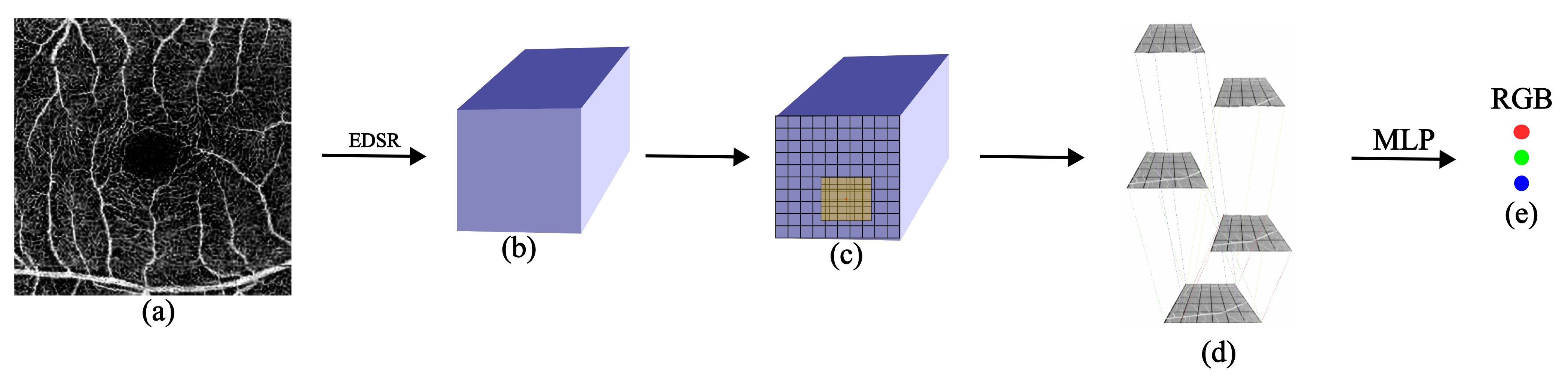
3. Method
3.1. Backbone Framework
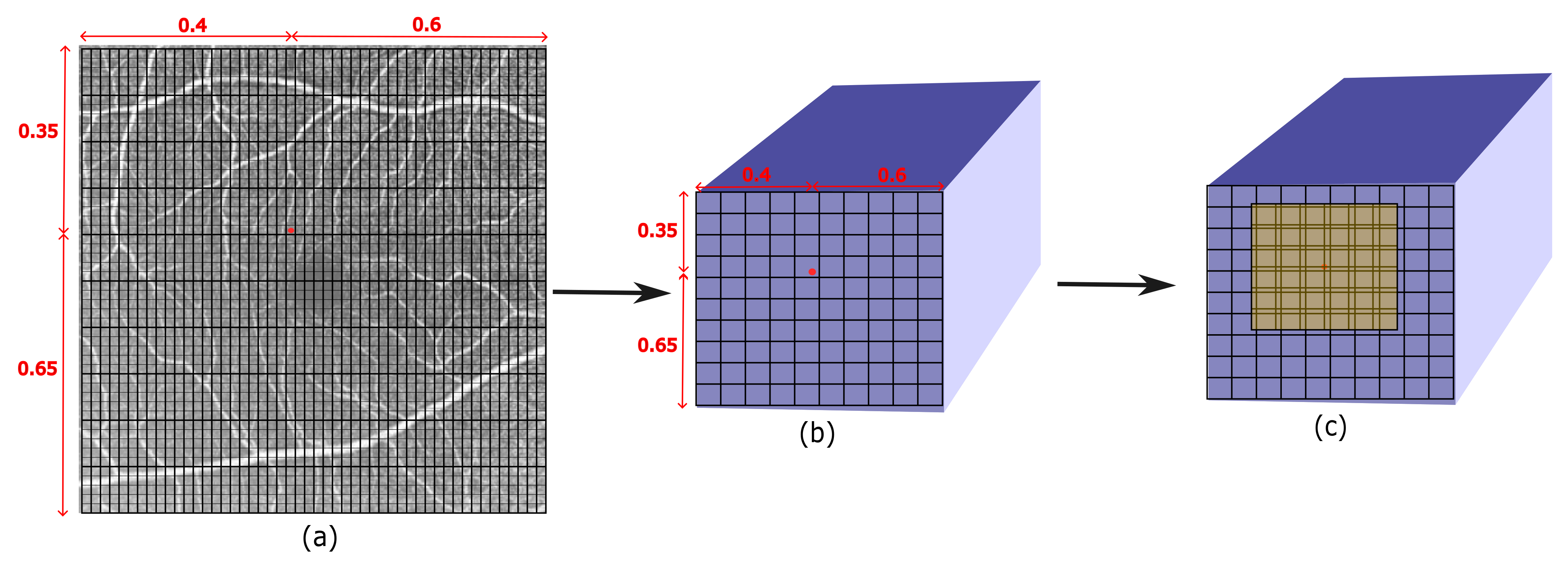
3.2. Locating the Semi-Local Region
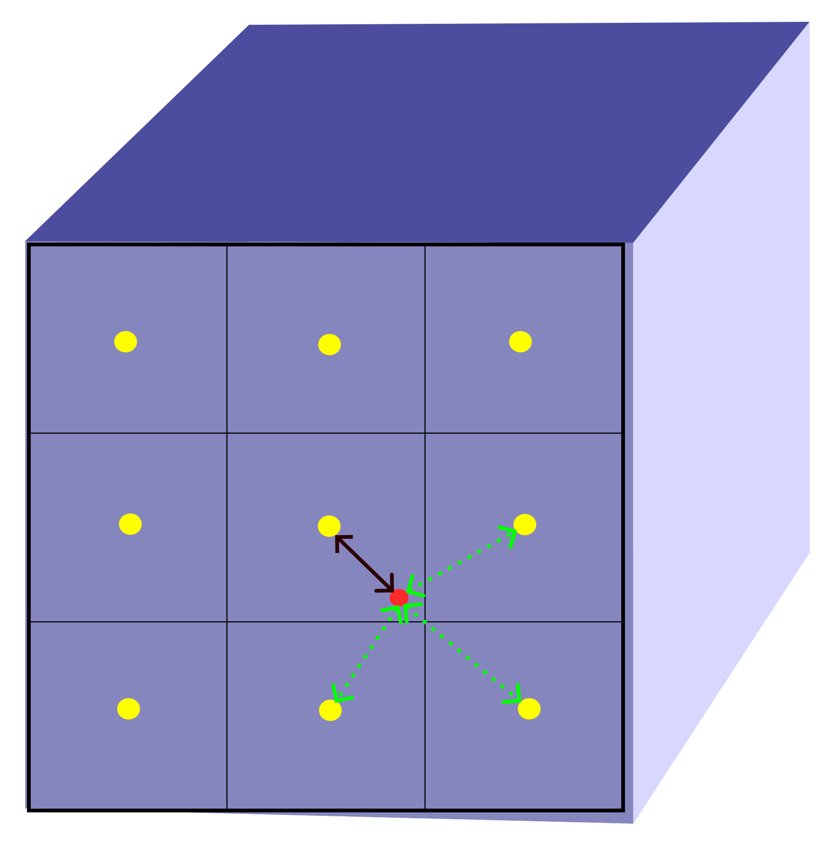
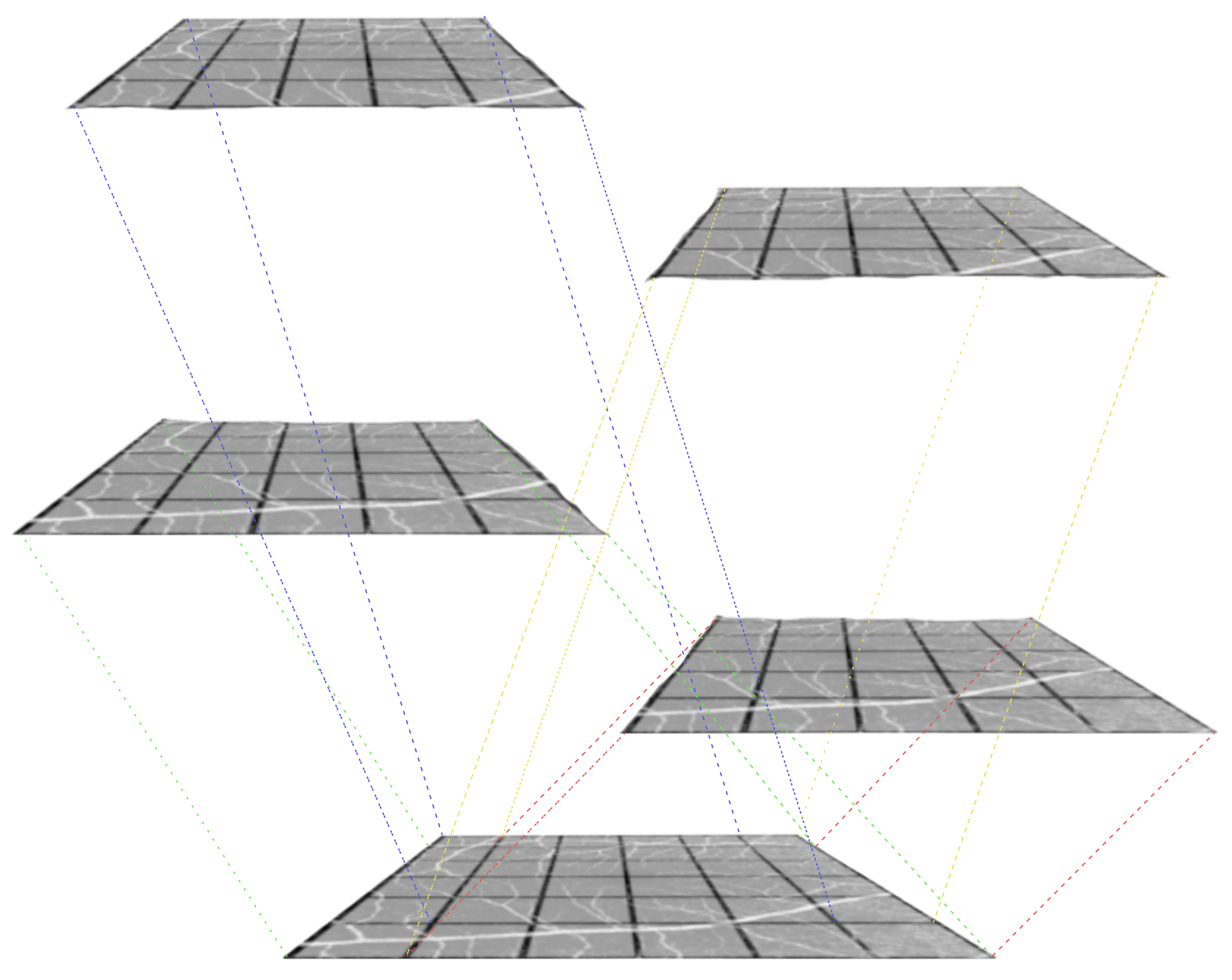
3.3. Overlapping Windows
4. Results and Discussion
4.1. Dataset
4.2. Implementation Details
4.3. Quantitative Results
5. Conclusions and Future Work
Author Contributions
Funding
Data Availability Statement
Conflicts of Interest
References
- Bashir, S.M.A.; Wang, Y.; Khan, M.; Niu, Y. A comprehensive review of deep learning based single image super-resolution. Peer J. Comput. Sci. 2021, 7, 1–56. [Google Scholar] [CrossRef] [PubMed]
- Tan, R.; Yuan, Y.; Huang, R.; Luo, J. Video super-resolution with spatial-temporal transformer encoder. In Proceedings of the IEEE International Conference on Multimedia and Expo (ICME), Taipei, Taiwan, 18–22 July 2022; pp. 1–6. [Google Scholar]
- Li, H.; Zhang, P. Spatio-temporal fusion network for video super-resolution. In Proceedings of the International Joint Conference on Neural Networks, Online, 18–22 July 2021. [Google Scholar]
- Thawakar, O.; Patil, P.W.; Dudhane, A.; Murala, S.; Kulkarni, U. Image and video super resolution using recurrent generative adversarial network. In Proceedings of the 16th IEEE International Conference on Advanced Video and Signal Based Surveillance AVSS 2019, Taipei, Taiwan, 18–21 September 2019. [Google Scholar]
- Li, H.; Yang, Y.; Chang, M.; Feng, H.; Xu, Z.; Li, Q.; Chen, Y. SRDiff: Single image super-resolution with diffusion probabilistic models. Neurocomputing 2022, 479, 47–59. [Google Scholar] [CrossRef]
- Girshick, R.; Donahue, J.; Darrell, T.; Malik, J. Region-based convolutional networks for accurate object detection and segmentation. IEEE Trans. Pattern. Anal. Mach. Intell. 2016, 38, 142–158. [Google Scholar] [CrossRef] [PubMed]
- Liang, J.; Cao, J.; Sun, G.; Zhang, K.; Van Gool, L.; Timofte, R.S. Image restoration using swin transformer. In Proceedings of the IEEE/CVF international Conference on Computer Vision, Montreal, BC, Canada, 11–17 October 2021; pp. 1833–1844. [Google Scholar]
- Shi, W.; Jose, C.; Ferenc, H.; Johannes, T.; Andrew, A.P.; Rob, B.; Daniel, R.; Wang, Z. Real-time single image and video super-resolution using an efficient sub-pixel convolutional neural network. In Proceedings of the IEEE Conference on Computer Vision and Pattern Recognition, Las Vegas, NV, USA, 27–30 June 2016; pp. 1874–1883. [Google Scholar]
- Zhang, Y.; Li, K.; Li, K.; Wang, L.; Zhong, B.; Fu, Y. Image super-resolution using very deep residual channel attention networks. In Proceedings of the European Conference on Computer Vision (ECCV), Munich, Germany, 8–14 September 2018; pp. 286–301. [Google Scholar]
- Peng, S.; Niemeyer, M.; Mescheder, L.; Pollefeys, M.; Geiger, A. Convolutional Occupancy Networks. In Proceedings of the Computer Vision–ECCV 2020: 16th European Conference, Glasgow, UK, 23–28 August 2020; pp. 523–540. [Google Scholar]
- Lim, B.; Son, S.; Kim, H.; Nah, S.; Mu Lee, K. Enhanced deep residual networks for single image super-resolution. In Proceedings of the IEEE Conference on Computer Vision and Pattern Recognition Workshops, Honolulu, HI, USA, 21–26 July 2017; pp. 136–144. [Google Scholar]
- Saito, S.; Huang, Z.; Natsume, R.; Morishima, S.; Kanazawa, A.; Li, H. Pifu: Pixel-aligned implicit function for high-resolution clothed human digitization. In Proceedings of the IEEE/CVF International Conference on Computer Vision, Seoul, Republic of Korea, 27 October–2 November 2019; pp. 2304–2314. [Google Scholar]
- Park, J.J.; Florence, P.; Straub, J.; Newcombe, R.; Lovegrove, S. Deepsdf: Learning continuous signed distance functions for shape representation. In Proceedings of the IEEE/CVF Conference on Computer Vision and Pattern Recognition, Long Beach, CA, USA, 15–20 June 2019; pp. 165–174. [Google Scholar]
- Mescheder, L.; Oechsle, M.; Niemeyer, M.; Nowozin, S.; Geiger, A. Occupancy networks: Learning 3d reconstruction in function space. In Proceedings of the IEEE/CVF Conference on Computer Vision and Pattern Recognition, Long Beach, CA, USA, 15–20 June 2019; pp. 4460–4470. [Google Scholar]
- Sitzmann, V.; Martel, J.; Bergman, A.; Lindell, D.; Wetzstein, G. Implicit neural representations with periodic activation functions. Adv. Neural Inf. Process. Syst. 2020, 33, 7462–7473. [Google Scholar]
- Chen, Y.; Liu, S.; Wang, X. Learning continuous image representation with local implicit image function. In Proceedings of the IEEE/CVF Conference on Computer Vision and Pattern Recognition, Nashville, TN, USA, 20–25 June 2021; pp. 8628–8638. [Google Scholar]
- Dong, C.; Loy, C.C.; He, K.; Tang, X. Image super-resolution using deep convolutional networks. IEEE Trans. Pattern Anal. Mach. Intell. 2015, 38, 295–307. [Google Scholar] [CrossRef] [PubMed]
- Kim, J.; Lee, J.K.; Lee, K.M. Accurate image super-resolution using very deep convolutional networks. In Proceedings of the IEEE Conference on Computer Vision and Pattern Recognition, Las Vegas, NV, USA, 27–30 June 2016; pp. 1646–1654. [Google Scholar]
- Ledig, C.; Theis, L.; Huszár, F.; Caballero, J.; Cunningham, A.; Acosta, A.; Aitken, A.; Tejani, A.; Totz, J.; Wang, Z.; et al. Photo-realistic single image super-resolution using a generative adversarial network. In Proceedings of the IEEE Conference on Computer Vision and Pattern Recognition, Honolulu, HI, USA, 21–26 July 2017; pp. 4681–4690. [Google Scholar]
- Mei, Y.; Fan, Y.; Zhou, Y. Image super-resolution with non-local sparse attention. In Proceedings of the IEEE/CVF Conference on Computer Vision and Pattern Recognition, Nashville, TN, USA, 20–25 June 2021; pp. 3517–3526. [Google Scholar]
- Zhang, Y.; Tian, Y.; Kong, Y.; Zhong, B.; Fu, Y. Residual dense network for image super-resolution. In Proceedings of the IEEE Conference on Computer Vision and Pattern Recognition, Salt Lake City, UT, USA, 18–23 June 2018; pp. 2472–2481. [Google Scholar]
- Sajjadi, M.S.M.; Scholkopf, B.; Hirsch, M. Enhancenet: Single image super-resolution through automated texture synthesis. In Proceedings of the IEEE International Conference on Computer Vision, Venice, Italy, 22–29 October 2017; pp. 4491–4500. [Google Scholar]
- Wang, X.; Yu, K.; Dong, C.; Loy, C.C. Recovering realistic texture in image super-resolution by deep spatial feature transform. In Proceedings of the IEEE Conference on Computer Vision and Pattern Recognition, Salt Lake City, UT, USA, 18–23 June 2018; pp. 606–615. [Google Scholar]
- Wang, X.; Yu, K.; Wu, S.; Gu, J.; Liu, Y.; Dong, C.; Qiao, Y.; Chen, C.L.; Qiao, Y.; Tang, X. Esrgan: Enhanced super-resolution generative adversarial networks. In Proceedings of the European Conference on Computer Vision (ECCV) Workshops, Munich, Germany, 8–14 September 2018. [Google Scholar]
- Wang, X.; Xie, L.; Dong, C.; Shan, Y. Real-esrgan: Training real-world blind super-resolution with pure synthetic data. In Proceedings of the IEEE/CVF International Conference on Computer Vision, Montreal, BC, Canada, 11–17 October 2021; pp. 1905–1914. [Google Scholar]
- Li, M.; Chen, Y.; Yuan, S.; Chen, Q. OCTA-500. 2019. Available online: https://arxiv.org/ftp/arxiv/papers/2012/2012.07261.pdf (accessed on 23 October 2023).
- Adam, P.; Sam, G.; Francisco, M.; Adam, L.; James, B.; Gregory, C.; Trevor, K.; Lin, Z.; Natalia, G.; Luca, A.; et al. PyTorch: An Imperative Style, High-Performance Deep Learning Library. In Advances in Neural Information Processing Systems; Curran Associates, Inc.: Red Hook, NY, USA, 2019; Volume 32. [Google Scholar]
- Kingma, D.P.; Ba, J.A. A method for stochastic optimization. arXiv 2014, arXiv:1412.6980. [Google Scholar]


| Patch Size | Bicubic | SRCNN [17] | EDSR [11] | OW-SLR (Ours) |
|---|---|---|---|---|
| 24 × 24 | 11.96 | 12.87 | 13.79 | 13.92 |
| 32 × 32 | 14.18 | 15.10 | 16.04 | 16.26 |
| 48 × 48 | 15.37 | 16.89 | 17.66 | 17.98 |
| Extrapolation Factor | Time Taken (In Seconds) |
|---|---|
| 2× | 6.48 |
| 2.4× | 8.90 |
| 3× | 12.01 |
| 3.9× | 19.46 |
| 4.5× | 26.29 |
| 5× | 33.75 |
Disclaimer/Publisher’s Note: The statements, opinions and data contained in all publications are solely those of the individual author(s) and contributor(s) and not of MDPI and/or the editor(s). MDPI and/or the editor(s) disclaim responsibility for any injury to people or property resulting from any ideas, methods, instructions or products referred to in the content. |
© 2023 by the authors. Licensee MDPI, Basel, Switzerland. This article is an open access article distributed under the terms and conditions of the Creative Commons Attribution (CC BY) license (https://creativecommons.org/licenses/by/4.0/).
Share and Cite
Bhardwaj, R.; Jothi Balaji, J.; Lakshminarayanan, V. OW-SLR: Overlapping Windows on Semi-Local Region for Image Super-Resolution. J. Imaging 2023, 9, 246. https://doi.org/10.3390/jimaging9110246
Bhardwaj R, Jothi Balaji J, Lakshminarayanan V. OW-SLR: Overlapping Windows on Semi-Local Region for Image Super-Resolution. Journal of Imaging. 2023; 9(11):246. https://doi.org/10.3390/jimaging9110246
Chicago/Turabian StyleBhardwaj, Rishav, Janarthanam Jothi Balaji, and Vasudevan Lakshminarayanan. 2023. "OW-SLR: Overlapping Windows on Semi-Local Region for Image Super-Resolution" Journal of Imaging 9, no. 11: 246. https://doi.org/10.3390/jimaging9110246
APA StyleBhardwaj, R., Jothi Balaji, J., & Lakshminarayanan, V. (2023). OW-SLR: Overlapping Windows on Semi-Local Region for Image Super-Resolution. Journal of Imaging, 9(11), 246. https://doi.org/10.3390/jimaging9110246