
No-Reference Quality Assessment of Authentically Distorted Images Based on Local and Global Features


Abstract
:1. Introduction
2. Literature Review
3. Materials and Methods
3.1. Materials
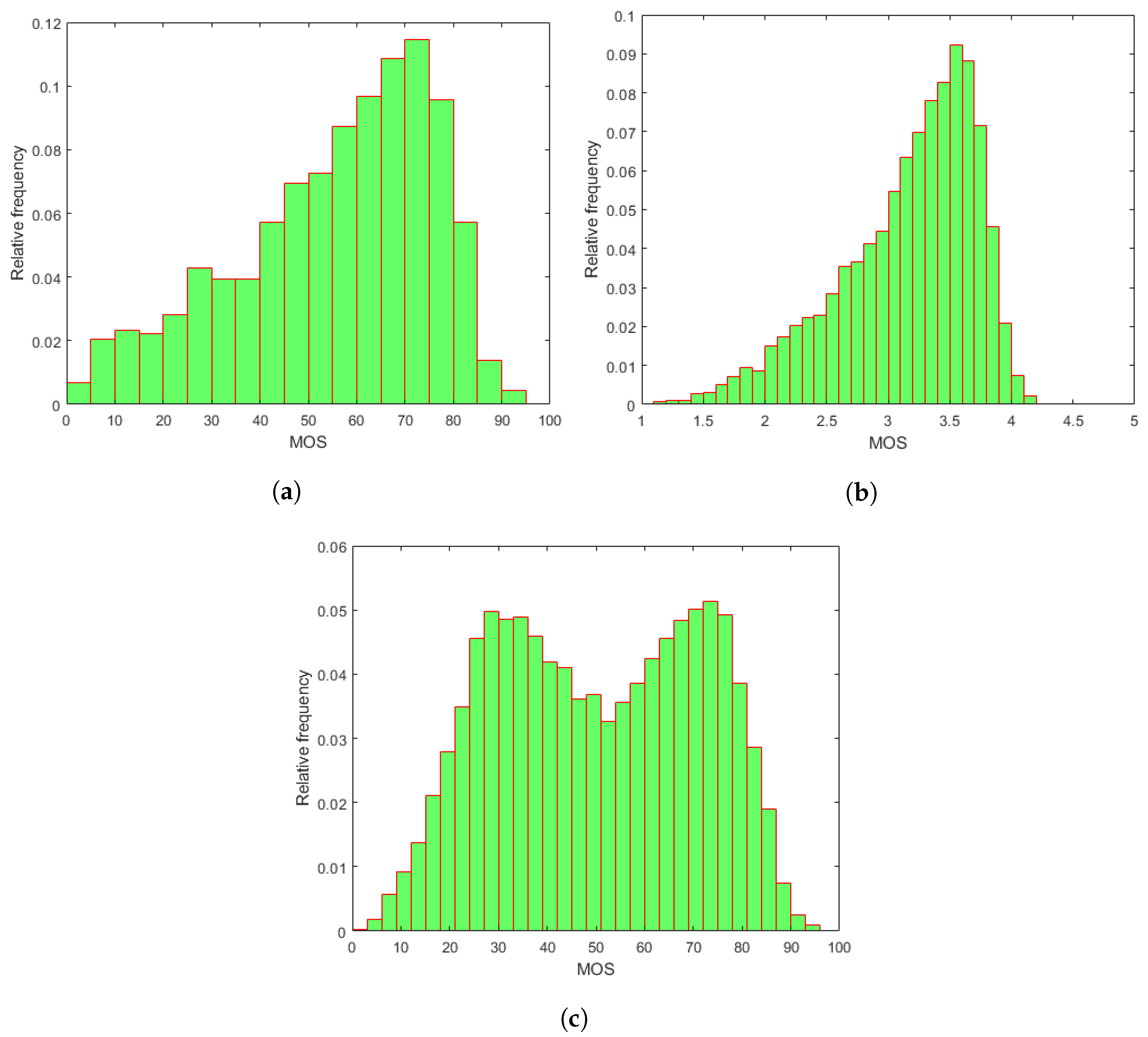
3.1.1. Applied IQA Databases
3.1.2. Evaluation
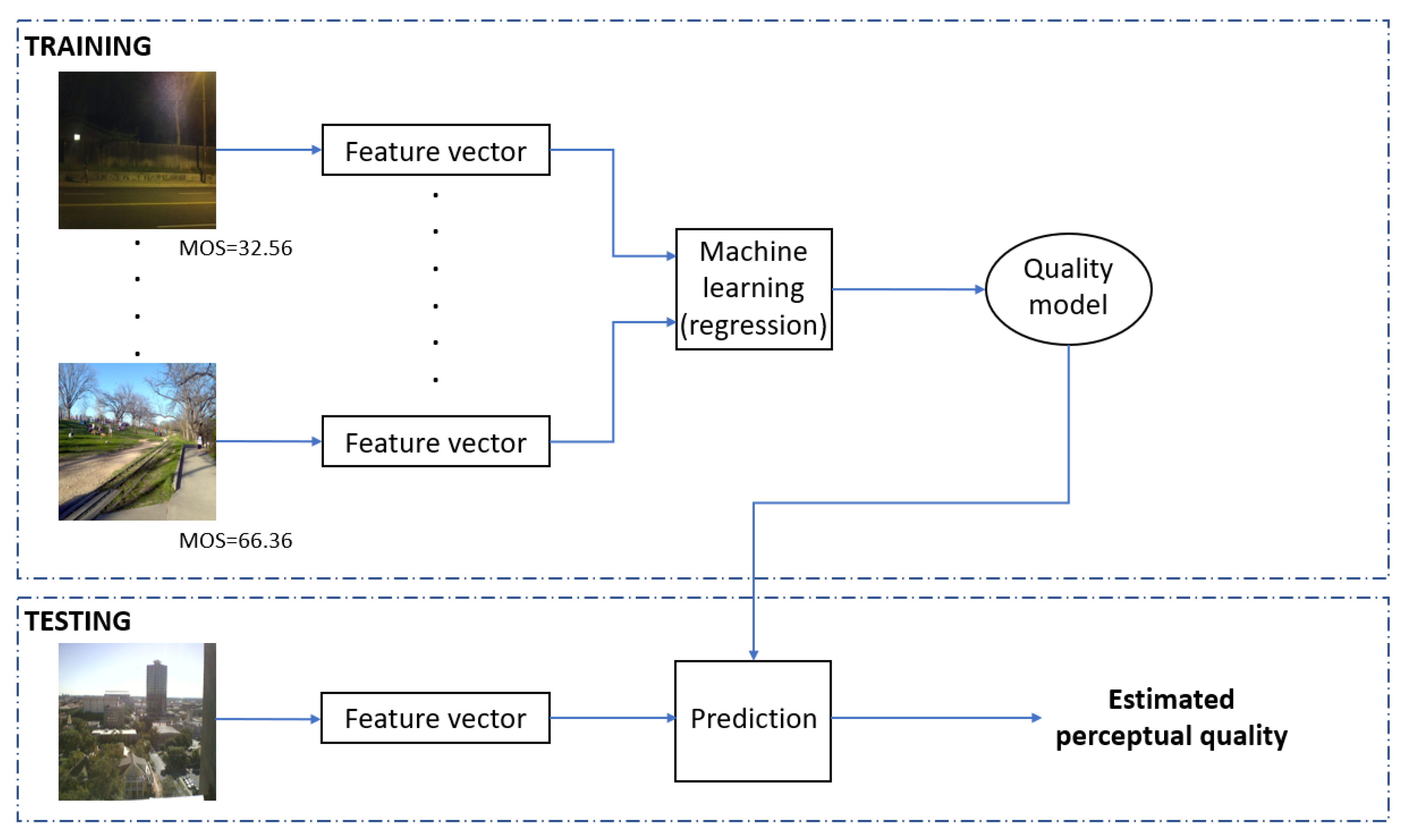
3.2. Methods

| Feature Number | Input | Feature | Number of Features |
|---|---|---|---|
| f1-f5 | SURF [55], Grayscale image | mean, median, std, skewness, kurtosis | 5 |
| f6-f10 | FAST [53], Grayscale image | mean, median, std, skewness, kurtosis | 5 |
| f11-f15 | BRISK [56], Grayscale image | mean, median, std, skewness, kurtosis | 5 |
| f16-f20 | KAZE [57], Grayscale image | mean, median, std, skewness, kurtosis | 5 |
| f21-f25 | ORB [58], Grayscale image | mean, median, std, skewness, kurtosis | 5 |
| f26-f30 | Harris [54], Grayscale image | mean, median, std, skewness, kurtosis | 5 |
| f31-f35 | Minimum Eigenvalue [59], Grayscale image | mean, median, std, skewness, kurtosis | 5 |
| f36-f40 | SURF [55], Filtered image | mean, median, std, skewness, kurtosis | 5 |
| f41-f45 | FAST [53], Filtered image | mean, median, std, skewness, kurtosis | 5 |
| f46-f50 | BRISK [56], Filtered image | mean, median, std, skewness, kurtosis | 5 |
| f51-f55 | KAZE [57], Filtered image | mean, median, std, skewness, kurtosis | 5 |
| f56-f60 | ORB [58], Filtered image | mean, median, std, skewness, kurtosis | 5 |
| f61-f65 | Harris [54], Filtered image | mean, median, std, skewness, kurtosis | 5 |
| f66-f70 | Minimum Eigenvalue [59], Filtered image | mean, median, std, skewness, kurtosis | 5 |
| f71-f77 | Binary image | Hu invariant moments [60] | 7 |
| f78-f87 | RGB image | Perceptual features | 10 |
| f88 | GL-GM map | histogram variance | 1 |
| f89 | GL-GM map | histogram variance | 1 |
| f90 | GL-GM map | histogram variance | 1 |
| f91 | GM map [61] | histogram variance | 1 |
| f92 | RO map [61] | histogram variance | 1 |
| f93 | RM map [61] | histogram variance | 1 |
3.3. Statistics of Local Feature Descriptors
3.4. Hu Invariant Moments
3.5. Perceptual Features
- Blur: It is probably the most dominant source of perceptual image quality deterioration in digital imaging [67]. To quantify the emergence of the blur effect, the blur metric of Crété-Roffet et al. [68], which is based on the measurements of intensity variations between neighboring pixels, was implemented due to its low computational costs.
- Colorfulness: In [69], Choi et al. pointed out that colorfulness is a critical component in human image quality judgment. We determined colorfulness using the following formula proposed by Hasler and Suesstrunk [70]:where and stand for the standard deviation and the mean of the matrices denoted in the subscripts, respectively. Specifically, these matrices are given as:where R, G, and B are the red, green, and blue color channels, respectively.
- Chroma: It is one of the relevant image features among a series of color metrics in the CIELAB color space. Moreover, chroma is significantly correlated with haze, blur, or motion blur in the image [70]. It is defined aswhere a and b are the corresponding color channels of the CIELAB color space. The arithmetic mean of was used as a perceptual feature in our model.
- Color gradient: The estimated color gradient magnitude (CGM) map is defined aswhere and stand for the approximate directional derivatives in the horizontal x and vertical y directions of , respectively. In our study, the mean and standard deviations of are utilized as quality-aware features.
- Dark channel feature (DCF): In the literature, Tang et al. [71] proposed DCF [72] for image quality assessment, since it can effectively identify haze effects in images. A dark channel is defined aswhere denotes the image patches around the pixel location x. In our implementation, an image patch corresponds to a square. Next, the DCF is defined aswhere is the size of image I.
- Michelson contrast: Contrast is one of the most fundamental characteristics of an image, since it influences the ability to distinguish objects from each other in an image [73]. Thus, contrast information is built into our NR-IQA model. The Michelson contrast measures the difference between the maximum and minimum values of an image [74], defined as
- Root mean square (RMS) contrast is defined aswhere denotes the mean luminance of .
- Global contrast factor (GCF): Contrary to Michelson and RMS contrasts, GCF considers multiple resolution levels of an image to estimate human contrast perception [75]. It is defined aswhere ’s are the average local contrasts and ’s are the weighting factors. The authors examined nine different resolution levels, which is why the number of weighting factors are nine; ’s are defined aswhich is a result of an optimum approximation from the best fitting [75]. The local contrasts are defined as follows. First, the image of size is rearranged into a one-dimensional vector using row-wise sorting. Next, the local contrast in pixel location i is defined aswhere denotes the pixel value at location i after gamma correction . Finally, the average local contrast at resolution i (denoted by in Equation (31)) is determined as the average of all ’s over the entire image.
- Entropy: It is a quantitative measure of the image’s carried information [76]. Typically, an image with better quality is able to transmit more information. This is why entropy was chosen as a quality-aware feature. The entropy of a grayscale image is defined aswhere consists of the normalized histogram counts of the grayscale image.
3.6. Relative Grünwald–Letnikov Derivative and Gradient Statistics
4. Results
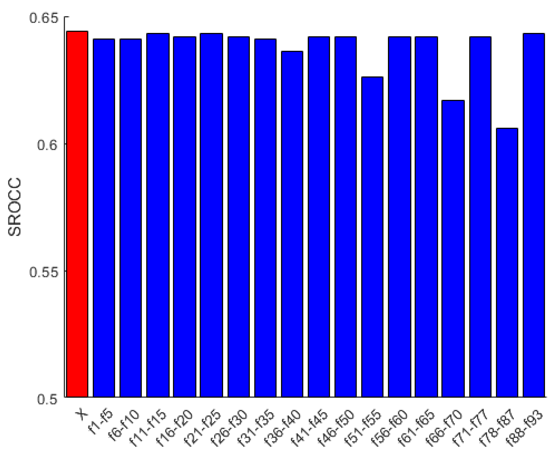
4.1. Ablation Study
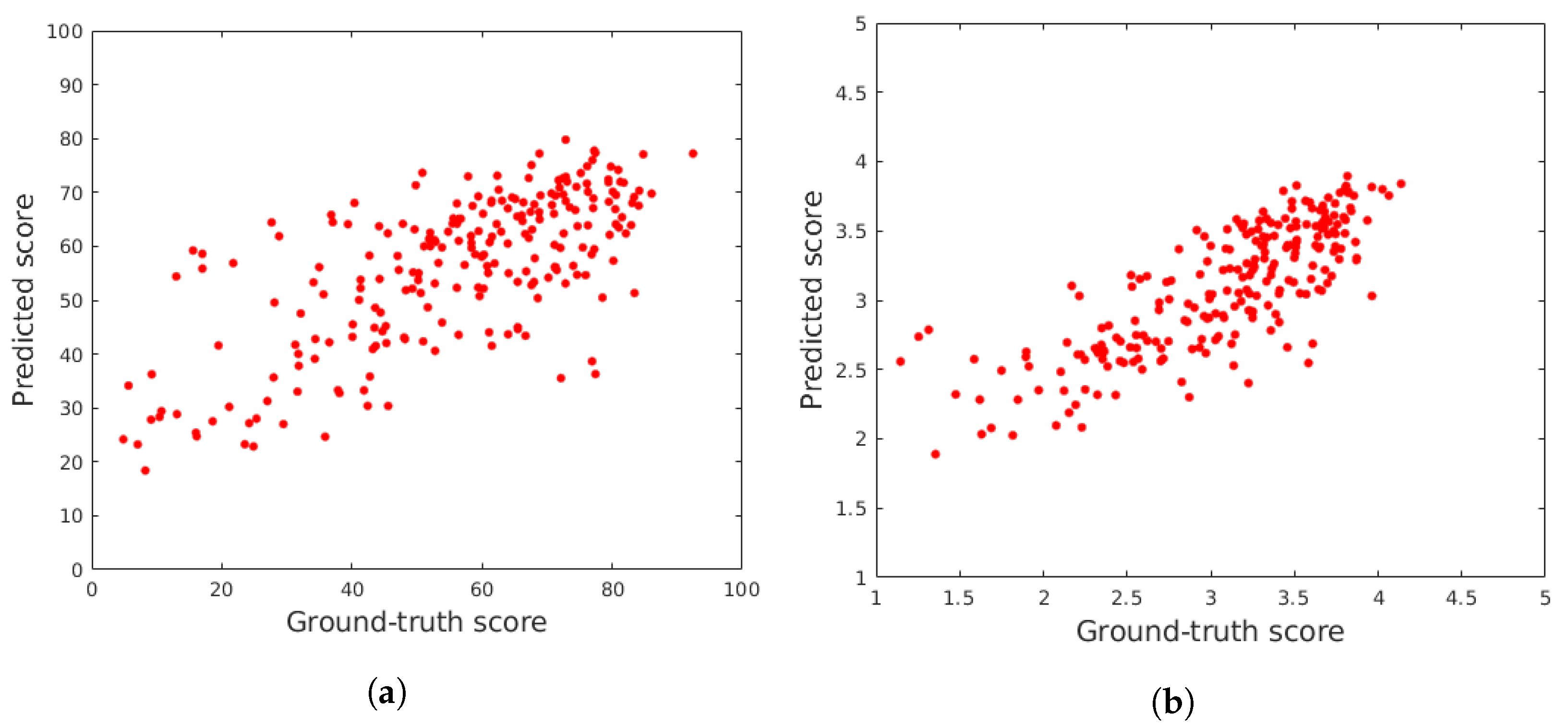
4.2. Comparison to the State-of-the-Art
5. Conclusions
Funding
Institutional Review Board Statement
Informed Consent Statement
Data Availability Statement
Acknowledgments
Conflicts of Interest
Abbreviations
| BRIEF | binary robust independent elementary features |
| BRISK | binary robust invariant scalable keypoints |
| CGM | color gradient magnitude |
| CNN | convolutional neural network |
| CPU | central processing unit |
| DCF | dark channel feature |
| DCT | discrete cosine transform |
| DF | decision fusion |
| DSC | digital still camera |
| DSLR | digital single-lens reflex camera |
| FAST | features from accelerated segment test |
| FR | full-reference |
| GGD | generalized Gaussian distribution |
| GL | Grünwald–Letnikov |
| GM | gradient magnitude |
| GPU | graphics processing unit |
| GPR | Gaussian process regression |
| IQA | image quality assessment |
| KROCC | Kendall’s rank-order correlation coefficient |
| MOS | mean opinion score |
| MSCN | mean subtracted contrast normalized |
| NIQE | naturalness image quality evaluator |
| NR | no-reference |
| NSS | natural scene statistics |
| ORB | oriented FAST and rotated BRIEF |
| PIQE | perception-based image quality evaluator |
| PLCC | Pearson’s linear correlation coefficient |
| RBF | radial basis function |
| RM | relative gradient magnitude |
| RMS | root mean square |
| RO | relative gradient orientation |
| RR | reduced-reference |
| SPHN | smartphone |
| SROCC | Spearman’s rank-order correlation coefficient |
| SVR | support vector regressor |
References
- Torr, P.H.; Zissermann, A. Performance characterization of fundamental matrix estimation under image degradation. Mach. Vis. Appl. 1997, 9, 321–333. [Google Scholar] [CrossRef]
- Zhao, Q. The Application of Augmented Reality Visual Communication in Network Teaching. Int. J. Emerg. Technol. Learn. 2018, 13, 57. [Google Scholar] [CrossRef]
- Shen, T.W.; Li, C.C.; Lin, W.F.; Tseng, Y.H.; Wu, W.F.; Wu, S.; Tseng, Z.L.; Hsu, M.H. Improving Image Quality Assessment Based on the Combination of the Power Spectrum of Fingerprint Images and Prewitt Filter. Appl. Sci. 2022, 12, 3320. [Google Scholar] [CrossRef]
- Esteban, O.; Birman, D.; Schaer, M.; Koyejo, O.O.; Poldrack, R.A.; Gorgolewski, K.J. MRIQC: Advancing the automatic prediction of image quality in MRI from unseen sites. PLoS ONE 2017, 12, e0184661. [Google Scholar] [CrossRef] [PubMed] [Green Version]
- Ma, K.; Yeganeh, H.; Zeng, K.; Wang, Z. High dynamic range image compression by optimizing tone mapped image quality index. IEEE Trans. Image Process. 2015, 24, 3086–3097. [Google Scholar]
- Goyal, B.; Gupta, A.; Dogra, A.; Koundal, D. An adaptive bitonic filtering based edge fusion algorithm for Gaussian denoising. Int. J. Cogn. Comput. Eng. 2022, 3, 90–97. [Google Scholar] [CrossRef]
- Zhai, G.; Min, X. Perceptual image quality assessment: A survey. Sci. China Inf. Sci. 2020, 63, 1–52. [Google Scholar] [CrossRef]
- Kamble, V.; Bhurchandi, K. No-reference image quality assessment algorithms: A survey. Optik 2015, 126, 1090–1097. [Google Scholar] [CrossRef]
- Mittal, A.; Moorthy, A.K.; Bovik, A.C. No-reference image quality assessment in the spatial domain. IEEE Trans. Image Process. 2012, 21, 4695–4708. [Google Scholar] [CrossRef]
- Liu, L.; Dong, H.; Huang, H.; Bovik, A.C. No-reference image quality assessment in curvelet domain. Signal Process. Image Commun. 2014, 29, 494–505. [Google Scholar] [CrossRef]
- Xue, W.; Mou, X.; Zhang, L.; Bovik, A.C.; Feng, X. Blind image quality assessment using joint statistics of gradient magnitude and Laplacian features. IEEE Trans. Image Process. 2014, 23, 4850–4862. [Google Scholar] [CrossRef] [PubMed]
- Min, X.; Zhai, G.; Gu, K.; Liu, Y.; Yang, X. Blind image quality estimation via distortion aggravation. IEEE Trans. Broadcast. 2018, 64, 508–517. [Google Scholar] [CrossRef]
- Mohammadi, P.; Ebrahimi-Moghadam, A.; Shirani, S. Subjective and objective quality assessment of image: A survey. arXiv 2014, arXiv:1406.7799. [Google Scholar]
- Yang, X.; Li, F.; Liu, H. A survey of DNN methods for blind image quality assessment. IEEE Access 2019, 7, 123788–123806. [Google Scholar] [CrossRef]
- Xu, L.; Lin, W.; Kuo, C.C.J. Visual Quality Assessment by Machine Learning; Springer: Berlin/Heidelberg, Germany, 2015. [Google Scholar]
- Venkatanath, N.; Praneeth, D.; Bh, M.C.; Channappayya, S.S.; Medasani, S.S. Blind image quality evaluation using perception based features. In Proceedings of the 2015 Twenty First National Conference on Communications (NCC), Bombay, India, 27 February–1 March 2015; pp. 1–6. [Google Scholar]
- Mittal, A.; Soundararajan, R.; Bovik, A.C. Making a “completely blind” image quality analyzer. IEEE Signal Process. Lett. 2012, 20, 209–212. [Google Scholar] [CrossRef]
- Zhang, L.; Zhang, L.; Bovik, A.C. A feature-enriched completely blind image quality evaluator. IEEE Trans. Image Process. 2015, 24, 2579–2591. [Google Scholar] [CrossRef] [Green Version]
- Wu, L.; Zhang, X.; Chen, H.; Wang, D.; Deng, J. VP-NIQE: An opinion-unaware visual perception natural image quality evaluator. Neurocomputing 2021, 463, 17–28. [Google Scholar] [CrossRef]
- Bhattacharyya, A. On a measure of divergence between two statistical populations defined by their probability distributions. Bull. Calcutta Math. Soc. 1943, 35, 99–109. [Google Scholar]
- Leonardi, M.; Napoletano, P.; Schettini, R.; Rozza, A. No Reference, Opinion Unaware Image Quality Assessment by Anomaly Detection. Sensors 2021, 21, 994. [Google Scholar] [CrossRef]
- Reinagel, P.; Zador, A.M. Natural scene statistics at the centre of gaze. Netw. Comput. Neural Syst. 1999, 10, 341. [Google Scholar] [CrossRef]
- Saad, M.A.; Bovik, A.C.; Charrier, C. Blind image quality assessment: A natural scene statistics approach in the DCT domain. IEEE Trans. Image Process. 2012, 21, 3339–3352. [Google Scholar] [CrossRef] [PubMed]
- Moorthy, A.K.; Bovik, A.C. A two-step framework for constructing blind image quality indices. IEEE Signal Process. Lett. 2010, 17, 513–516. [Google Scholar] [CrossRef]
- Moorthy, A.K.; Bovik, A.C. Blind image quality assessment: From natural scene statistics to perceptual quality. IEEE Trans. Image Process. 2011, 20, 3350–3364. [Google Scholar] [CrossRef] [PubMed]
- Tang, H.; Joshi, N.; Kapoor, A. Learning a blind measure of perceptual image quality. In Proceedings of the CVPR 2011, Colorado Springs, CO, USA, 20–25 June 2011; pp. 305–312. [Google Scholar]
- Wang, Q.; Chu, J.; Xu, L.; Chen, Q. A new blind image quality framework based on natural color statistic. Neurocomputing 2016, 173, 1798–1810. [Google Scholar] [CrossRef]
- Wu, J.; Lin, W.; Shi, G. Image quality assessment with degradation on spatial structure. IEEE Signal Process. Lett. 2014, 21, 437–440. [Google Scholar] [CrossRef]
- Freitas, P.G.; Akamine, W.Y.; Farias, M.C. No-reference image quality assessment based on statistics of local ternary pattern. In Proceedings of the 2016 Eighth International Conference on Quality of Multimedia Experience (QoMEX), Lisbon, Portugal, 6–8 June 2016; pp. 1–6. [Google Scholar]
- Freitas, P.G.; Akamine, W.Y.; Farias, M.C. No-reference image quality assessment using orthogonal color planes patterns. IEEE Trans. Multimed. 2018, 20, 3353–3360. [Google Scholar] [CrossRef]
- Ojala, T.; Pietikäinen, M.; Harwood, D. A comparative study of texture measures with classification based on featured distributions. Pattern Recognit. 1996, 29, 51–59. [Google Scholar] [CrossRef]
- Garcia Freitas, P.; Da Eira, L.P.; Santos, S.S.; Farias, M.C.Q.d. On the Application LBP Texture Descriptors and Its Variants for No-Reference Image Quality Assessment. J. Imaging 2018, 4, 114. [Google Scholar] [CrossRef] [Green Version]
- Ye, P.; Doermann, D. No-reference image quality assessment based on visual codebook. In Proceedings of the 2011 18th IEEE International Conference on Image Processing, Brussels, Belgium, 11–14 September 2011; pp. 3089–3092. [Google Scholar]
- Ye, P.; Doermann, D. No-reference image quality assessment using visual codebooks. IEEE Trans. Image Process. 2012, 21, 3129–3138. [Google Scholar]
- Ye, P.; Kumar, J.; Kang, L.; Doermann, D. Unsupervised feature learning framework for no-reference image quality assessment. In Proceedings of the 2012 IEEE Conference on Computer Vision and Pattern Recognition, Providence, RI, USA, 16–21 June 2012; pp. 1098–1105. [Google Scholar]
- Kang, L.; Ye, P.; Li, Y.; Doermann, D. Convolutional neural networks for no-reference image quality assessment. In Proceedings of the IEEE Conference on Computer Vision and Pattern Recognition, Columbus, OH, USA, 23–28 June 2014; pp. 1733–1740. [Google Scholar]
- Bianco, S.; Celona, L.; Napoletano, P.; Schettini, R. On the use of deep learning for blind image quality assessment. Signal Image Video Process. 2018, 12, 355–362. [Google Scholar] [CrossRef] [Green Version]
- Gao, F.; Yu, J.; Zhu, S.; Huang, Q.; Tian, Q. Blind image quality prediction by exploiting multi-level deep representations. Pattern Recognit. 2018, 81, 432–442. [Google Scholar] [CrossRef]
- Yang, S.; Jiang, Q.; Lin, W.; Wang, Y. Sgdnet: An end-to-end saliency-guided deep neural network for no-reference image quality assessment. In Proceedings of the 27th ACM International Conference on Multimedia, Nice, France, 21–25 October 2019; pp. 1383–1391. [Google Scholar]
- Zhang, L.; Shen, Y.; Li, H. VSI: A visual saliency-induced index for perceptual image quality assessment. IEEE Trans. Image Process. 2014, 23, 4270–4281. [Google Scholar] [CrossRef] [PubMed] [Green Version]
- Liu, X.; Van De Weijer, J.; Bagdanov, A.D. Rankiqa: Learning from rankings for no-reference image quality assessment. In Proceedings of the IEEE International Conference on Computer Vision, Venice, Italy, 22–29 October 2017; pp. 1040–1049. [Google Scholar]
- Burges, C.; Shaked, T.; Renshaw, E.; Lazier, A.; Deeds, M.; Hamilton, N.; Hullender, G. Learning to rank using gradient descent. In Proceedings of the 22nd International Conference on Machine Learning, Bonn, Germany, 7–11 August 2005; pp. 89–96. [Google Scholar]
- Li, D.; Jiang, T.; Jiang, M. Norm-in-norm loss with faster convergence and better performance for image quality assessment. In Proceedings of the 28th ACM International Conference on Multimedia, Seattle, WA, USA, 12–16 October 2020; pp. 789–797. [Google Scholar]
- Celona, L.; Schettini, R. Blind quality assessment of authentically distorted images. JOSA A 2022, 39, B1–B10. [Google Scholar] [CrossRef]
- Ghadiyaram, D.; Bovik, A.C. Massive online crowdsourced study of subjective and objective picture quality. IEEE Trans. Image Process. 2015, 25, 372–387. [Google Scholar] [CrossRef] [PubMed] [Green Version]
- Lin, H.; Hosu, V.; Saupe, D. KonIQ-10K: Towards an ecologically valid and large-scale IQA database. arXiv 2018, arXiv:1803.08489. [Google Scholar]
- Fang, Y.; Zhu, H.; Zeng, Y.; Ma, K.; Wang, Z. Perceptual quality assessment of smartphone photography. In Proceedings of the IEEE/CVF Conference on Computer Vision and Pattern Recognition, Seattle, WA, USA, 13–19 June 2020; pp. 3677–3686. [Google Scholar]
- Guan, X.; Li, F.; He, L. Quality Assessment on Authentically Distorted Images by Expanding Proxy Labels. Electronics 2020, 9, 252. [Google Scholar] [CrossRef] [Green Version]
- Ding, Y. Visual Quality Assessment for Natural and Medical Image; Springer: Berlin/Heidelberg, Germany, 2018. [Google Scholar]
- Sheikh, H.R.; Sabir, M.F.; Bovik, A.C. A statistical evaluation of recent full reference image quality assessment algorithms. IEEE Trans. Image Process. 2006, 15, 3440–3451. [Google Scholar] [CrossRef]
- Varga, D. No-Reference Image Quality Assessment with Global Statistical Features. J. Imaging 2021, 7, 29. [Google Scholar] [CrossRef]
- Krig, S. Computer Vision Metrics; Springer: Berlin/Heidelberg, Germany, 2016. [Google Scholar]
- Rosten, E.; Drummond, T. Fusing points and lines for high performance tracking. In Proceedings of the Tenth IEEE International Conference on Computer Vision (ICCV’05) Volume 1, Beijing, China, 17–21 October 2005; Volume 2, pp. 1508–1515. [Google Scholar]
- Harris, C.; Stephens, M. A combined corner and edge detector. In Proceedings of the Alvey Vision Conference, Manchester, UK, 31 August–2 September 1988; Volume 15, pp. 10–5244. [Google Scholar]
- Bay, H.; Tuytelaars, T.; Gool, L.V. Surf: Speeded up robust features. In Proceedings of the European Conference on Computer Vision, Graz, Austria, 7–13 May 2006; pp. 404–417. [Google Scholar]
- Leutenegger, S.; Chli, M.; Siegwart, R.Y. BRISK: Binary robust invariant scalable keypoints. In Proceedings of the 2011 International Conference on Computer Vision, Las Vegas, NV, USA, 18–21 July 2011; pp. 2548–2555. [Google Scholar]
- Alcantarilla, P.F.; Bartoli, A.; Davison, A.J. KAZE features. In Proceedings of the European Conference on Computer Vision, Florence, Italy, 7–13 October 2012; pp. 214–227. [Google Scholar]
- Rublee, E.; Rabaud, V.; Konolige, K.; Bradski, G. ORB: An efficient alternative to SIFT or SURF. In Proceedings of the 2011 International Conference on Computer Vision, Las Vegas, NV, USA, 18–21 July 2011; pp. 2564–2571. [Google Scholar]
- Shi, J.; Tomasi. Good features to track. In Proceedings of the IEEE Conference on Computer Vision and Pattern Recognition, Seattle, WA, USA, 21–23 June 1994; pp. 593–600. [Google Scholar]
- Hu, M.K. Visual pattern recognition by moment invariants. IRE Trans. Inf. Theory 1962, 8, 179–187. [Google Scholar]
- Liu, L.; Hua, Y.; Zhao, Q.; Huang, H.; Bovik, A.C. Blind image quality assessment by relative gradient statistics and adaboosting neural network. Signal Process. Image Commun. 2016, 40, 1–15. [Google Scholar] [CrossRef]
- Moreno, P.; Bernardino, A.; Santos-Victor, J. Improving the SIFT descriptor with smooth derivative filters. Pattern Recognit. Lett. 2009, 30, 18–26. [Google Scholar] [CrossRef] [Green Version]
- Prewitt, J.M. Object enhancement and extraction. Pict. Process. Psychopictorics 1970, 10, 15–19. [Google Scholar]
- Marr, D.; Hildreth, E. Theory of edge detection. Proc. R. Soc. London Ser. B. Biol. Sci. 1980, 207, 187–217. [Google Scholar]
- Huang, J.S.; Tseng, D.H. Statistical theory of edge detection. Comput. Vis. Graph. Image Process. 1988, 43, 337–346. [Google Scholar] [CrossRef]
- Jenadeleh, M. Blind Image and Video Quality Assessment. Ph.D. Thesis, University of Konstanz, Konstanz, Germany, 2018. [Google Scholar]
- Kurimo, E.; Lepistö, L.; Nikkanen, J.; Grén, J.; Kunttu, I.; Laaksonen, J. The effect of motion blur and signal noise on image quality in low light imaging. In Proceedings of the Scandinavian Conference on Image Analysis, Oslo, Norway, 15–18 June; pp. 81–90.
- Crété-Roffet, F.; Dolmiere, T.; Ladret, P.; Nicolas, M. The blur effect: Perception and estimation with a new no-reference perceptual blur metric. In Proceedings of the SPIE Electronic Imaging Symposium Conf Human Vision and Electronic Imaging, San Jose, CA, USA, 29 January 29–1 February 2007. [Google Scholar]
- Choi, S.Y.; Luo, M.R.; Pointer, M.R.; Rhodes, P.A. Predicting perceived colorfulness, contrast, naturalness and quality for color images reproduced on a large display. In Proceedings of the Color and Imaging Conference, Society for Imaging Science and Technology, Portland, OR, USA, 10–14 November 2008; Volume 2008, pp. 158–164. [Google Scholar]
- Hasler, D.; Suesstrunk, S.E. Measuring colorfulness in natural images. In Proceedings of the Human Vision and Electronic Imaging VIII: International Society for Optics and Photonics, Santa Clara, CA, USA, 21–24 January 2003; Volume 5007, pp. 87–95. [Google Scholar]
- Tang, X.; Luo, W.; Wang, X. Content-based photo quality assessment. IEEE Trans. Multimed. 2013, 15, 1930–1943. [Google Scholar] [CrossRef] [Green Version]
- He, K.; Sun, J.; Tang, X. Single image haze removal using dark channel prior. IEEE Trans. Pattern Anal. Mach. Intell. 2010, 33, 2341–2353. [Google Scholar]
- Kukkonen, H.; Rovamo, J.; Tiippana, K.; Näsänen, R. Michelson contrast, RMS contrast and energy of various spatial stimuli at threshold. Vis. Res. 1993, 33, 1431–1436. [Google Scholar] [CrossRef]
- Michelson, A.A. Studies in Optics; Courier Corporation: Chelmsford, MA, USA, 1995. [Google Scholar]
- Matkovic, K.; Neumann, L.; Neumann, A.; Psik, T.; Purgathofer, W. Global contrast factor-a new approach to image contrast. In Proceedings of the Eurographics Workshop on Computational Aesthetics in Graphics, Visualization and Imaging 2005, Girona, Spain, 18–20 May 2005; pp. 159–167. [Google Scholar]
- Tsai, D.Y.; Lee, Y.; Matsuyama, E. Information entropy measure for evaluation of image quality. J. Digit. Imaging 2008, 21, 338–347. [Google Scholar] [CrossRef] [Green Version]
- Petrovic, V.S.; Xydeas, C.S. Gradient-based multiresolution image fusion. IEEE Trans. Image Process. 2004, 13, 228–237. [Google Scholar] [CrossRef]
- Dalal, N.; Triggs, B. Histograms of oriented gradients for human detection. In Proceedings of the 2005 IEEE Computer Society Conference on Computer Vision and Pattern Recognition (CVPR’05), San Diego, CA, USA, 20–25 June 2005; Volume 1, pp. 886–893. [Google Scholar]
- Kobayashi, T.; Otsu, N. Image feature extraction using gradient local auto-correlations. In Proceedings of the European Conference on Computer Vision, Marseille, France, 12–18 October 2008; pp. 346–358. [Google Scholar]
- Chiberre, P.; Perot, E.; Sironi, A.; Lepetit, V. Detecting Stable Keypoints from Events through Image Gradient Prediction. In Proceedings of the IEEE/CVF Conference on Computer Vision and Pattern Recognition, Nashville, TN, USA, 20–25 June 2021; pp. 1387–1394. [Google Scholar]
- Liu, A.; Lin, W.; Narwaria, M. Image quality assessment based on gradient similarity. IEEE Trans. Image Process. 2011, 21, 1500–1512. [Google Scholar]
- Gorenflo, R.; Mainardi, F. Fractional calculus. In Fractals and Fractional Calculus in Continuum Mechanics; Springer: Berlin/Heidelberg, Germany, 1997; pp. 223–276. [Google Scholar]
- Sabatier, J.; Agrawal, O.P.; Machado, J.T. Advances in Fractional Calculus; Springer: Berlin/Heidelberg, Germany, 2007; Volume 4. [Google Scholar]
- Motłoch, S.; Sarwas, G.; Dzieliński, A. Fractional Derivatives Application to Image Fusion Problems. Sensors 2022, 22, 1049. [Google Scholar] [CrossRef] [PubMed]
- Varga, D. Full-Reference Image Quality Assessment Based on Grünwald–Letnikov Derivative, Image Gradients, and Visual Saliency. Electronics 2022, 11, 559. [Google Scholar] [CrossRef]
- Robnik-Šikonja, M.; Kononenko, I. Theoretical and empirical analysis of ReliefF and RReliefF. Mach. Learn. 2003, 53, 23–69. [Google Scholar] [CrossRef] [Green Version]
- Kira, K.; Rendell, L.A. A practical approach to feature selection. In Machine Learning Proceedings 1992; Elsevier: Amsterdam, The Netherlands, 1992; pp. 249–256. [Google Scholar]
- Robnik-Šikonja, M.; Kononenko, I. An adaptation of Relief for attribute estimation in regression. In Proceedings of the Fourteenth International Conference on Machine Learning (ICML’97), San Francisco, CA, USA, 8–12 July 1997; Volume 5, pp. 296–304. [Google Scholar]
- Chen, X.; Zhang, Q.; Lin, M.; Yang, G.; He, C. No-reference color image quality assessment: From entropy to perceptual quality. EURASIP J. Image Video Process. 2019, 2019, 77. [Google Scholar] [CrossRef] [Green Version]
- Li, Q.; Lin, W.; Fang, Y. No-reference quality assessment for multiply-distorted images in gradient domain. IEEE Signal Process. Lett. 2016, 23, 541–545. [Google Scholar] [CrossRef]
- Ou, F.Z.; Wang, Y.G.; Zhu, G. A novel blind image quality assessment method based on refined natural scene statistics. In Proceedings of the 2019 IEEE International Conference on Image Processing (ICIP), Taipei, Taiwan, 22–29 September 2019; pp. 1004–1008. [Google Scholar]
- Liu, L.; Liu, B.; Huang, H.; Bovik, A.C. No-reference image quality assessment based on spatial and spectral entropies. Signal Process. Image Commun. 2014, 29, 856–863. [Google Scholar] [CrossRef]


| Attribute | CLIVE [45] | KonIQ-10k [46] | SPAQ [47] |
|---|---|---|---|
| #Images | 1162 | 10,073 | 11,125 |
| Resolution | |||
| #Subjects | 8100 | 1,467 | 600 |
| #Annotations | 1400 | 1,200,000 | 186,400 |
| Scale of quality scores | 0–100 | 1–5 | 0–100 |
| Subjective methodology | Crowdsourcing | Crowdsourcing | Laboratory |
| Types of cameras | DSLR/DSC/SPHN | DSLR/DSC/SPHN | SPHN |
| Year of publication | 2017 | 2018 | 2020 |
| Computer model | STRIX Z270H Gaming |
| Operating system | Windows 10 |
| CPU | Intel(R) Core(TM) i7-7700K CPU 4.20 GHz (8 cores) |
| Memory | 15 GB |
| GPU | Nvidia GeForce GTX 1080 |
| Blur | 0.412 | 0.362 | 0.315 | 0.285 | 0.329 |
| Colorfulness | 0.046 | 0.038 | 0.042 | 0.045 | 0.072 |
| Chroma | 15.510 | 13.681 | 14.995 | 15.409 | 21.977 |
| Color gradient-mean | 92.801 | 116.884 | 154.651 | 189.795 | 196.287 |
| Color gradient-std | 132.693 | 163.876 | 207.837 | 244.420 | 235.855 |
| DCF | 0.217 | 0.211 | 0.197 | 0.220 | 0.192 |
| Michelson contrast | 2.804 | 2.832 | 2.911 | 2.937 | 2.953 |
| RMS contrast | 0.201 | 0.201 | 0.219 | 0.222 | 0.223 |
| GCF | 5.304 | 5.488 | 6.602 | 6.264 | 6.796 |
| Entropy | 6.832 | 6.985 | 7.182 | 7.413 | 7.583 |
| Blur | 0.109 | 0.096 | 0.075 | 0.067 | 0.093 |
| Colorfulness | 0.050 | 0.033 | 0.037 | 0.039 | 0.049 |
| Chroma | 12.698 | 8.143 | 9.680 | 8.927 | 11.720 |
| Color gradient-mean | 45.480 | 66.164 | 89.762 | 96.283 | 99.800 |
| Color gradient-std | 58.236 | 71.187 | 82.104 | 84.179 | 78.250 |
| DCF | 0.141 | 0.122 | 0.117 | 0.115 | 0.105 |
| Michelson contrast | 0.328 | 0.252 | 0.173 | 0.143 | 0.140 |
| RMS contrast | 0.080 | 0.068 | 0.065 | 0.056 | 0.051 |
| GCF | 1.934 | 1.665 | 1.761 | 1.857 | 1.746 |
| Entropy | 1.019 | 0.966 | 0.748 | 0.532 | 0.227 |
| SVR | GPR | |||||
|---|---|---|---|---|---|---|
| Method | PLCC | SROCC | KROCC | PLCC | SROCC | KROCC |
| Feature descriptors, RGB image | 0.518 | 0.484 | 0.337 | 0.578 | 0.523 | 0.364 |
| Feature descriptors, filtered image | 0.529 | 0.488 | 0.338 | 0.582 | 0.527 | 0.364 |
| Hu invariant moments | 0.302 | 0.295 | 0.199 | 0.328 | 0.320 | 0.219 |
| Perceptual features | 0.607 | 0.588 | 0.420 | 0.626 | 0.598 | 0.425 |
| GL and gradient statistics | 0.528 | 0.492 | 0.343 | 0.541 | 0.495 | 0.343 |
| All | 0.636 | 0.604 | 0.428 | 0.685 | 0.644 | 0.466 |
| CLIVE [45] | KonIQ-10k [46] | |||||
|---|---|---|---|---|---|---|
| Method | PLCC | SROCC | KROCC | PLCC | SROCC | KROCC |
| BLIINDS-II [23] | 0.473 | 0.442 | 0.291 | 0.574 | 0.575 | 0.414 |
| BMPRI [12] | 0.541 | 0.487 | 0.333 | 0.637 | 0.619 | 0.421 |
| BRISQUE [9] | 0.524 | 0.497 | 0.345 | 0.707 | 0.677 | 0.494 |
| CurveletQA [10] | 0.636 | 0.621 | 0.421 | 0.730 | 0.718 | 0.495 |
| DIIVINE [25] | 0.617 | 0.580 | 0.405 | 0.709 | 0.693 | 0.471 |
| ENIQA [89] | 0.596 | 0.564 | 0.376 | 0.761 | 0.745 | 0.544 |
| GRAD-LOG-CP [11] | 0.607 | 0.604 | 0.383 | 0.705 | 0.696 | 0.501 |
| GWH-GLBP [90] | 0.584 | 0.559 | 0.395 | 0.723 | 0.698 | 0.507 |
| NBIQA [91] | 0.629 | 0.604 | 0.427 | 0.771 | 0.749 | 0.515 |
| OG-IQA [61] | 0.545 | 0.505 | 0.364 | 0.652 | 0.635 | 0.447 |
| PIQE [16] | 0.172 | 0.108 | 0.081 | 0.208 | 0.246 | 0.172 |
| SSEQ [92] | 0.487 | 0.436 | 0.309 | 0.589 | 0.572 | 0.423 |
| FLG-IQA | 0.685 | 0.644 | 0.466 | 0.806 | 0.771 | 0.578 |
| Method | PLCC | SROCC | KROCC |
|---|---|---|---|
| BLIINDS-II [23] | 0.676 | 0.675 | 0.486 |
| BMPRI [12] | 0.739 | 0.734 | 0.506 |
| BRISQUE [9] | 0.726 | 0.720 | 0.518 |
| CurveletQA [10] | 0.793 | 0.774 | 0.503 |
| DIIVINE [25] | 0.774 | 0.756 | 0.514 |
| ENIQA [89] | 0.813 | 0.804 | 0.603 |
| GRAD-LOG-CP [11] | 0.786 | 0.782 | 0.572 |
| GWH-GLBP [90] | 0.801 | 0.796 | 0.542 |
| NBIQA [91] | 0.802 | 0.793 | 0.539 |
| OG-IQA [61] | 0.726 | 0.724 | 0.594 |
| PIQE [16] | 0.211 | 0.156 | 0.091 |
| SSEQ [92] | 0.745 | 0.742 | 0.549 |
| FLG-IQA | 0.850 | 0.845 | 0.640 |
| Direct Average | Weighted Average | |||||
|---|---|---|---|---|---|---|
| Method | PLCC | SROCC | KROCC | PLCC | SROCC | KROCC |
| BLIINDS-II [23] | 0.574 | 0.564 | 0.397 | 0.620 | 0.618 | 0.443 |
| BMPRI [12] | 0.639 | 0.613 | 0.420 | 0.683 | 0.669 | 0.459 |
| BRISQUE [9] | 0.652 | 0.631 | 0.452 | 0.707 | 0.689 | 0.498 |
| CurveletQA [10] | 0.720 | 0.704 | 0.473 | 0.756 | 0.741 | 0.495 |
| DIIVINE [25] | 0.700 | 0.676 | 0.463 | 0.737 | 0.718 | 0.489 |
| ENIQA [89] | 0.723 | 0.704 | 0.508 | 0.778 | 0.765 | 0.565 |
| GRAD-LOG-CP [11] | 0.699 | 0.694 | 0.485 | 0.740 | 0.734 | 0.530 |
| GWH-GLBP [90] | 0.703 | 0.684 | 0.481 | 0.755 | 0.740 | 0.519 |
| NBIQA [91] | 0.734 | 0.715 | 0.494 | 0.779 | 0.763 | 0.522 |
| OG-IQA [61] | 0.641 | 0.621 | 0.468 | 0.683 | 0.673 | 0.516 |
| PIQE [16] | 0.197 | 0.170 | 0.115 | 0.208 | 0.194 | 0.127 |
| SSEQ [92] | 0.607 | 0.583 | 0.427 | 0.661 | 0.650 | 0.480 |
| FLG-IQA | 0.780 | 0.753 | 0.561 | 0.822 | 0.801 | 0.603 |
| Method | CLIVE [45] | KonIQ-10k [46] | SPAQ [47] |
|---|---|---|---|
| BLIINDS-II [23] | 1 | 1 | 1 |
| BMPRI [12] | 1 | 1 | 1 |
| BRISQUE [9] | 1 | 1 | 1 |
| CurveletQA [10] | 1 | 1 | 1 |
| DIIVINE [25] | 1 | 1 | 1 |
| ENIQA [89] | 1 | 1 | 1 |
| GRAD-LOG-CP [11] | 1 | 1 | 1 |
| GWH-GLBP [90] | 1 | 1 | 1 |
| NBIQA [91] | 1 | 1 | 1 |
| OG-IQA [61] | 1 | 1 | 1 |
| PIQE [16] | 1 | 1 | 1 |
| SSEQ [92] | 1 | 1 | 1 |
| Method | PLCC | SROCC | KROCC |
|---|---|---|---|
| BLIINDS-II [23] | 0.107 | 0.090 | 0.063 |
| BMPRI [12] | 0.453 | 0.389 | 0.298 |
| BRISQUE [9] | 0.509 | 0.460 | 0.310 |
| CurveletQA [10] | 0.496 | 0.505 | 0.347 |
| DIIVINE [25] | 0.479 | 0.434 | 0.299 |
| ENIQA [89] | 0.428 | 0.386 | 0.272 |
| GRAD-LOG-CP [11] | 0.427 | 0.384 | 0.261 |
| GWH-GLBP [90] | 0.480 | 0.479 | 0.328 |
| NBIQA [91] | 0.503 | 0.509 | 0.284 |
| OG-IQA [61] | 0.442 | 0.427 | 0.289 |
| SSEQ [92] | 0.270 | 0.256 | 0.170 |
| FLG-IQA | 0.613 | 0.571 | 0.399 |
Publisher’s Note: MDPI stays neutral with regard to jurisdictional claims in published maps and institutional affiliations. |
© 2022 by the author. Licensee MDPI, Basel, Switzerland. This article is an open access article distributed under the terms and conditions of the Creative Commons Attribution (CC BY) license (https://creativecommons.org/licenses/by/4.0/).
Share and Cite
Varga, D. No-Reference Quality Assessment of Authentically Distorted Images Based on Local and Global Features. J. Imaging 2022, 8, 173. https://doi.org/10.3390/jimaging8060173
Varga D. No-Reference Quality Assessment of Authentically Distorted Images Based on Local and Global Features. Journal of Imaging. 2022; 8(6):173. https://doi.org/10.3390/jimaging8060173
Chicago/Turabian StyleVarga, Domonkos. 2022. "No-Reference Quality Assessment of Authentically Distorted Images Based on Local and Global Features" Journal of Imaging 8, no. 6: 173. https://doi.org/10.3390/jimaging8060173
APA StyleVarga, D. (2022). No-Reference Quality Assessment of Authentically Distorted Images Based on Local and Global Features. Journal of Imaging, 8(6), 173. https://doi.org/10.3390/jimaging8060173