
Visible Light Spectrum Extraction from Diffraction Images by Deconvolution and the Cepstrum


Abstract
:1. Introduction
2. Foundations
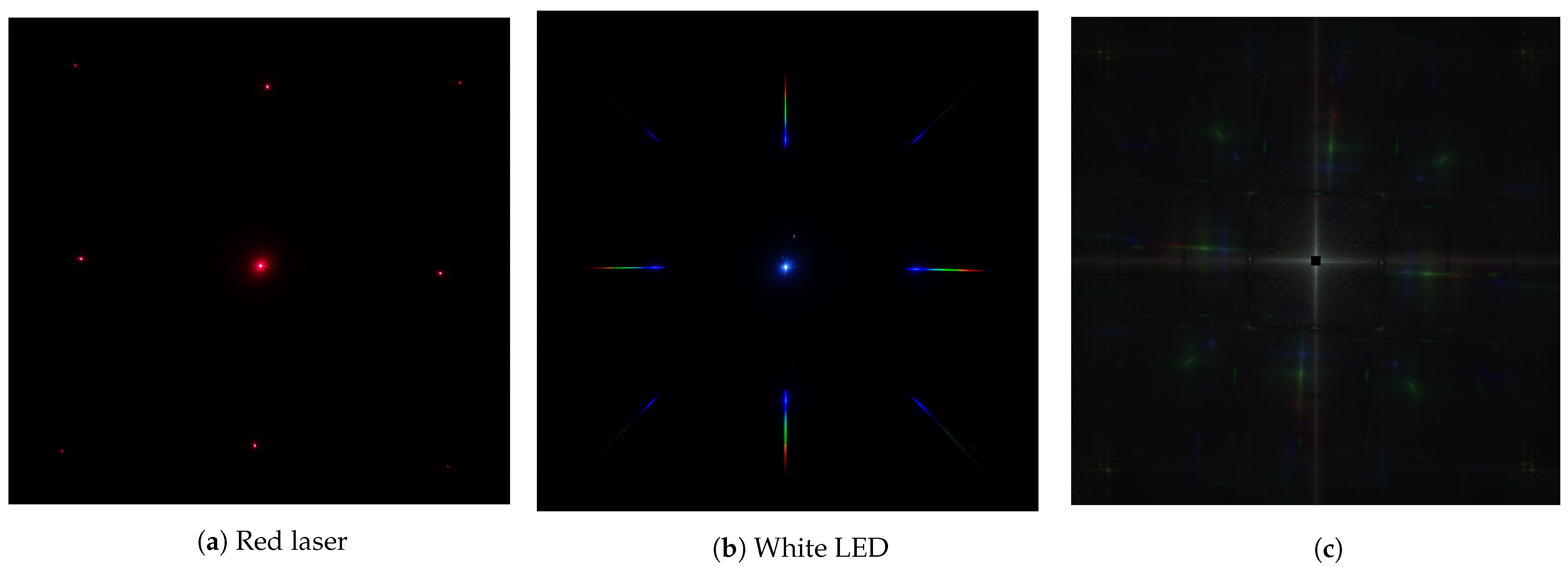
2.1. Diffraction Imaging
2.2. Modeling Diffraction Images
3. Method
3.1. Algorithm 1: Deconvolution
3.2. Algorithm 2: Cepstrum
- Scaling, i.e., multiplication, of the diffraction image affects only the center value of the convolution image;
- Biasing, i.e., addition, the diffraction image leads to a biasing in the convolution image that is nonlinearly relational to the biasing factor;
- Convolution in the diffraction image can be expressed as the sum of two cepstrum images;
- Rotation of the diffraction image results in a rotation of the cepstral image;
- The cepstrum image is invariant to shifts in the diffraction image.
3.2.1. Cepstrum Profile
4. Imaging
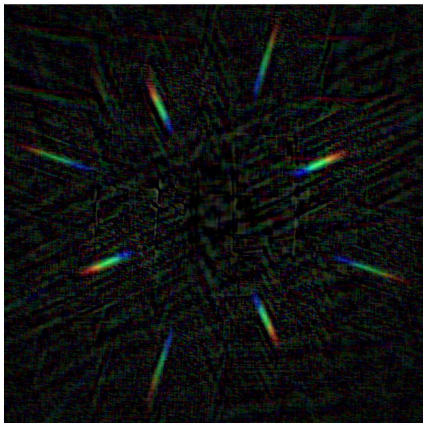
4.1. Diffraction Image
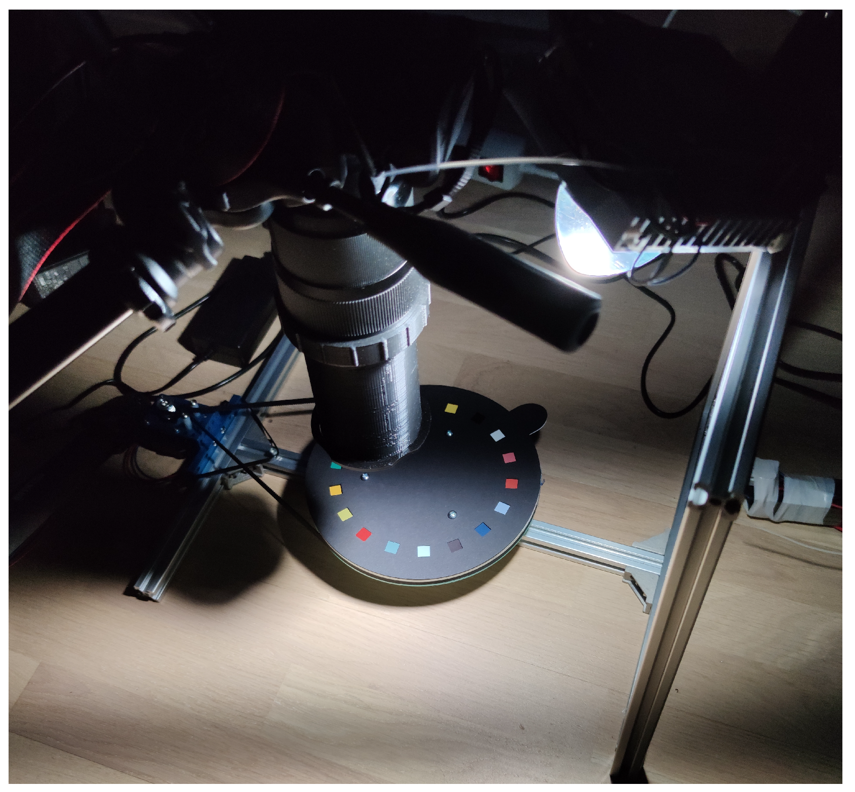
4.2. Imaging Setup
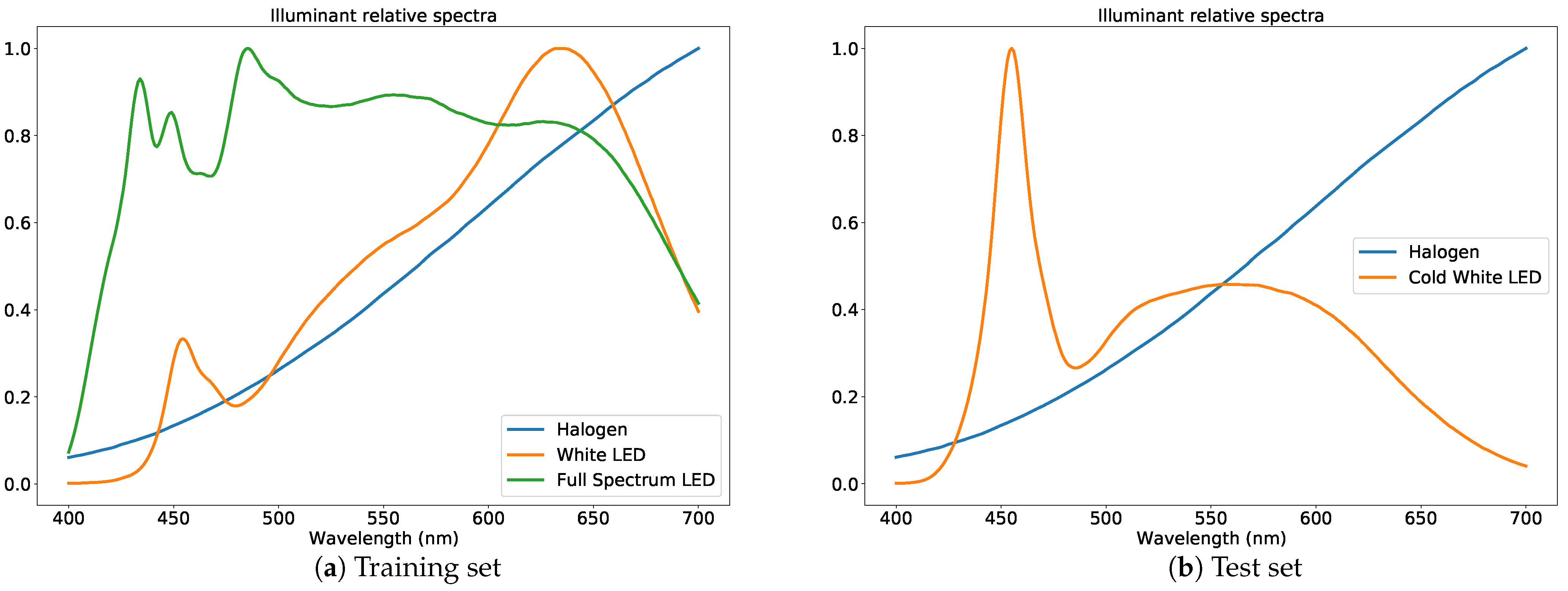
4.3. Data
5. Computational Pipeline
5.1. Calibration
5.2. Deconvolution
5.3. Cepstrum
5.4. Training
5.5. Testing Procedure
6. Results
7. Discussion and Conclusions
Author Contributions
Funding
Conflicts of Interest
References
- Ohno, Y. Spectral color measurement. In Colorimetry: Understanding the CIE System; CIE Central Bureau: Vienna, Austria, 2007; pp. 101–134. [Google Scholar]
- Vane, G.; Goetz, A.F.; Wellman, J.B. Airborne imaging spectrometer: A new tool for remote sensing. IEEE Trans. Geosci. Remote. Sens. 1984, 6, 546–549. [Google Scholar] [CrossRef]
- Goetz, A.F.; Herring, M. The high resolution imaging spectrometer (HIRIS) for EOS. IEEE Trans. Geosci. Remote. Sens. 1989, 27, 136–144. [Google Scholar] [CrossRef]
- Herrala, E.; Okkonen, J.T.; Hyvarinen, T.S.; Aikio, M.; Lammasniemi, J. Imaging spectrometer for process industry applications. Optical Measurements and Sensors for the Process Industries. Int. Soc. Opt. Photon. 1994, 2248, 33–40. [Google Scholar]
- Oke, J.; Cohen, J.; Carr, M.; Cromer, J.; Dingizian, A.; Harris, F.; Labrecque, S.; Lucinio, R.; Schaal, W.; Epps, H.; et al. The Keck low-resolution imaging spectrometer. Publ. Astron. Soc. Pac. 1995, 107, 375. [Google Scholar] [CrossRef] [Green Version]
- Pearlman, J.S.; Barry, P.S.; Segal, C.C.; Shepanski, J.; Beiso, D.; Carman, S.L. Hyperion, a space-based imaging spectrometer. IEEE Trans. Geosci. Remote. Sens. 2003, 41, 1160–1173. [Google Scholar] [CrossRef]
- Cheung, V.; Westland, S.; Li, C.; Hardeberg, J.; Connah, D. Characterization of trichromatic color cameras by using a new multispectral imaging technique. JOSA A 2005, 22, 1231–1240. [Google Scholar] [CrossRef]
- Heikkinen, V.; Lenz, R.; Jetsu, T.; Parkkinen, J.; Hauta-Kasari, M.; Jääskeläinen, T. Evaluation and unification of some methods for estimating reflectance spectra from RGB images. JOSA A 2008, 25, 2444–2458. [Google Scholar] [CrossRef] [PubMed]
- Shimano, N.; Hironaga, M. Recovery of spectral reflectances of imaged objects by the use of features of spectral reflectances. JOSA A 2010, 27, 251–258. [Google Scholar] [CrossRef]
- Peyvandi, S.; Amirshahi, S.H.; Hernandez-Andres, J.; Nieves, J.L.; Romero, J. Generalized inverse-approach model for spectral-signal recovery. IEEE Trans. Image Process. 2012, 22, 501–510. [Google Scholar] [CrossRef]
- Parkkinen, J.P.; Hallikainen, J.; Jaaskelainen, T. Characteristic spectra of Munsell colors. JOSA A 1989, 6, 318–322. [Google Scholar] [CrossRef]
- Imai, F.H.; Berns, R.S.; Tzeng, D.Y. A comparative analysis of spectral reflectance estimated in various spaces using a trichromatic camera system. J. Imaging Sci. Technol. 2000, 44, 280–287. [Google Scholar]
- Attewell, D.; Baddeley, R.J. The distribution of reflectances within the visual environment. Vis. Res. 2007, 47, 548–554. [Google Scholar] [CrossRef] [Green Version]
- Imai, F.H.; Berns, R.S. Spectral estimation using trichromatic digital cameras. In Proceedings of the International Symposium on Multispectral Imaging and Color Reproduction for Digital Archives, Chiba University, Chiba, Japan, 21–22 October 1999; Volume 42, pp. 1–8. [Google Scholar]
- Foster, D.H.; Amano, K. Hyperspectral imaging in color vision research: Tutorial. J. Opt. Soc. Am. A 2019, 36, 606–627. [Google Scholar] [CrossRef]
- Eckhard, J.; Eckhard, T.; Valero, E.M.; Nieves, J.L.; Contreras, E.G. Outdoor scene reflectance measurements using a Bragg-grating-based hyperspectral imager. Appl. Opt. 2015, 54, D15–D24. [Google Scholar] [CrossRef] [Green Version]
- Toivonen, M.E.; Rajani, C.; Klami, A. Snapshot hyperspectral imaging using wide dilation networks. Mach. Vis. Appl. 2021, 32, 1–11. [Google Scholar] [CrossRef]
- Okamoto, T.; Takahashi, A.; Yamaguchi, I. Simultaneous acquisition of spectral and spatial intensity distribution. Appl. Spectrosc. 1993, 47, 1198–1202. [Google Scholar] [CrossRef]
- Johnson, W.R.; Wilson, D.W.; Fink, W.; Humayun, M.S.; Bearman, G.H. Snapshot hyperspectral imaging in ophthalmology. J. Biomed. Opt. 2007, 12, 014036. [Google Scholar] [CrossRef] [PubMed] [Green Version]
- Habel, R.; Kudenov, M.; Wimmer, M. Practical spectral photography. In Computer Graphics Forum; Blackwell Publishing Ltd: Oxford, UK, 2012; Volume 31, pp. 449–458. [Google Scholar]
- Toivonen, M.E.; Klami, A. Practical Camera Sensor Spectral Response and Uncertainty Estimation. J. Imaging 2020, 6, 79. [Google Scholar] [CrossRef] [PubMed]
- Markvart, A.; Liokumovich, L.; Medvedev, I.; Ushakov, N. Continuous Hue-Based Self-Calibration of a Smartphone Spectrometer Applied to Optical Fiber Fabry-Perot Sensor Interrogation. Sensors 2020, 20, 6304. [Google Scholar] [CrossRef]
- Blanchard, P.M.; Greenaway, A.H. Simultaneous multiplane imaging with a distorted diffraction grating. Appl. Opt. 1999, 38, 6692–6699. [Google Scholar] [CrossRef] [PubMed]
- Pan, B.; Wang, Q. Single-camera microscopic stereo digital image correlation using a diffraction grating. Opt. Express 2013, 21, 25056–25068. [Google Scholar] [CrossRef] [PubMed]
- Pan, B.; Yu, L.; Zhang, Q. Review of single-camera stereo-digital image correlation techniques for full-field 3D shape and deformation measurement. Sci. China Technol. Sci. 2018, 61, 2–20. [Google Scholar] [CrossRef] [Green Version]
- Javoršek, D.; Jerman, T.; Rat, B.; Hladnik, A. Assessing the performance of a spectral reflectance estimation method based on a diffraction grating and a spectroradiometer. Color. Technol. 2014, 130, 288–295. [Google Scholar] [CrossRef]
- Rom, R. On the cepstrum of two-dimensional functions (Corresp.). IEEE Trans. Inf. Theory 1975, 21, 214–217. [Google Scholar] [CrossRef]
- Okamoto, T.; Yamaguchi, I. Simultaneous acquisition of spectral image information. Opt. Lett. 1991, 16, 1277–1279. [Google Scholar] [CrossRef]
- Descour, M.; Dereniak, E. Computed-tomography imaging spectrometer: Experimental calibration and reconstruction results. Appl. Opt. 1995, 34, 4817–4826. [Google Scholar] [CrossRef] [PubMed]
- Aikio, M. Hyperspectral prism-grating-prism imaging spectrograph. Ph.D. Thesis, VTT Technical Research Centre of Finland, Espoo, Finland, 16 June 2001. [Google Scholar]
- Jiang, J.; Liu, D.; Gu, J.; Süsstrunk, S. What is the space of spectral sensitivity functions for digital color cameras? In Proceedings of the 2013 IEEE Workshop on Applications of Computer Vision (WACV), Clearwater Beach, FL, USA, 15–17 January 2013; pp. 168–179. [Google Scholar]
- Vrhel, M.J.; Gershon, R.; Iwan, L.S. Measurement and analysis of object reflectance spectra. Color Res. Appl. 1994, 19, 4–9. [Google Scholar] [CrossRef]
- Durmus, D. CIELAB color space boundaries under theoretical spectra and 99 test color samples. Color Res. Appl. 2020, 45, 796–802. [Google Scholar] [CrossRef]
- Hardeberg, J.Y. On the spectral dimensionality of object colors. In Proceedings of the Conference on Colour in Graphics, Imaging, and Vision. Society for Imaging Science and Technology, Poitiers, France, 2–5 April 2002; Volume 2002, pp. 480–485. [Google Scholar]
- Noll, A.M. Cepstrum pitch determination. J. Acoust. Soc. Am. 1967, 41, 293–309. [Google Scholar] [CrossRef]
- Kemerait, R.; Childers, D. Signal detection and extraction by cepstrum techniques. IEEE Trans. Inf. Theory 1972, 18, 745–759. [Google Scholar] [CrossRef]
- Lee, D.J.; Krile, T.F.; Mitra, S. Power cepstrum and spectrum techniques applied to image registration. Appl. Opt. 1988, 27, 1099–1106. [Google Scholar] [CrossRef]
- Gonzalez, R. Robust image registration via cepstral analysis. In Proceedings of the 2011 International Conference on Digital Image Computing: Techniques and Applications, Noosa, QLD, Australia, 6–8 December 2011; pp. 45–50. [Google Scholar]
- Hassab, J.; Boucher, R. Analysis of signal extraction, echo detection and removal by complex cepstrum in presence of distortion and noise. J. Sound Vib. 1975, 40, 321–335. [Google Scholar] [CrossRef]
- Mandava, M. Fast and Robust Cepstral Techniques for Digital Image Registration. Ph.D. Thesis, Texas Tech University, Lubbock, TX, USA, 1992. [Google Scholar]
- Prasad, K.; Unbehauen, R. Analytical expressions of 2-D complex cepstrum. Electron. Lett. 1983, 19, 831–832. [Google Scholar] [CrossRef]
- Van der Walt, S.; Schönberger, J.L.; Nunez-Iglesias, J.; Boulogne, F.; Warner, J.D.; Yager, N.; Gouillart, E.; Yu, T. Scikit-image: Image processing in Python. PeerJ 2014, 2, e453. [Google Scholar] [CrossRef] [PubMed]
- Nogueira, F. Bayesian Optimization: Open Source Constrained Global Optimization Tool for Python. 2014. Available online: https://github.com/fmfn/BayesianOptimization (accessed on 15 January 2021).
- Figuière, H.; Niedermann, H.U. Gphoto. 2021. Available online: https://github.com/gphoto (accessed on 11 January 2021).
- Smith, T.; Guild, J. The CIE colorimetric standards and their use. Trans. Opt. Soc. 1931, 33, 73. [Google Scholar] [CrossRef]
- Behmann, J.; Acebron, K.; Emin, D.; Bennertz, S.; Matsubara, S.; Thomas, S.; Bohnenkamp, D.; Kuska, M.T.; Jussila, J.; Salo, H.; et al. Specim IQ: Evaluation of a new, miniaturized handheld hyperspectral camera and its application for plant phenotyping and disease detection. Sensors 2018, 18, 441. [Google Scholar] [CrossRef] [PubMed] [Green Version]
- Deborah, H.; Richard, N.; Hardeberg, J.Y. A comprehensive evaluation of spectral distance functions and metrics for hyperspectral image processing. IEEE J. Sel. Top. Appl. Earth Obs. Remote. Sens. 2015, 8, 3224–3234. [Google Scholar] [CrossRef]
- Camera Spectral Sensitivity Database. Available online: https://www.gujinwei.org/research/camspec/db.html (accessed on 8 April 2020).
- Spectral Sensitivity Database. Available online: https://nae-lab.org/~rei/research/cs/zhao/database.html (accessed on 8 April 2020).
- Sharma, G.; Wu, W.; Dalal, E.N. The CIEDE2000 Color-Difference Formula: Implementation Notes, Supplementary Test Data, and Mathematical Observations. In Color Research & Application: Endorsed by Inter-Society Color Council, The Colour Group (Great Britain), Canadian Society for Color, Color Science Association of Japan, Dutch Society for the Study of Color, The Swedish Colour Centre Foundation, Colour Society of Australia, Centre Français de la Couleur. Available online: www.interscience.wiley.com (accessed on 28 August 2021).
- Shi, W.; Loy, C.C.; Tang, X. Deep specialized network for illuminant estimation. In European Conference on Computer Vision; Springer: Berlin/Heidelberg, Germany, 11–14 October 2016; pp. 371–387. [Google Scholar]
- Bianco, S.; Cusano, C.; Schettini, R. Single and multiple illuminant estimation using convolutional neural networks. IEEE Trans. Image Process. 2017, 26, 4347–4362. [Google Scholar] [CrossRef] [Green Version]


| Mean of Weighted Canberra Distances | |||||||
|---|---|---|---|---|---|---|---|
| Illuminant | Halogen | Cold White LED | |||||
| Model | Canon M3 | RPI HQ | Samsung S10 | Canon M3 | RPI HQ | Samsung S10 | |
| Deconvolution | Free | 0.0603 | 0.0686 | 0.0359 | 0.1316 | 0.1134 | 0.0586 |
| Non-negative | 0.0552 | 0.0697 | 0.0356 | 0.1274 | 0.1227 | 0.0592 | |
| Cepstrum | Fully connected | 0.1089 | 0.1271 | 0.1364 | 0.2663 | 0.3080 | 0.2045 |
| Simple | 0.1041 | 0.1240 | 0.1272 | 0.2392 | 0.2637 | 0.1995 | |
| Summary Results: Mean of Weighted Canberra Distances | ||||
|---|---|---|---|---|
| Illuminant | Halogen | Cold White LED | ||
| Model | Mean | |||
| Deconvolution | Free | 0.0549 | 0.1010 | 0.0779 |
| Non-negative | 0.0535 | 0.1029 | 0.0781 | |
| Cepstrum | Fully connected | 0.1241 | 0.2591 | 0.1913 |
| Simple | 0.1184 | 0.2339 | 0.1759 | |
| Median of | |||||||
|---|---|---|---|---|---|---|---|
| Illuminant | Halogen | Cold White LED | |||||
| Model | Canon M3 | RPI HQ | Samsung S10 | Canon M3 | RPI HQ | Samsung S10 | |
| Deconvolution | Free | 2.34 | 3.65 | 1.70 | 5.46 | 4.24 | 3.55 |
| Non-negative | 2.40 | 6.94 | 1.63 | 6.20 | 10.99 | 3.38 | |
| Cepstrum | Fully connected | 12.79 | 8.57 | 14.40 | 28.28 | 29.65 | 23.60 |
| Simple | 9.94 | 11.59 | 13.05 | 23.80 | 26.03 | 21.97 | |
| Summary Results: Median of | ||||
|---|---|---|---|---|
| Illuminant | Halogen | Cold White LED | ||
| Model | Median | |||
| Deconvolution | Free | 2.44 | 4.37 | 3.25 |
| Non-negative | 2.72 | 6.85 | 5.08 | |
| Cepstrum | Fully connected | 12.56 | 28.56 | 19.61 |
| Simple | 11.37 | 23.81 | 17.49 | |
Publisher’s Note: MDPI stays neutral with regard to jurisdictional claims in published maps and institutional affiliations. |
© 2021 by the authors. Licensee MDPI, Basel, Switzerland. This article is an open access article distributed under the terms and conditions of the Creative Commons Attribution (CC BY) license (https://creativecommons.org/licenses/by/4.0/).
Share and Cite
Toivonen, M.E.; Talvitie, T.; Rajani, C.; Klami, A. Visible Light Spectrum Extraction from Diffraction Images by Deconvolution and the Cepstrum. J. Imaging 2021, 7, 166. https://doi.org/10.3390/jimaging7090166
Toivonen ME, Talvitie T, Rajani C, Klami A. Visible Light Spectrum Extraction from Diffraction Images by Deconvolution and the Cepstrum. Journal of Imaging. 2021; 7(9):166. https://doi.org/10.3390/jimaging7090166
Chicago/Turabian StyleToivonen, Mikko E., Topi Talvitie, Chang Rajani, and Arto Klami. 2021. "Visible Light Spectrum Extraction from Diffraction Images by Deconvolution and the Cepstrum" Journal of Imaging 7, no. 9: 166. https://doi.org/10.3390/jimaging7090166
APA StyleToivonen, M. E., Talvitie, T., Rajani, C., & Klami, A. (2021). Visible Light Spectrum Extraction from Diffraction Images by Deconvolution and the Cepstrum. Journal of Imaging, 7(9), 166. https://doi.org/10.3390/jimaging7090166