
Multi-Frequency Image Completion via a Biologically-Inspired Sub-Riemannian Model with Frequency and Phase

Abstract
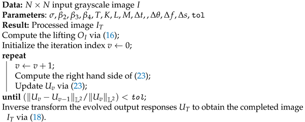
:1. Introduction
2. Model Framework
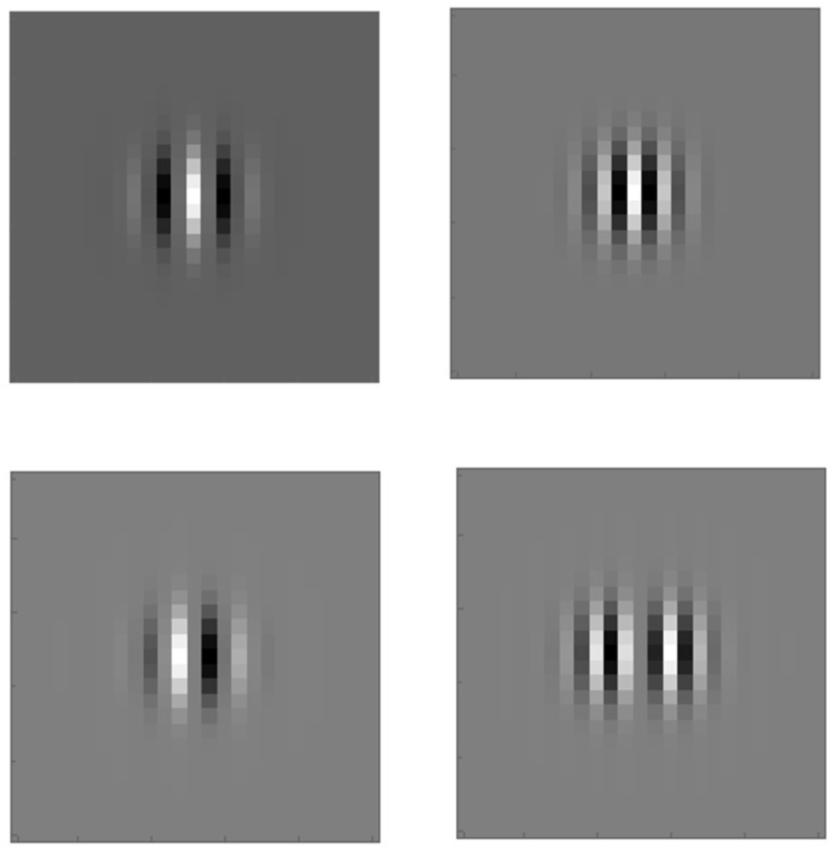
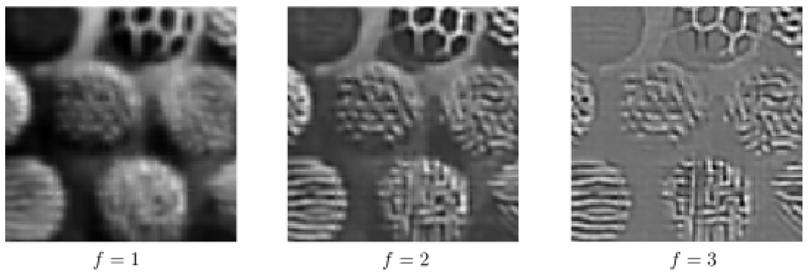
2.1. Feature Value Extraction
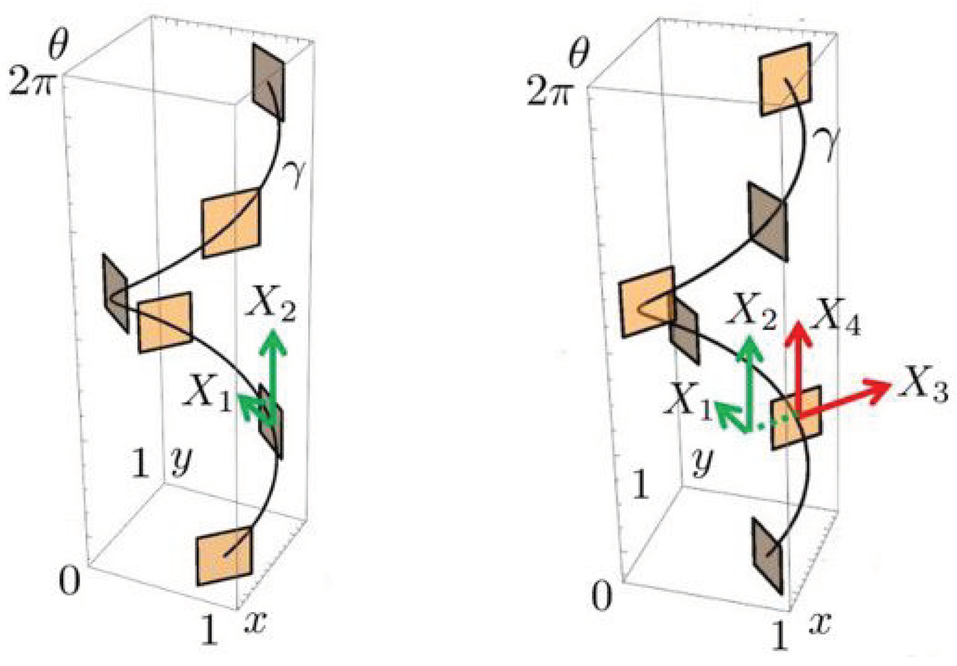
2.2. Horizontal Connectivity
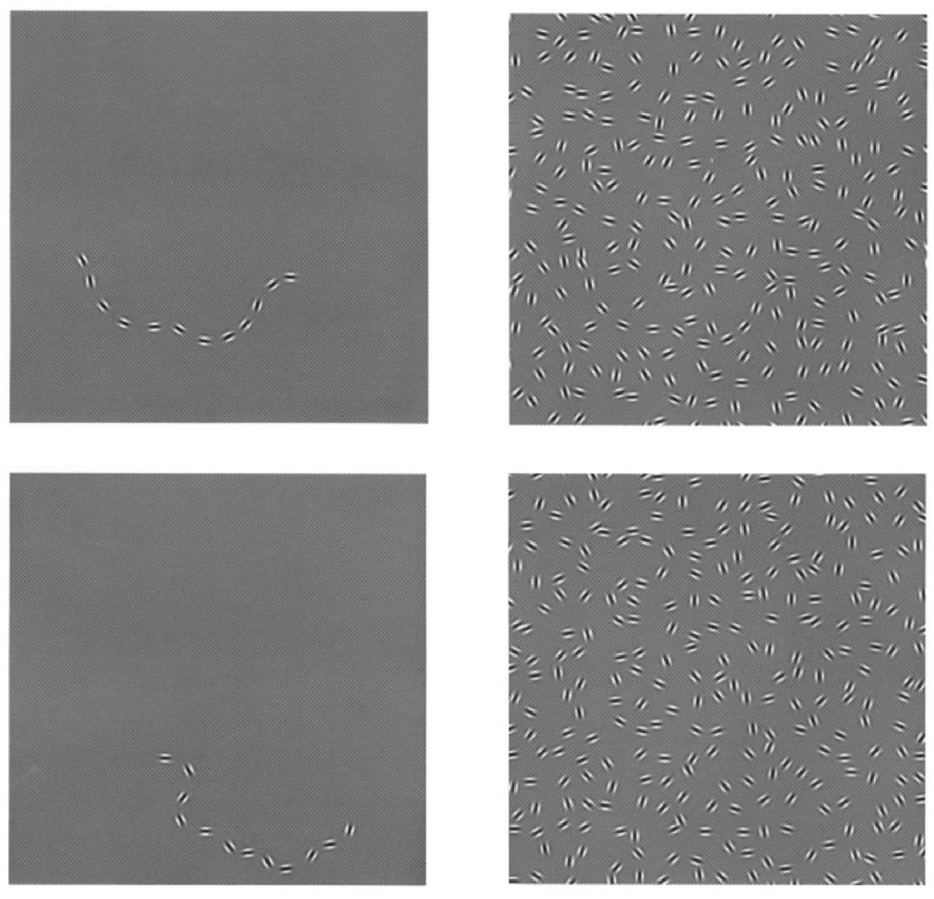
3. Horizontal Integral Curves
4. Sub-Riemannian Diffusion in the Cortical Space
5. Algorithm
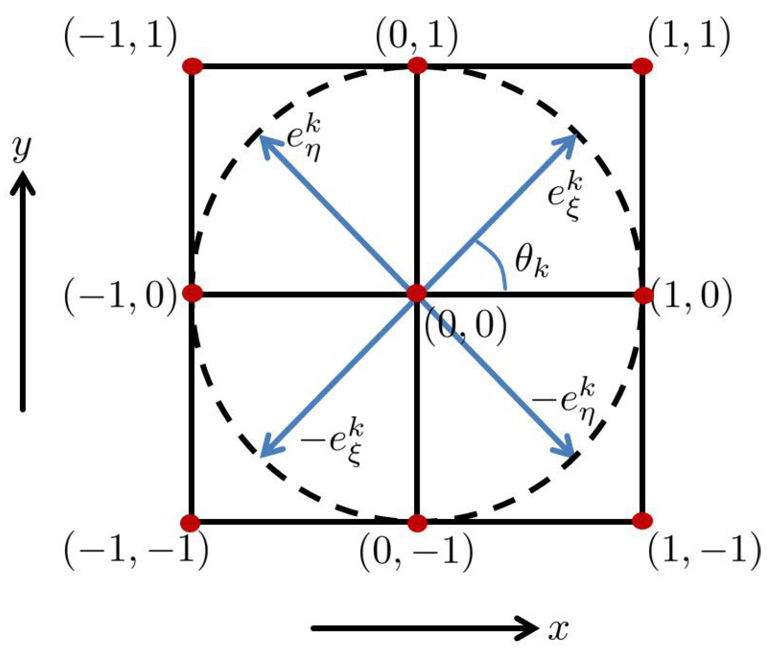
5.1. Discretization of the Output Responses
5.2. Explicit Scheme with Finite Differences
5.3. Pseudocode of the Algorithm
| Algorithm 1: Completion algorithm pseudocode. |
 |
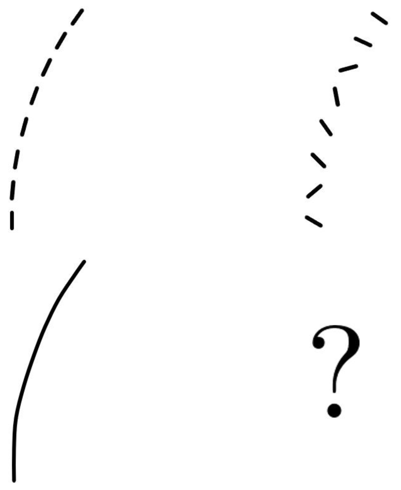
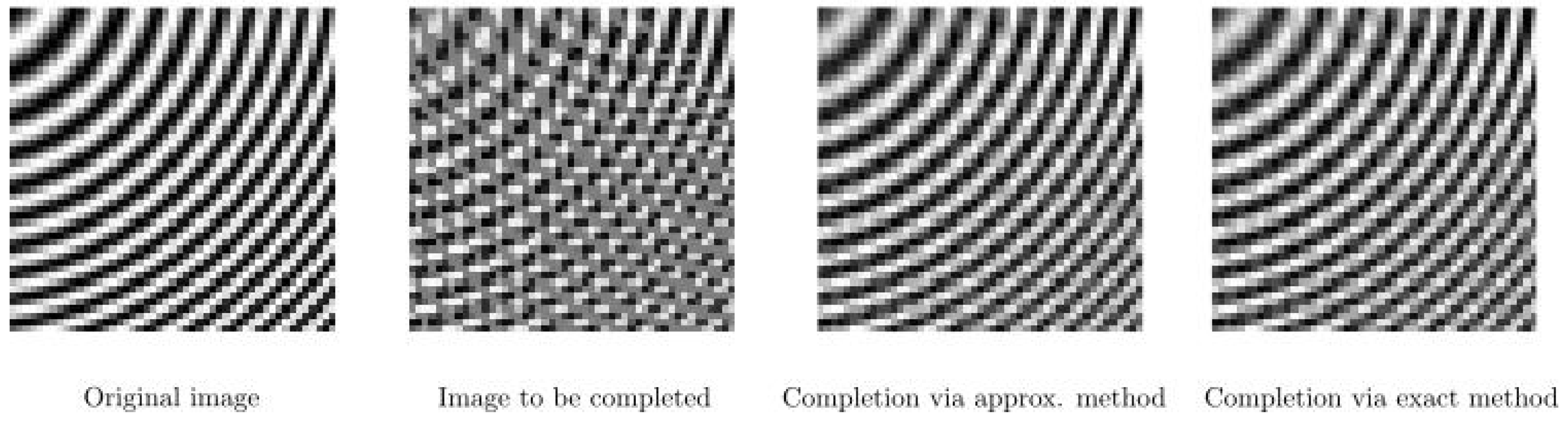
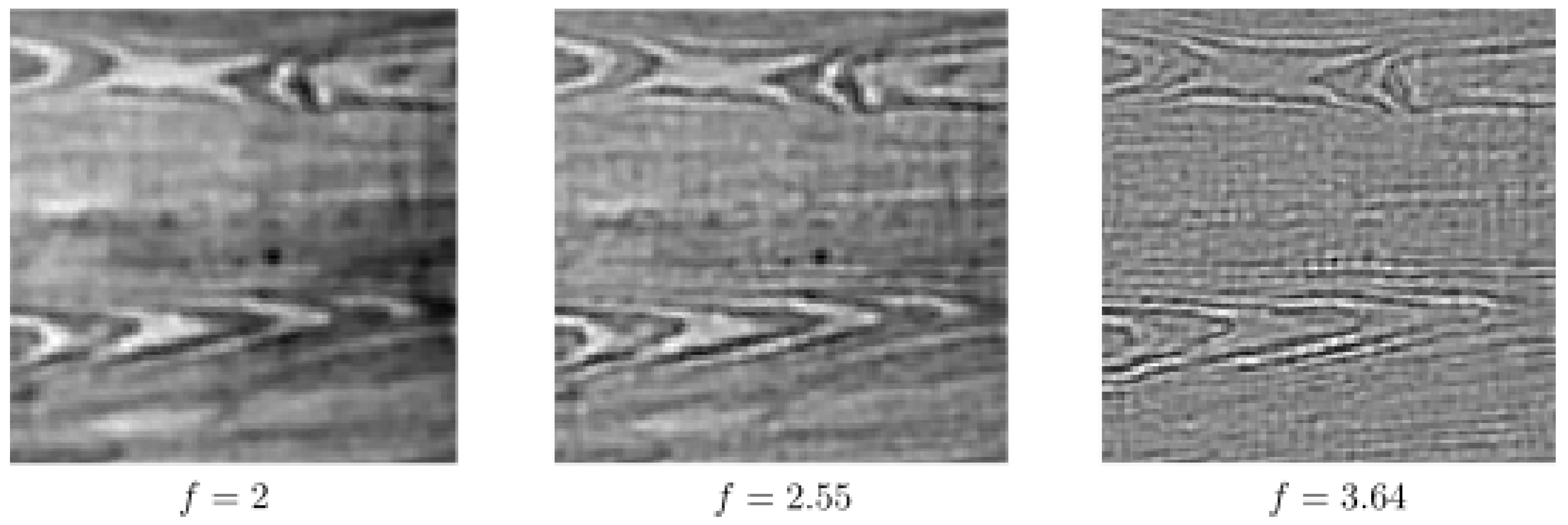
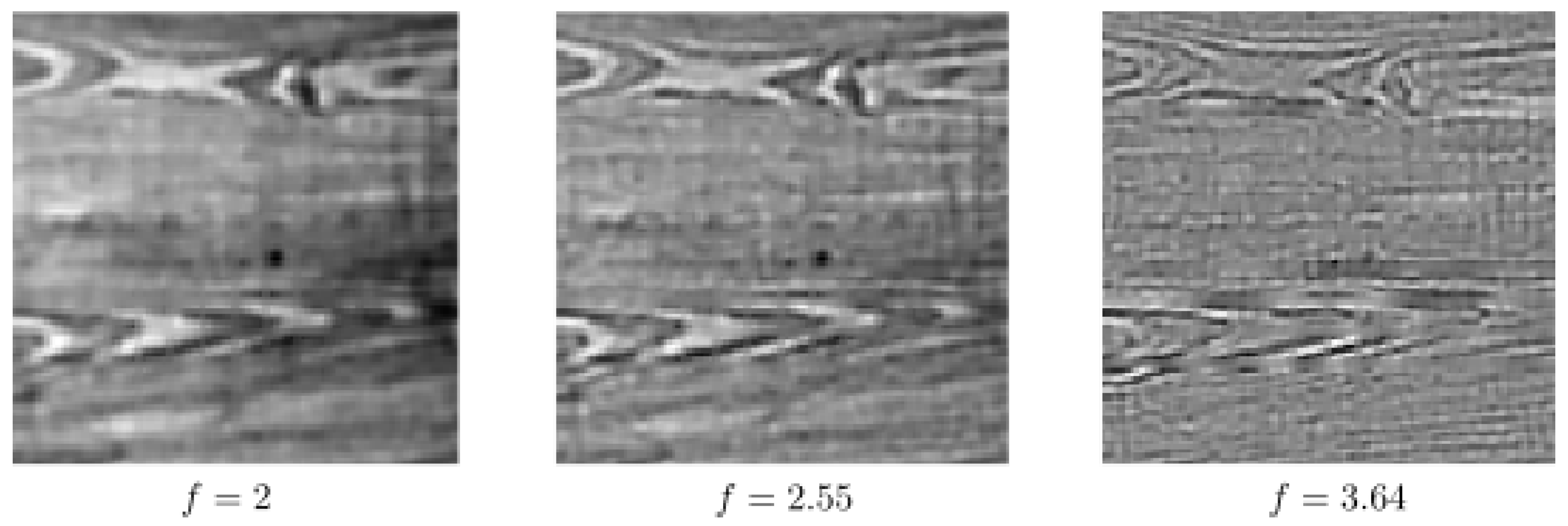
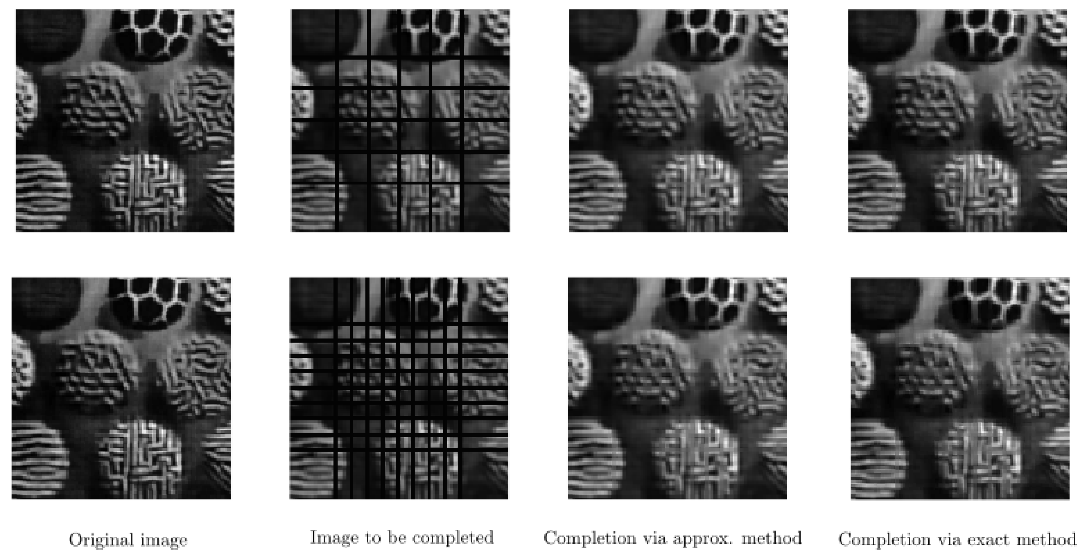
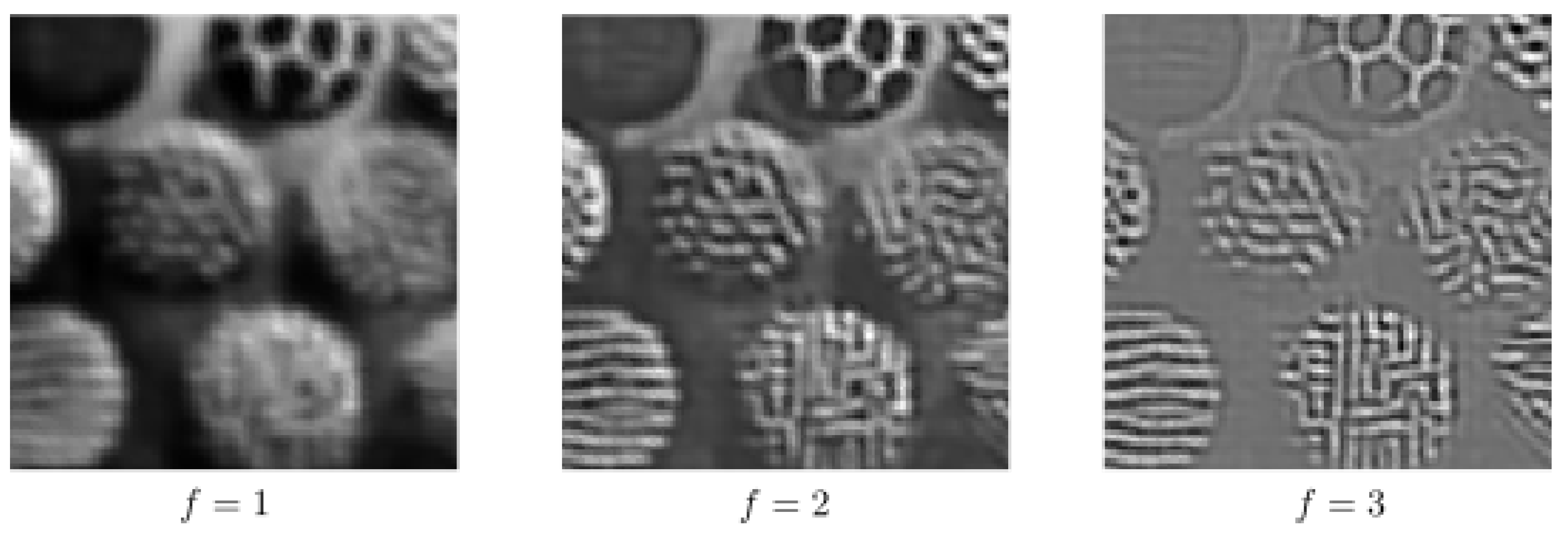
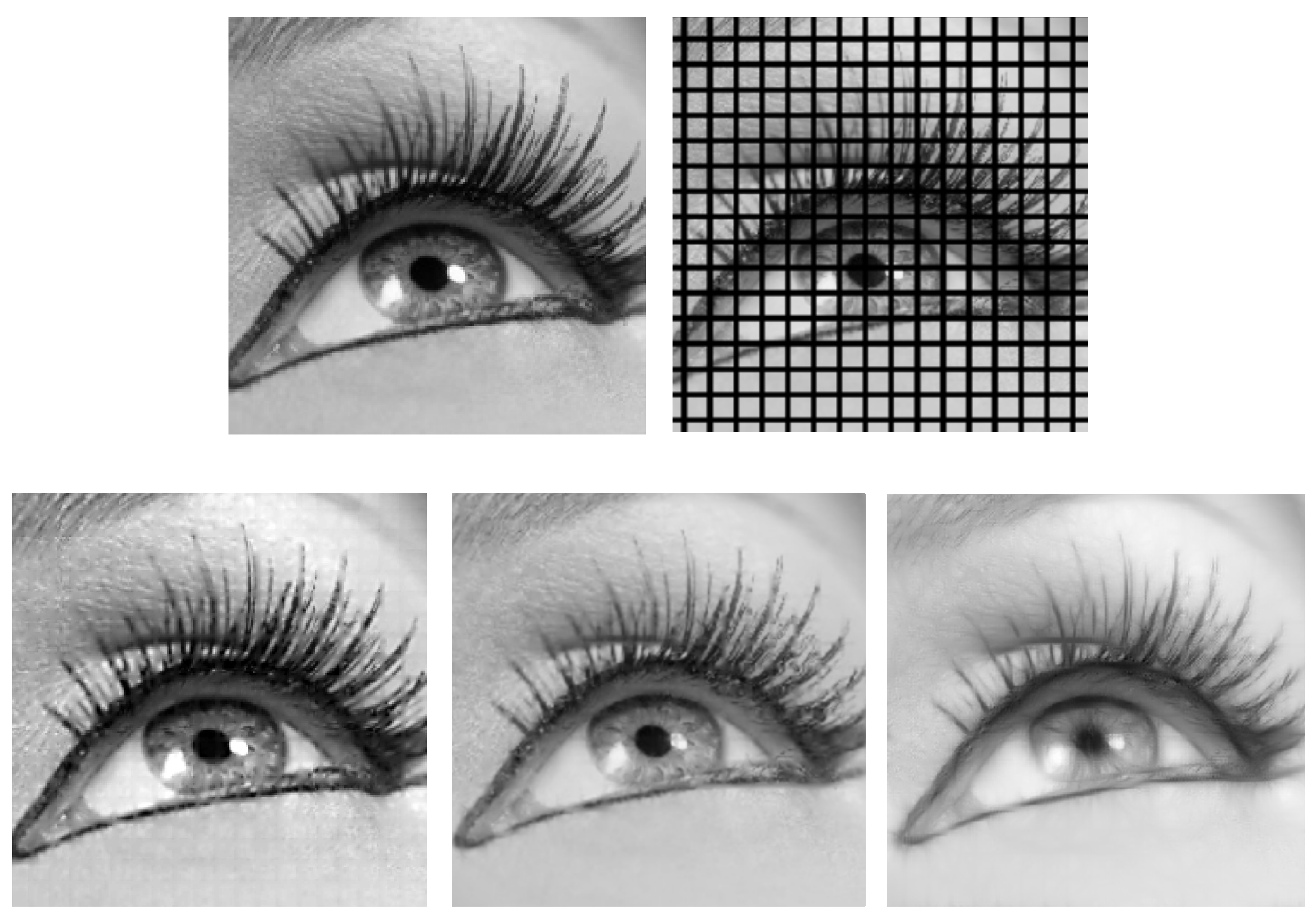
6. Numerical Experiments
7. Conclusions
Funding
Institutional Review Board Statement
Informed Consent Statement
Data Availability Statement
Acknowledgments
Conflicts of Interest
References
- Husserl, E.; Holenstein, E. Logische Untersuchungen. Springer Netherlands: The Hague, The Netherlands, 1975. [Google Scholar]
- Husserl, E.; Claesges, U. Ding und Raum: Vorlesungen 1907; Springer Netherlands: The Hague, The Netherlands, 1973. [Google Scholar]
- Husserl, E.; Schumann, K. Ideen zu einer reinen Phänomenologie und phänomenologischen Philosophie; Springer Netherlands: The Hague, The Netherlands, 1976. [Google Scholar]
- Wertheimer, M. Laws of Organization in Perceptual Forms. In A Source Book of Gestalt Psychology; Ellis, W.D., Ed.; Trubner & Company: Kegan Paul, Trench, 1938; pp. 71–88. [Google Scholar] [CrossRef]
- Köhler, W. Gestalt Psychology: An Introduction to New Concepts in Modern Psychology; Liveright: New York, NY, USA, 1970. [Google Scholar]
- Koffka, K. Principles of Gestalt Psychology; Routledge: Abingdon, UK, 2013; Volume 44. [Google Scholar]
- Field, D.J.; Hayes, A.; Hess, R.F. Contour integration by the human visual system: Evidence for a local “association field”. Vis. Res. 1993, 33, 173–193. [Google Scholar] [CrossRef]
- Kanizsa, G. Organization in Vision: Essays on Gestalt Perception; Praeger Publishers: Westport, CT, USA, 1979. [Google Scholar]
- Kanizsa, G. Grammatica del Vedere: Saggi su Percezione e Gestalt; Il Mulino: Bologna, Italy, 1980. [Google Scholar]
- Hubel, D.H.; Wiesel, T.N. Receptive fields of single neurones in the cat’s striate cortex. J. Physiol. 1959, 148, 574. [Google Scholar] [CrossRef] [PubMed]
- Hubel, D.H.; Wiesel, T.N. Receptive fields, binocular interaction and functional architecture in the cat’s visual cortex. J. Physiol. 1962, 160, 106. [Google Scholar] [CrossRef] [PubMed]
- Hubel, D.H.; Wiesel, T.N. Shape and arrangement of columns in cat’s striate cortex. J. Physiol. 1963, 165, 559. [Google Scholar] [CrossRef] [PubMed] [Green Version]
- Hubel, D.H.; Wiesel, T.N. Uniformity of monkey striate cortex: A parallel relationship between field size, scatter, and magnification factor. J. Comp. Neurol. 1974, 158, 295–305. [Google Scholar] [CrossRef]
- Hubel, D.H.; Wiesel, T.N. Ferrier lecture: Functional architecture of macaque monkey visual cortex. Proc. R. Soc. Lond. Biol. Sci. 1977, 198, 1–59. [Google Scholar]
- Maffei, L.; Fiorentini, A. Spatial frequency rows in the striate visual cortex. Vis. Res. 1977, 17, 257–264. [Google Scholar] [CrossRef]
- Hübener, M.; Shoham, D.; Grinvald, A.; Bonhoeffer, T. Spatial relationships among three columnar systems in cat area 17. J. Neurosci. 1997, 17, 9270–9284. [Google Scholar] [CrossRef] [Green Version]
- Issa, N.P.; Trepel, C.; Stryker, M.P. Spatial frequency maps in cat visual cortex. J. Neurosci. 2000, 20, 8504–8514. [Google Scholar] [CrossRef] [Green Version]
- Issa, N.P.; Rosenberg, A.; Husson, T.R. Models and measurements of functional maps in V1. J. Neurophysiol. 2008, 99, 2745–2754. [Google Scholar] [CrossRef] [Green Version]
- Sirovich, L.; Uglesich, R. The organization of orientation and spatial frequency in primary visual cortex. Proc. Natl. Acad. Sci. USA 2004, 101, 16941–16946. [Google Scholar] [CrossRef] [PubMed] [Green Version]
- Tani, T.; Ribot, J.; O’Hashi, K.; Tanaka, S. Parallel development of orientation maps and spatial frequency selectivity in cat visual cortex. Eur. J. Neurosci. 2012, 35, 44–55. [Google Scholar] [CrossRef] [PubMed]
- Ribot, J.; Aushana, Y.; Bui-Quoc, E.; Milleret, C. Organization and origin of spatial frequency maps in cat visual cortex. J. Neurosci. 2013, 33, 13326–13343. [Google Scholar] [CrossRef] [Green Version]
- Ribot, J.; Romagnoni, A.; Milleret, C.; Bennequin, D.; Touboul, J. Pinwheel-dipole configuration in cat early visual cortex. NeuroImage 2016, 128, 63–73. [Google Scholar] [CrossRef] [PubMed]
- De Valois, K.; Tootell, R.B. Spatial-frequency-specific inhibition in cat striate cortex cells. J. Physiol. 1983, 336, 359–376. [Google Scholar] [CrossRef] [Green Version]
- Pollen, D.A.; Gaska, J.P.; Jacobson, L.D. Responses of simple and complex cells to compound sine-wave gratings. Vis. Res. 1988, 28, 25–39. [Google Scholar] [CrossRef]
- Levitt, J.B.; Sanchez, R.M.; Smith, E.L.; Movshon, J.A. Spatio-temporal interactions and the spatial phase preferences of visual neurons. Exp. Brain Res. 1990, 80, 441–445. [Google Scholar] [CrossRef]
- Mechler, F.; Reich, D.S.; Victor, J.D. Detection and discrimination of relative spatial phase by V1 neurons. J. Neurosci. 2002, 22, 6129–6157. [Google Scholar] [CrossRef] [Green Version]
- Blakemore, C.T.; Campbell, F.W. On the existence of neurones in the human visual system selectively sensitive to the orientation and size of retinal images. J. Physiol. 1969, 203, 237. [Google Scholar] [CrossRef]
- Shatz, C.J.; Stryker, M.P. Ocular dominance in layer iv of the cat’s visual cortex and the effects of monocular deprivation. J. Physiol. 1978, 281, 267–283. [Google Scholar] [CrossRef] [Green Version]
- LeVay, S.; Stryker, M.P.; Shatz, C.J. Ocular dominance columns and their development in layer iv of the cat’s visual cortex: A quantitative study. J. Comp. Neurol. 1978, 179, 223–244. [Google Scholar] [CrossRef]
- Hoffman, W.C. Higher visual perception as prolongation of the basic lie transformation group. Math. Biosci. 1970, 6, 437–471. [Google Scholar] [CrossRef]
- Hoffman, W.C. The visual cortex is a contact bundle. Appl. Math. Comput. 1989, 32, 137–167. [Google Scholar] [CrossRef]
- Petitot, J.; Tondut, Y. Vers une neurogéométrie. fibrations corticales, structures de contact et contours subjectifs modaux. Math. Sci. Hum. 1999, 145, 5–101. [Google Scholar] [CrossRef] [Green Version]
- Citti, G.; Sarti, A. A cortical based model of perceptual completion in the roto-translation space. J. Math. Imaging Vis. 2006, 24, 307–326. [Google Scholar] [CrossRef]
- Sarti, A.; Citti, G.; Petitot, J. The symplectic structure of the primary visual cortex. Biol. Cybern. 2008, 98, 33–48. [Google Scholar] [CrossRef]
- Barbieri, D.; Citti, G.; Cocci, G.; Sarti, A. A cortical-inspired geometry for contour perception and motion integration. J. Math. Imaging Vis. 2014, 49, 511–529. [Google Scholar] [CrossRef] [Green Version]
- Cocci, G.; Barbieri, D.; Citti, G.; Sarti, A. Cortical spatiotemporal dimensionality reduction for visual grouping. Neural Comput. 2015, 27, 1252–1293. [Google Scholar] [CrossRef] [PubMed]
- Franceschiello, B.; Mashtakov, A.; Citti, G.; Sarti, A. Geometrical optical illusion via sub-Riemannian geodesics in the roto-translation group. Differ. Geom. Its Appl. 2019, 65, 55–77. [Google Scholar] [CrossRef] [Green Version]
- Franceschiello, B.; Sarti, A.; Citti, G. A neuromathematical model for geometrical optical illusions. J. Math. Imaging Vis. 2018, 60, 94–108. [Google Scholar] [CrossRef] [Green Version]
- Bertalmío, M.; Calatroni, L.; Franceschi, V.; Franceschiello, B.; Villa, A.G.; Prandi, D. Visual illusions via neural dynamics: Wilson–Cowan-type models and the efficient representation principle. J. Neurophysiol. 2020, 123, 1606–1618. [Google Scholar] [CrossRef] [Green Version]
- Bertalmio, M.; Calatroni, L.; Franceschi, V.; Franceschiello, B.; Prandi, D. Cortical-inspired Wilson-Cowan-type equations for orientation-dependent contrast perception modelling. J. Math. Imaging Vis. 2021, 63, 263–281. [Google Scholar] [CrossRef]
- Baspinar, E.; Calatroni, L.; Franceschi, V.; Prandi, D. A cortical-inspired sub-Riemannian model for Poggendorff-type visual illusions. J. Imaging 2021, 7, 41. [Google Scholar] [CrossRef]
- Baspinar, E.; Citti, G.; Sarti, A. A geometric model of multi-scale orientation preference maps via Gabor functions. J. Math. Imaging Vis. 2018, 60, 900–912. [Google Scholar] [CrossRef] [Green Version]
- Duits, R.; Franken, E. Left-invariant parabolic evolutions on SE(2) and contour enhancement via invertible orientation scores part I: Linear left-invariant diffusion equations on SE(2). Q. Appl. Math. 2010, 68, 255–292. [Google Scholar] [CrossRef] [Green Version]
- Duits, R.; Franken, E. Left-invariant parabolic evolutions on se(2) and contour enhancement via invertible orientation scores part ii: Nonlinear left-invariant diffusions on invertible orientation scores. Q. Appl. Math. 2010, 68, 293–331. [Google Scholar] [CrossRef] [Green Version]
- Boscain, U.; Duplaix, J.; Gauthier, J.P.; Rossi, F. Anthropomorphic image reconstruction via hypoelliptic diffusion. SIAM J. Control Optim. 2012, 50, 1309–1336. [Google Scholar] [CrossRef]
- Duits, R.; Führ, H.; Janssen, B.; Bruurmijn, M.; Florack, L.; van Assen, H. Evolution equations on Gabor transforms and their applications. Appl. Comput. Harmon. Anal. 2013, 35, 483–526. [Google Scholar] [CrossRef]
- Boscain, U.; Gauthier, J.P.; Prandi, D.; Remizov, A. Image reconstruction via non-isotropic diffusion in Dubins/Reed-Shepp-like control systems. In Proceedings of the 53rd IEEE Conference on Decision and Control, Los Angeles, CA, USA, 15–17 December 2014; IEEE: Piscataway, NJ, USA, 2014; pp. 4278–4283. [Google Scholar]
- Boscain, U.; Chertovskih, R.A.; Gauthier, J.P.; Remizov, A.O. Hypoelliptic diffusion and human vision: A semidiscrete new twist. SIAM J. Imaging Sci. 2014, 7, 669–695. [Google Scholar] [CrossRef]
- Sharma, U.; Duits, R. Left-invariant evolutions of wavelet transforms on the similitude group. Appl. Comput. Harmon. Anal. 2015, 39, 110–137. [Google Scholar] [CrossRef]
- Citti, G.; Franceschiello, B.; Sanguinetti, G.; Sarti, A. Sub-Riemannian mean curvature flow for image processing. SIAM J. Imaging Sci. 2016, 9, 212–237. [Google Scholar] [CrossRef] [Green Version]
- Prandi, D.; Gauthier, J.-P. A Semidiscrete Version of the Citti-Petitot-Sarti Model as a Plausible Model for Anthropomorphic Image Reconstruction and Pattern Recognition; Springer Briefs in Mathematics; Springer: Cham, Switzerland, 2018. [Google Scholar] [CrossRef] [Green Version]
- ter Haar Romeny, B.M.; Bekkers, E.J.; Zhang, J.; Abbasi-Sureshjani, S.; Huang, F.; Duits, R.; Dashtbozorg, B.; Berendschot, T.T.J.M.; Smit-Ockeloen, I.; Eppenhof, K.A.J.; et al. Brain-inspired algorithms for retinal image analysis. Mach. Vis. Appl. 2016, 27, 1117–1135. [Google Scholar] [CrossRef] [Green Version]
- Bekkers, E.; Duits, R.; Berendschot, T.; Romeny, B.H. A multi-orientation analysis approach to retinal vessel tracking. J. Math. Imaging Vis. 2014, 49, 583–610. [Google Scholar] [CrossRef] [Green Version]
- Bosking, W.H.; Zhang, Y.; Schofield, B.; Fitzpatrick, D. Orientation selectivity and the arrangement of horizontal connections in tree shrew striate cortex. J. Neurosci. 1997, 17, 2112–2127. [Google Scholar] [CrossRef] [PubMed]
- Baspinar, E.; Sarti, A.; Citti, G. A sub-Riemannian model of the visual cortex with frequency and phase. J. Math. Neurosci. 2020, 10, 1–31. [Google Scholar] [CrossRef] [PubMed]
- Baspinar, E. Minimal Surfaces in Sub-Riemannian Structures and Functional Geometry of the Visual Cortex. Dissertation Thesis, Alma Mater Studiorum Università di Bologna, Bologna, Italy, 2018. [Google Scholar]
- Daugman, J.G. Uncertainty relation for resolution in space, spatial frequency, and orientation optimized by two-dimensional visual cortical filters. JOSA A 1985, 2, 1160–1169. [Google Scholar] [CrossRef]
- Bekkers, E.J.; Lafarge, M.W.; Veta, M.; Eppenhof, K.A.J.; Pluim, J.P.W.; Duits, R. Roto-translation covariant convolutional networks for medical image analysis. In International Conference on Medical Image Computing and Computer-Assisted Intervention; Springer: Berlin/Heidelberg, Germany, 2018; pp. 440–448. [Google Scholar]
- Duits, R.; Duits, M.; van Almsick, M.; Romeny, B.H. Invertible orientation scores as an application of generalized wavelet theory. Pattern Recognit. Image Anal. 2007, 17, 42–75. [Google Scholar] [CrossRef] [Green Version]
- Koenderink, J.J.; van Doorn, A.J. Representation of local geometry in the visual system. Biol. Cybern. 1987, 55, 367–375. [Google Scholar] [CrossRef] [PubMed]
- Lindeberg, T. A computational theory of visual receptive fields. Biol. Cybern. 2013, 107, 589–635. [Google Scholar] [CrossRef]
- Hörmander, L. Hypoelliptic second order differential equations. Acta Math. 1967, 119, 147–171. [Google Scholar] [CrossRef]
- Rashevskii, P.K. Any two points of a totally nonholonomic space may be connected by an admissible line. Uch. Zap. Ped. Inst. Liebknechta Ser. Phys. Math. 1938, 2, 83–94. [Google Scholar]
- Chow, W.-L. Über systeme von linearen partiellen differentialgleichungen erster ordnung. Math. Ann. 1940, 117, 98–105. [Google Scholar] [CrossRef]
- Agrachev, A.; Barilari, D.; Boscain, U. A Comprehensive Introduction to Sub-Riemannian Geometry; Cambridge University Press: Cambridge, UK, 2019; Volume 181. [Google Scholar]
- Unser, M. Splines: A perfect fit for signal and image processing. IEEE Signal Process. Mag. 1999, 16, 22–38. [Google Scholar] [CrossRef] [Green Version]
- Franken, E.M. Enhancement of Crossing Elongated Structures in Images; Eindhoven University of Technology: Eindhoven, The Netherlands, 2008. [Google Scholar]
- Kimmel, R.; Malladi, R.; Sochen, N. Images as embedded maps and minimal surfaces: Movies, color, texture, and volumetric medical images. Int. J. Comput. Vis. 2000, 39, 111–129. [Google Scholar] [CrossRef]
- Boscain, U.V.; Chertovskih, R.; Gauthier, J.P.; Prandi, D.; Remizov, A. Highly corrupted image inpainting through hypoelliptic diffusion. J. Math. Imaging Vis. 2018, 60, 1231–1245. [Google Scholar] [CrossRef] [Green Version]
- Duits, R.; Almsick, M.V. The explicit solutions of linear left-invariant second order stochastic evolution equations on the 2d euclidean motion group. Q. Appl. Math. 2008, 66, 27–67. [Google Scholar] [CrossRef] [Green Version]
- Zhang, J.; Duits, R.; Sanguinetti, G.; ter Haar Romeny, B.M. Numerical approaches for linear left-invariant diffusions on se (2), their comparison to exact solutions, and their applications in retinal imaging. Numer. Math. Theory Methods Appl. 2016, 9, 1–50. [Google Scholar] [CrossRef] [Green Version]


Publisher’s Note: MDPI stays neutral with regard to jurisdictional claims in published maps and institutional affiliations. |
© 2021 by the author. Licensee MDPI, Basel, Switzerland. This article is an open access article distributed under the terms and conditions of the Creative Commons Attribution (CC BY) license (https://creativecommons.org/licenses/by/4.0/).
Share and Cite
Baspinar, E. Multi-Frequency Image Completion via a Biologically-Inspired Sub-Riemannian Model with Frequency and Phase. J. Imaging 2021, 7, 271. https://doi.org/10.3390/jimaging7120271
Baspinar E. Multi-Frequency Image Completion via a Biologically-Inspired Sub-Riemannian Model with Frequency and Phase. Journal of Imaging. 2021; 7(12):271. https://doi.org/10.3390/jimaging7120271
Chicago/Turabian StyleBaspinar, Emre. 2021. "Multi-Frequency Image Completion via a Biologically-Inspired Sub-Riemannian Model with Frequency and Phase" Journal of Imaging 7, no. 12: 271. https://doi.org/10.3390/jimaging7120271
APA StyleBaspinar, E. (2021). Multi-Frequency Image Completion via a Biologically-Inspired Sub-Riemannian Model with Frequency and Phase. Journal of Imaging, 7(12), 271. https://doi.org/10.3390/jimaging7120271