
Brain Tumor Segmentation Based on Deep Learning’s Feature Representation

Abstract
:1. Introduction
2. Related Work
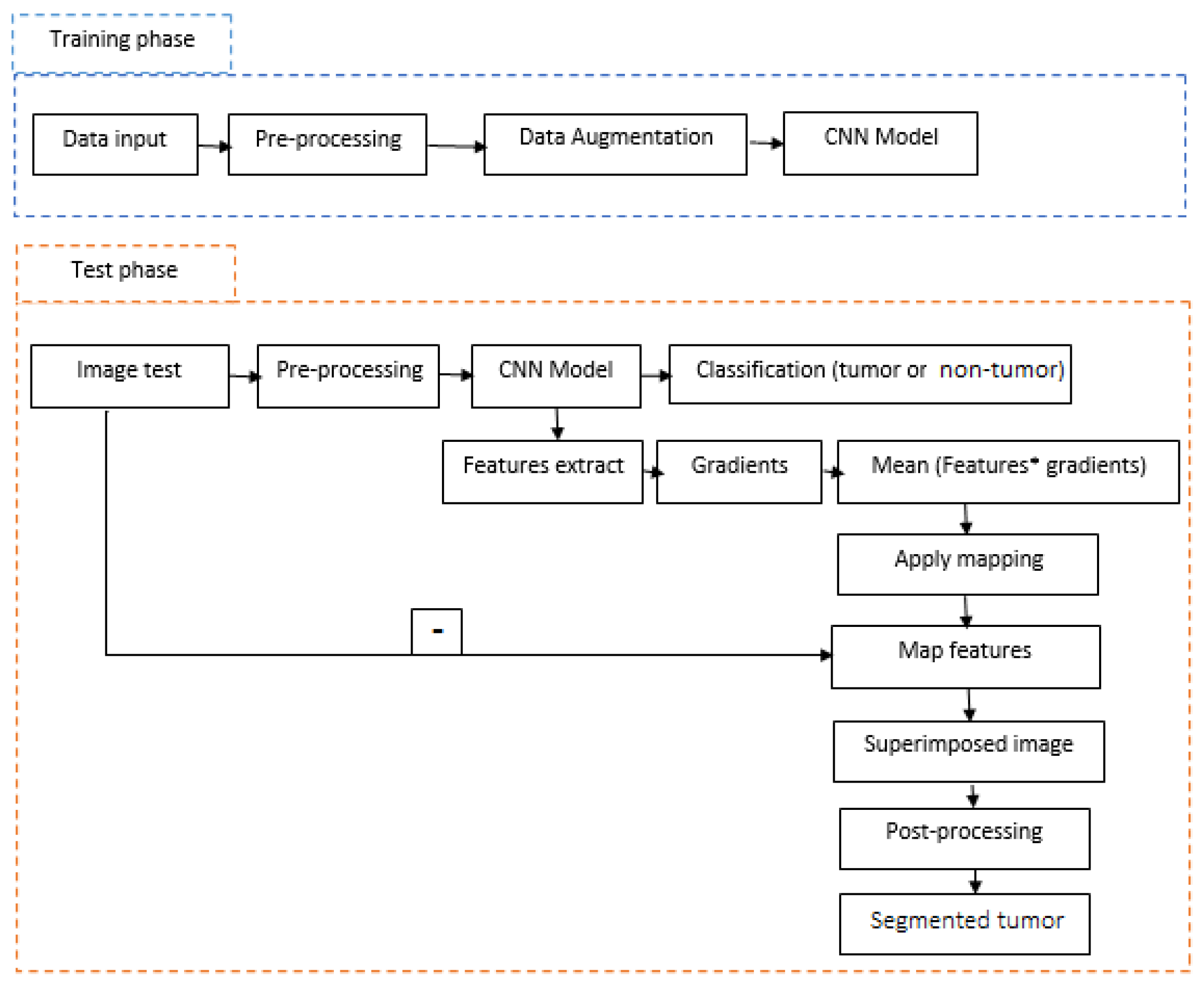
3. Proposed Method
3.1. Pre-Processing
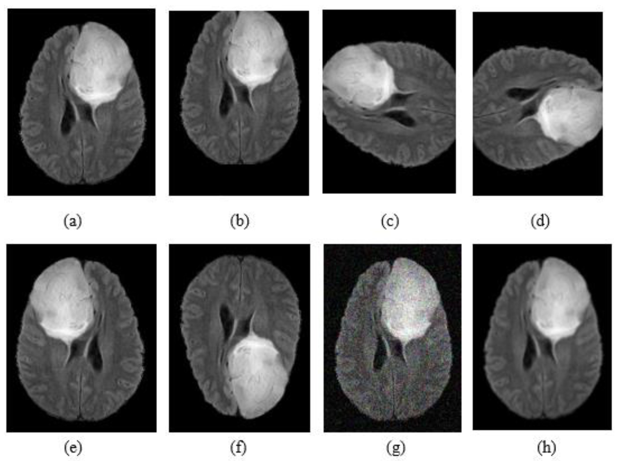
3.2. Data Augmentation
3.3. Convolution Neural Networks
3.3.1. Tumor Classification (Tumor or Not Tumor)
3.3.2. Tumor Segmentation
3.4. Post-Processing
4. Experimental Setup
4.1. Dataset
4.2. Implementation Details
4.3. Performance Evaluation
- Precision: It is the percentage of results that are relevant and is defined as:
- Recall: The percentage of total relevant results correctly classified by the proposed algorithm which is defined as:
- Accuracy: Formally, accuracy has the following definition:
- The DSC represents the overlapping of predicted segmentation with the manually segmented output label and is computed as:
5. Results and Discussion
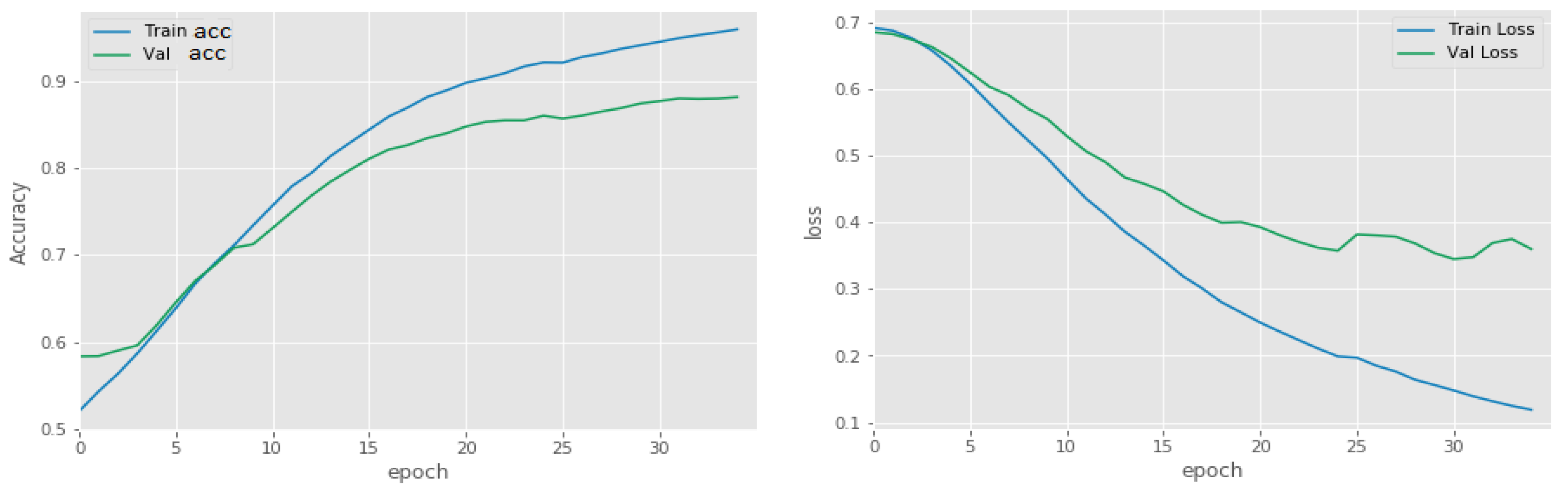
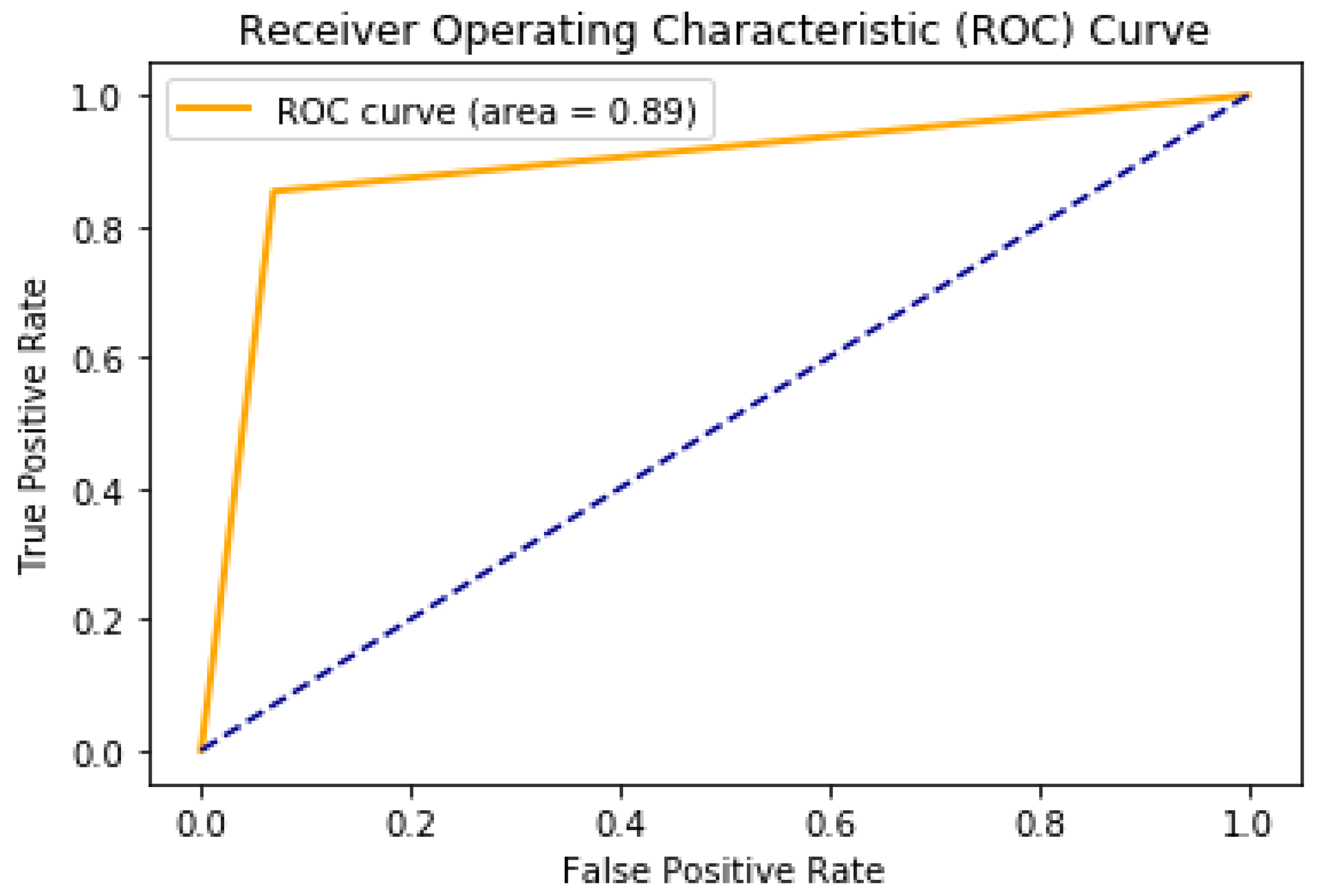
5.1. Binary Classification of Tumor or Non-Tumor
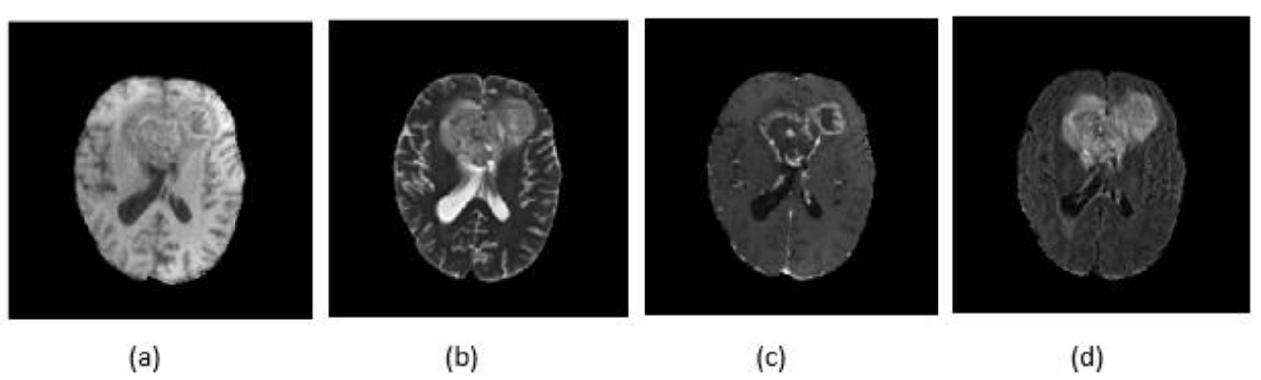
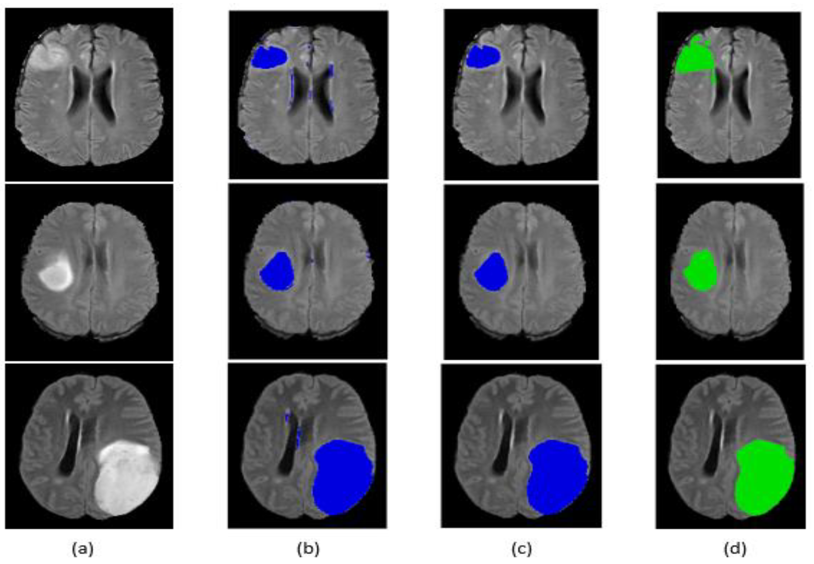
5.2. Tumor Segmentation
6. Conclusions
Author Contributions
Funding
Institutional Review Board Statement
Informed Consent Statement
Data Availability Statement
Conflicts of Interest
References
- Laszlo, L.; Lefkovits, S.; Vaida, M.F. Brain tumor segmentation based on random forest. Mem. Sci. Sect. Rom. Acad. 2016, 1, 83–93. [Google Scholar]
- Szabó, Z.; Kapa, Z.; Lefkovits, L.; Gyor, A.; Szilagy, S.M.; Szilagy, L. Automatic segmentation of low-grade brain tumor using a random forest classifier and Gabor features. In Proceedings of the 14th International Conference on Natural Computation, Fuzzy Systems and Knowledge Discove, Huangshan, China, 28–30 July 2018; pp. 1106–1113. [Google Scholar]
- Zhang, J.; Ma, K.K.; Er, M.H.; Chong, V. Tumor segmentation from magnetic resonance imaging by learning via one-class support vector machine. In Proceedings of the 7th International Workshop on Advanced Image Technology (IWAIT’04), Singapore, 12–13 January 2004; pp. 207–211. [Google Scholar]
- Bahadure, N.B.; Ray, A.K.; Thethi, H.P. Image Analysis for MRI Based Brain Tumor Detection and Feature Extraction Using Biologically Inspired BWT and SVM. Int. J. Biomed. Imaging 2017, 2017, 1–12. [Google Scholar] [CrossRef] [PubMed] [Green Version]
- Ayachi, R.; Ben Amor, N. Brain Tumor Segmentation Using Support Vector Machines. In Symbolic and Quantitative Approaches to Reasoning with Uncertainty; Sossai, C., Chemello, G., Eds.; ECSQARU 2009. Lecture Notes in Computer Science; Springer: Berlin/Heidelberg, Germany, 2009; Volume 5590. [Google Scholar]
- Kwon, D.; Shinohara, R.T.; Akbari, H.; Davatzikos, C. Combining generative models for multifocal glioma segmentation and registration. In Proceedings of the International Conference on Medical, Boston, MA, USA, 14–18 September 2014. [Google Scholar]
- Menze, B.H.; Jakab, A.; Bauer, S.; Kalpathy-Cramer, J.; Farahani, K.; Kirby, J.; Lanczi, L. The multimodal brain tumor image segmentation benchmark (BRATS). IEEE Trans. Med. Imaging 2014, 34, 1993–2024. [Google Scholar] [CrossRef] [PubMed]
- Jayachandran, A.; Sundararaj, G.K. Abnormality segmentation and classification of multi-class brain tumor in MR images using fuzzy logic-based hybrid kernel SVM. Int. J. Fuzzy Syst. 2015, 17, 434–443. [Google Scholar] [CrossRef]
- Liu, Y.H.; Muftah, M.; Das, T.; Bai, L.; Robson, K.; Auer, D. Classification of MR tumor images based on Gabor wavelet analysis. J. Med. Biol. Eng. 2012, 32, 22–28. [Google Scholar] [CrossRef]
- Shen, D.; Wu, G.; Suk, H.-I. Deep Learning in Medical Image Analysis. Annu. Rev. Biomed. Eng. 2017, 19, 221–248. [Google Scholar] [CrossRef] [PubMed] [Green Version]
- Qayyum, A.; Anwar, S.M.; Awais, M.; Majid, M. Medical Image Retrieval using Deep Convolutional Neural Network. arXiv 2017, arXiv:1703.08472. [Google Scholar] [CrossRef] [Green Version]
- Jonathan, L.; Shelhamer, E.; Darrell, T. Fully convolutional networks for semantic segmentation. In Proceedings of the IEEE Conference on Computer Vision and Pattern Recognition, Boston, MA, USA, 7–12 June 2015. [Google Scholar]
- Lyksborg, M.; Puonti, O.; Agn, M.; Larsen, R. An ensemble of 2d convolutional neural networks for tumor segmentation. In Image Analysis; Springer: New York, NY, USA, 2015; pp. 201–211. [Google Scholar]
- Pereira, S.; Pinto, A.; Alves, V.; Silva, C.A. Brain Tumor Segmentation Using Convolutional Neural Networks in MRI Images. IEEE Trans. Med. Imaging 2016, 35, 1240–1251. [Google Scholar] [CrossRef] [PubMed]
- Havaei, M.; Davy, A.; Warde-Farley, D.; Biard, A.; Courville, A.; Bengio, Y.; Pal, C.; Jodoin, P.; Larochelle, H. Brain tumor segmentation with deep neural networks. Med. Image Anal. 2017, 35, 18–31. [Google Scholar] [CrossRef] [PubMed] [Green Version]
- Madhupriya, G.; Guru, N.M.; Praveen, S.; Nivetha, B. Brain Tumor Segmentation with Deep Learning Technique. In Proceedings of the 2019 3rd International Conference on Trends in Electronics and Informatics (ICOEI), Tirunelveli, India, 3–5 April 2019; pp. 758–763. [Google Scholar]
- Zhao, X.; Wu, Y.; Song, G.; Li, Z.; Fan, Y.; Zhang, Y. Brain tumor segmentation using a fully convolutional neural network with conditional random fields. In International Workshop on Brainlesion: Glioma, Multiple Sclerosis, Stroke and Traumatic Brain Injuries; Springer: Cham, Switzerland, 2016; pp. 75–87. [Google Scholar]
- Wang, G.; Li, W.; Ourselin, S.; Vercauteren, T. Automatic brain tumor segmentation using cascaded anisotropic convolutional neural networks. In International MICCAI Brainlesion Workshop; Springer: Cham, Switzerland, 2017; pp. 178–190. [Google Scholar]
- Zhao, X.; Wu, Y.; Song, G.; Li, Z.; Zhang, Y.; Fan, Y. A deep learning model integrating FCNNs and CRFs for brain tumor segmentation. Med. Image Anal. 2018, 43, 98–111. [Google Scholar] [CrossRef] [PubMed]
- Dong, H.; Yang, G.; Liu, F.; Mo, Y.; Guo, Y. Automatic brain tumor detection and segmentation using u-net based fully convolutional networks. In Annual Conference on Medical Image Understanding and Analysis; Springer: Cham, Switzerland, 2017; pp. 506–517. [Google Scholar]
- Ronneberger, O.; Fischer, P.; Brox, T. U-net: Convolutional networks for biomedical image segmentation. In Proceedings of the International Conference on Medical Image Computing and Computer-Assisted Intervention, Munich, Germany, 5–9 October 2015; pp. 234–241. [Google Scholar]
- Sajid, S.; Hussain, S.; Sarwar, A. Brain Tumor Detection and Segmentation in MR Images Using Deep Learning. Arab. J. Sci. Eng. 2019, 44, 9249–9261. [Google Scholar] [CrossRef]
- Thaha, M.M.; Kumar, K.P.M.; Murugan, B.S.; Dhanasekeran, S.; Vijayakarthick, P.; Selvi, A.S. Brain Tumor Segmentation Using Convolutional Neural Networks in MRI Images. J. Med. Syst. 2019, 43, 294. [Google Scholar] [CrossRef] [PubMed]
- Kamnitsas, K.; Ferrante, E.; Parisot, S.; Ledig, C.; Nori, A.V.; Criminisi, A.; Rueckert, D.; Glocker, B. DeepMedic for brain tumor segmentation. In Proceedings of the International Workshop on Brainlesion: Glioma, Multiple Sclerosis, Stroke and Traumatic Brain Injuries; Athens, Greece, 17 October 2016, pp. 138–149.
- Wang, M.; Yang, J.; Chen, Y.; Wang, H. The multimodal brain tumor image segmentation based on convolutional neural networks. In Proceedings of the 2017 2nd IEEE International Conference on Computational Intelligence and Applications (ICCIA), Beijing, China, 8–11 September 2017. [Google Scholar]
- Myronenko, A. 3D MRI brain tumor segmentation using autoencoder regularization. In International MICCAI Brainlesion Workshop; Springer: Cham, Switzerland, 2018; pp. 311–320. [Google Scholar]
- Nema, S.; Dudhane, A.; Murala, S.; Naidu, S. RescueNet: An unpaired GAN for brain tumor segmentation. Biomed. Signal Process. Control 2020, 55, 101641. [Google Scholar] [CrossRef]
- Selvaraju, R.R.; Cogswell, M.; Das, A.; Vedantam, R.; Parikh, D.; Batra, D. Grad-cam: Visual explanations from deep networks via gradient-based localization. In Proceedings of the IEEE International Conference on Computer Vision, Venice, Italy, 22–29 October 2017; pp. 618–626. [Google Scholar]
- Chen, S.; Ding, C.; Liu, M. Dual-force convolutional neural networks for accurate brain tumor segmentation. Pattern Recognit. 2019, 88, 90–100. [Google Scholar] [CrossRef]
- Cabria, I.; Gondra, I. Automated Localization of Brain Tumors in MRI Using Potential-K-Means Clustering Algorithm. In Proceedings of the 2015 12th Conference on Computer and Robot Vision, Halifax, NS, Canada, 3–5 June 2015; pp. 125–132. [Google Scholar]
- Almahfud, M.A.; Setyawan, R.; Sari, C.A.; Setiadi, D.R.I.M.; Rachmawanto, E.H. An Effective MRI Brain Image Segmentation using Joint Clustering (K-Means and Fuzzy C-Means). In Proceedings of the 2018 International Seminar on Research of Information Technology and Intelligent Systems (ISRITI), Yogyakarta, Indonesia, 21–22 November 2018; pp. 11–16. [Google Scholar]
- Mahmud, M.R.; Mamun, M.A.; Hossain, M.A.; Uddin, M.P. Comparative Analysis of K-Means and Bisecting K-Means Algorithms for Brain Tumor Detection. In Proceedings of the 2018 International Conference on Computer, Communication, Chemical, Material and Electronic Engineering (IC4ME2), Rajshahi, Bangladesh, 8–9 February 2018. [Google Scholar]


| Method | Dataset | Dice Similarity Coefficient (Whole) |
|---|---|---|
| Lyksborg et al. [13] | BraTS 2014 | 79.9% |
| Pereira et al. [14] | BraTS 2013 | 84% |
| Havaei et al. [15] | BraTS 2012 | 82% |
| Wang et al. [18] | BraTS 2017 | 87% |
| Zhao et al. [19] | BraTS 2012 | 80% |
| Dong et al. [20] | BraTS 2015 | 86% |
| Kamnistsas et al. [24] | BraTS 2016 | 85% |
| Myronenko et al. [26] | BraTS 2018 | 81% |
| Nema et al. [27] | BraTS 2018 | 94% |
| Methods | Range |
|---|---|
| Flip horizontally | 50% probability |
| Flip vertically | 50% probability |
| Rotation | ±90° degree |
| Shift | 20 pixels in horizontal and vertical direction |
| Noise addition | Random noisy |
| Blur image | Gaussian blur |
| Type | Filter Size | Stride | # Filters | FC Units | Output | |
|---|---|---|---|---|---|---|
| Layer 1 | Conv | 3 × 3 | 1 × 1 | 512 | - | 512 × 128 × 128 |
| Layer 2 | Activation | - | - | - | - | 512 × 128 × 128 |
| Layer 3 | Max pool | 2 × 2 | 2 × 2 | - | - | 512 × 64 × 64 |
| Layer 4 | Conv | 3 × 3 | 1 × 1 | 256 | - | 256 × 64 × 64 |
| Layer 5 | Activation | - | - | - | - | 256 × 64 × 64 |
| Layer 6 | Conv | 3 × 3 | 1 × 1 | 128 | - | 128 × 64 × 64 |
| Layer 7 | Activation | - | - | - | - | 128 × 64 × 64 |
| Layer 8 | Max pool | 2 × 2 | 2 × 2 | - | - | 128 × 32 × 32 |
| Layer 9 | Conv | 3 × 3 | 1 × 1 | 64 | - | 64 × 32 × 32 |
| Layer 10 | Activation | - | - | - | - | 64 × 32 × 32 |
| Layer 11 | Conv | 3 × 3 | 1 × 1 | 32 | - | 32 × 32 × 32 |
| Layer 12 | Activation | - | - | - | - | 32 × 32 × 32 |
| Layer 13 | Max pool | 2 × 2 | 2 × 2 | - | - | 32 × 16 × 16 |
| Layer 14 | Flatten | - | - | - | 8192 | - |
| Layer 15 | FC | - | - | - | 32 | - |
| Layer 16 | Activation | - | - | - | 32 | - |
| Layer 17 | FC | - | - | - | 2 | - |
| Layer 18 | Activation | - | - | - | 2 | - |
| Training Subset (HGG + LGG) | Validation Subset (HGG + LGG) | |
|---|---|---|
| Precision (%) | 99 | 92 |
| Recall (%) | 99 | 91 |
| Accuracy (%) | 98 | 91 |
| Training Dataset (HGG) | Training Dataset (LGG) | HGG + LGG | |
|---|---|---|---|
| Befor post-processing | 77.66% | 74.6% | 76.88% |
| After post-processing | 83.59% | 79.59% | 82.35% |
| Methods | Data | Performance of Complete Tumor |
|---|---|---|
| Single-Path MLDeepMedic [29] | BraTS 2017 | DSC 79.73% |
| U-NET | BraTS 2017 | DSC 80% |
| RescueNet [27] | BraTS 2017 | DSC 95% |
| Cascaded Anisotropic CNNs [18] | BraTS 2017 | DSC 87% |
| Force Clustring [30] | BraTS | - |
| K-means and FCM [31] | https://radiopaedia.org/ (accessed on 3 May 2021) | ACC 56.4% |
| Bi-secting (No Initialization) [32] | MRI images collected by authors | ACC 83.05% |
| Proposed | BraTS 2017 | 82.35% |
Publisher’s Note: MDPI stays neutral with regard to jurisdictional claims in published maps and institutional affiliations. |
© 2021 by the authors. Licensee MDPI, Basel, Switzerland. This article is an open access article distributed under the terms and conditions of the Creative Commons Attribution (CC BY) license (https://creativecommons.org/licenses/by/4.0/).
Share and Cite
Aboussaleh, I.; Riffi, J.; Mahraz, A.M.; Tairi, H. Brain Tumor Segmentation Based on Deep Learning’s Feature Representation. J. Imaging 2021, 7, 269. https://doi.org/10.3390/jimaging7120269
Aboussaleh I, Riffi J, Mahraz AM, Tairi H. Brain Tumor Segmentation Based on Deep Learning’s Feature Representation. Journal of Imaging. 2021; 7(12):269. https://doi.org/10.3390/jimaging7120269
Chicago/Turabian StyleAboussaleh, Ilyasse, Jamal Riffi, Adnane Mohamed Mahraz, and Hamid Tairi. 2021. "Brain Tumor Segmentation Based on Deep Learning’s Feature Representation" Journal of Imaging 7, no. 12: 269. https://doi.org/10.3390/jimaging7120269
APA StyleAboussaleh, I., Riffi, J., Mahraz, A. M., & Tairi, H. (2021). Brain Tumor Segmentation Based on Deep Learning’s Feature Representation. Journal of Imaging, 7(12), 269. https://doi.org/10.3390/jimaging7120269