We consider a monolithic scintillator crystal of thickness
h, with a similar design to a state-of-the-art Gamma camera. The upper surface would be roughened and covered by a white wrapping so as to ensure a diffusive surface. The lower surface would be polished with a layer of segmented Si-PMT glued to the crystal. In this paper, we will not consider the impact on resolution of Si-PMT segmentation pitch. No correction will be done for the photon detection efficiency of the Si-PMT. Once a photoelectric event
takes place inside the crystal at position
and time
T, the scintillation light is emitted isotropically following the scintillator emission light curve. Below, for the sake of clarity, we will discuss only the case of a pure photo-electric event. A future paper will discuss the impact of the Compton effect, but as forward scattering is dominant at 511 keV, Compton diffusion does not significantly affect the result. The photons directed towards the base of the crystal (see
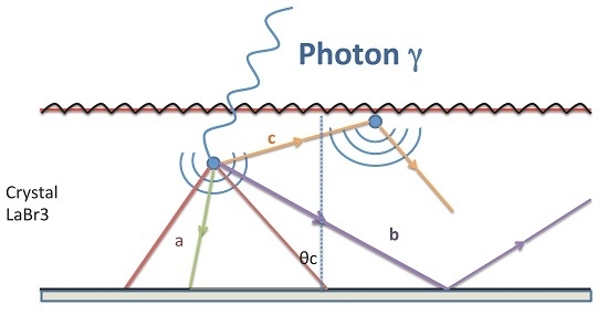
Figure 1) are not scattered and are detected directly. Their path is a straight line to the detector. All the other photons will be subjected to at least one scatter and thus have a longer light path in the crystal, subsequently impacting the photo-detectors.
Between the crystal and the detector, an optical interface with an index step is deployed. Thus, there is a critical angle
above which the photon will be reflected and thus not detected. The unscattered photons will thus be located in a cone whereby the summit is the event position and the opening angle is
. If
is the crystal index and
is the index of the glue between the crystal and the Si-PMT, the critical angle is
. Hence the image of the un-scattered photons on the detector plane will be a disc centered on the location of the interaction
and whose diameter will be
. We can label those un-scattered photons by order of detection on the detector plane, where
will denote the
photon detected with spatio-temporal coordinates on the detector plane
.
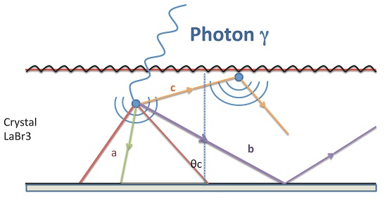
Figure 1 illustrates the behavior of emitted photons after the scintillation event: (a) photons emitted inside the cone are detected directly by the photodetector, (b) photons emitted outside the cone in the downside direction are reflected before being scattered by the upper plane of the crystal, and (c) photons emitted in the upper direction will be scattered in a random direction. Scattering of scintillation photons could also occur in some inclusions inside the crystal. This would create secondary centers of emission in the crystal, mimicking a Compton event. However, both CeBr3 and LYSO are available on the market and have the advantageous property of a very low concentration of scattering imperfections (inclusion is of a size less than 1 mm with a density less than
cm
). Hence, the number of scattered photons, after the first scintillation event, will be below the detection limits in actual systems.
Figure 1.
Illustration of the different behaviors of emitted photons before detection on the Si-PMT: (a) the photons inside the cone are detected; (b) Photons outside the cone and in the downside direction are reflected before being scattered by the diffusive surface and (c) the photons emitted in the upside direction are uniformly scattered when they reach the diffusing surface.
3.1. Simulation of the Images on the Detector Planes
The objective of this subsection is to simulate the spatio-temporal images obtained on the detector plane after a 511 keV photo-electric event. The crystal will be
. Its properties are taken from [
4]. This crystal is selected because it has the highest light field of the commercially available crystals in the emission's first nanosecond. This property is the key success factor for this kind of imagery. As a PET system has been designed by the University of Pennsylvania with LaBr3:Ce [
7], we believe its hygroscopy could be handled. If it is not the case, the concept below would still work with LSO:Ce or LYSO:Ce. The index of the crystal is
for the 380 nm maximum emission. Considering the crystals available for lutetium silicates and LaBr3, the plate described here could have the following dimensions: 100 mm × 250 mm × 30 mm. The crystal has a thickness of 30 mm. The entrance face of the
γ photons is rough and is covered with a white reflector. We will consider this surface as perfectly diffuse in the simulations below (
i.e., the photons striking it are scattered in all directions with an equal probability). The bottom face is polished. Si-PMT is glued to this face with an optical grease with an index of
. The critical angle is then
and the transit time is
ps.
A 511 keV
γ photon enters the crystal and is subject to a photo-electric event located at
. The entrance face is chosen as the reference plane (
). The rise time of this crystal is taken as 750 ps. The UV photons emitted by the photoelectric event are emitted randomly in all 3D directions (
steradian). The emission law
is assumed to be a piecewise function composed of a non-decreasing part between
and
ps and a decreasing function between
and
with a decay time
as follows:
where the parameters
and
are fixed so that the continuity at the time
ps is ensured and so that the total number of emitted photons is equal to 32700 for the 511 keV
γ photon:
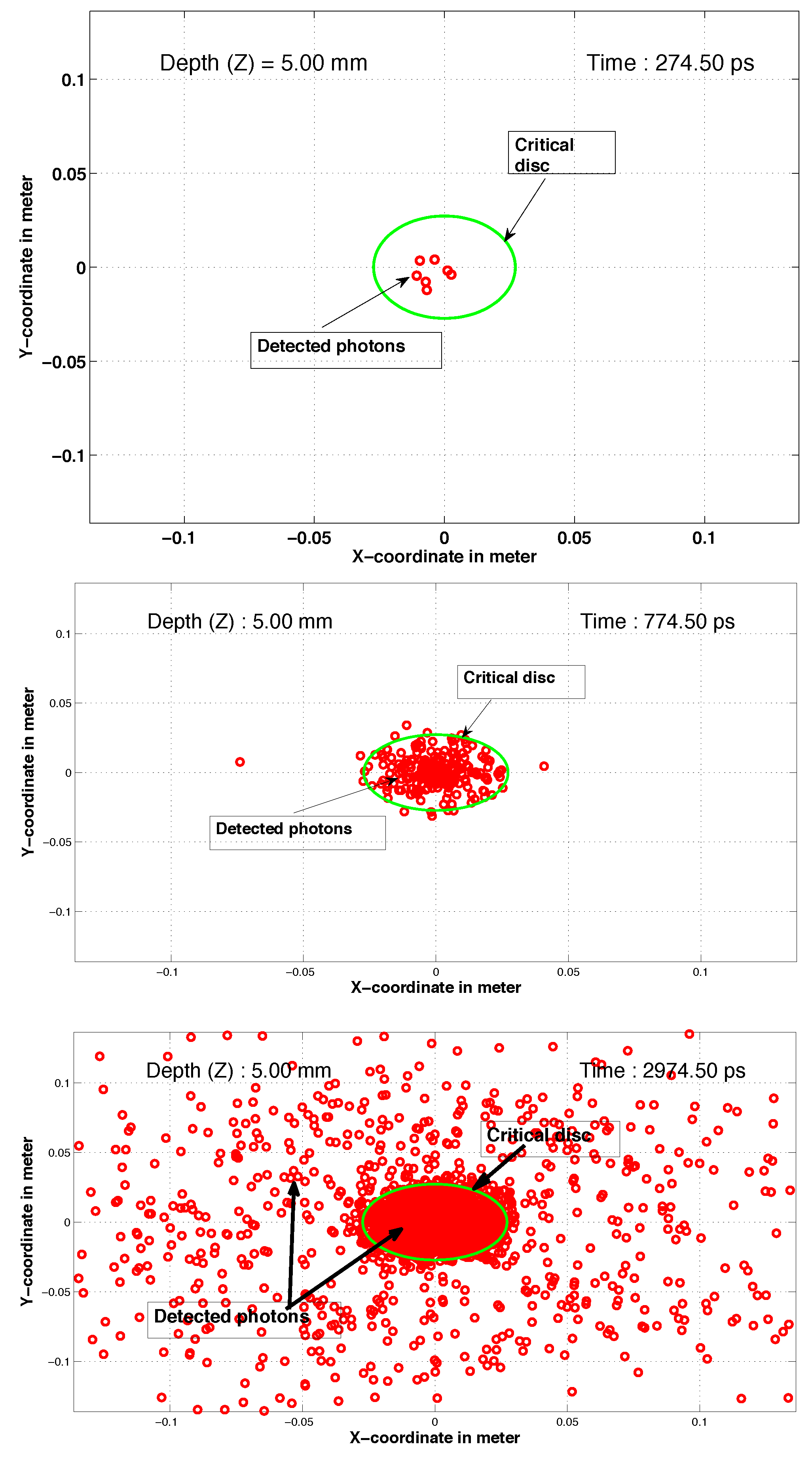
In order to illustrate the temporal behavior of the density of detected un-scattered photons inside the critical disc
(intersection of the critical cone and the detection plane: in green on figures), the images
of detected photons are plotted in
Figure 2 for
mm and different selected time shots (at
ps (100 ps after the detection of the first photon), around the rising time at
ps and around 3 ns). It can be noted that, at the beginning, the first detected photons are inside the critical disc
. Then, the density of photons inside the critical disc increases and a few photons start to appear outside the disc. This behavior is propagated through time: the scattered photons populate the region outside the critical disc, but this later remains highly dense. Note that around the rise time
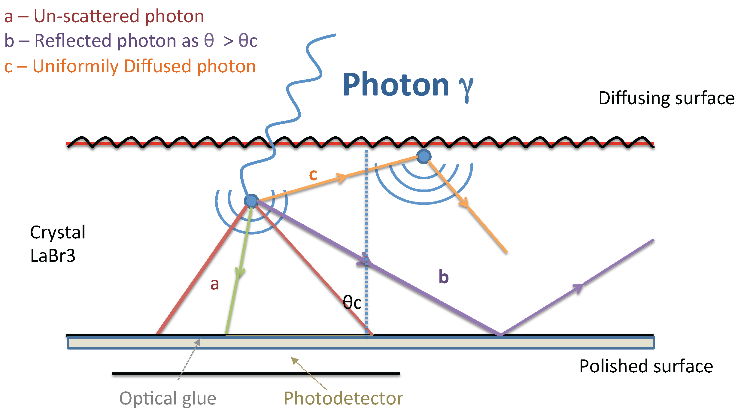
ps, the disc is well filled and only a few photons are outside it. This property will be exploited in the next subsection in order to yield a robust and accurate spatio-temporal localization of the photo-electric event. To further illustrate this property, the evolution through time of the number of detected photons inside and outside the critical disc, as well as their proportion, are reported in
Figure 3a,b respectively. It is worth noting from
Figure 3 that, until 1 ns, at least
of photons are detected inside the critical disc
.
Figure 2.
Images at different time shots for depth Z = 5 mm.
Figure 2.
Images at different time shots for depth Z = 5 mm.
Figure 3.
(a) Number of detected photons inside and outside the critical disc; (b) Percentage of detected photons inside the critical disc.
Figure 3.
(a) Number of detected photons inside and outside the critical disc; (b) Percentage of detected photons inside the critical disc.
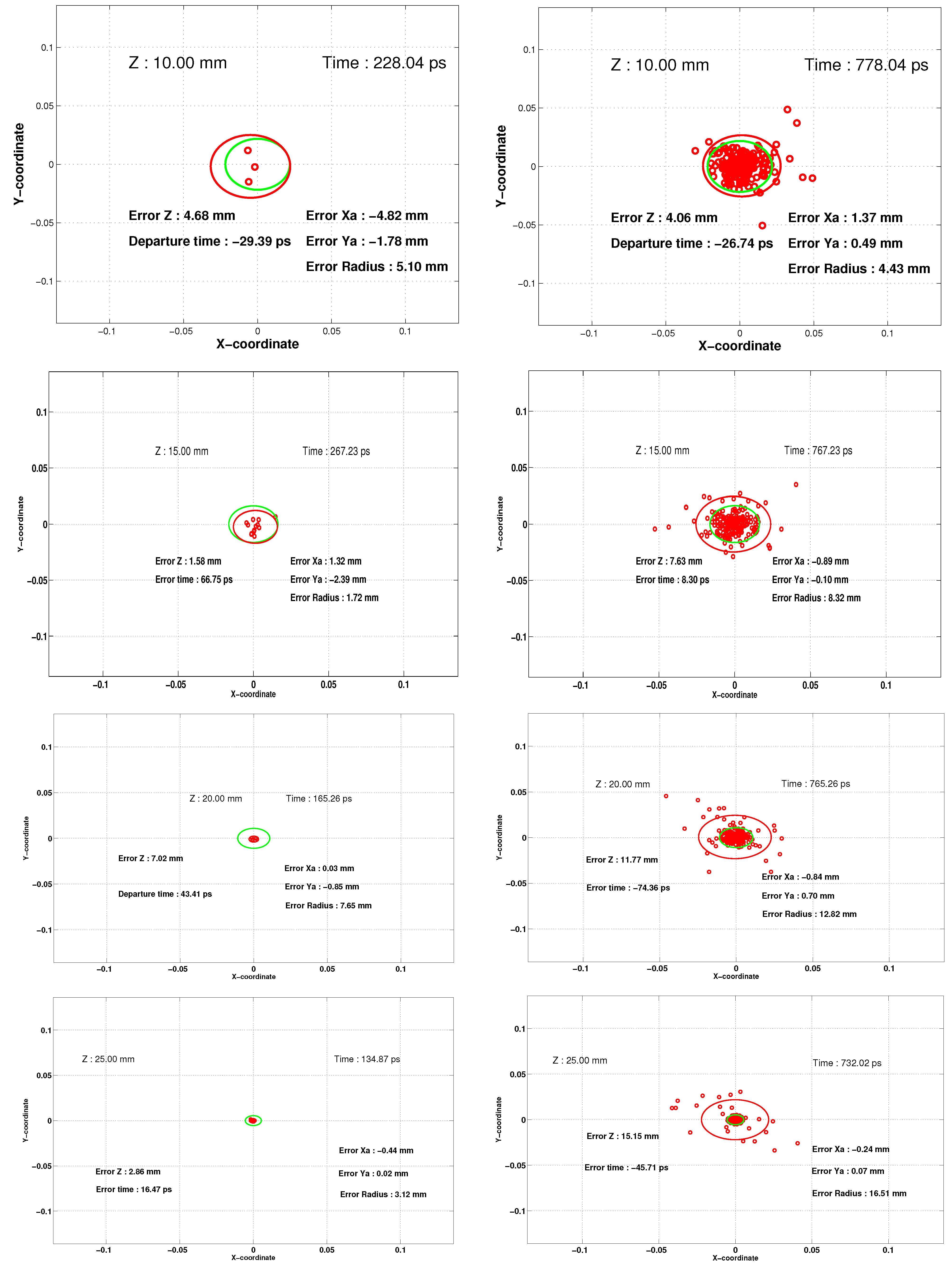
Figure 4 illustrates the temporal images
for each of those different depths
mm,
mm,
mm and
mm. Note that as the depth (
Z) increases, the critical disc gets smaller and more photons are detected outside for the same time shot.
We will briefly discuss now what happens if the absorption of the energy of the Gamma photon is incomplete in the first event, and if a significant Compton scattering is present. The Klein-Nishina formula [
13] shows that for 511 keV photons, most of the energy is partitioned in the forward scattering sector (
i.e.,
). If the scattered photon is diffused at an angle lower than
, the cone of un-scattered photons emitted in case of a photoelectric event will be confined inside the cone of the first event. Thus, all Compton photons scattered at an angle lower than
will not significantly impact the precision of locating the interaction.
3.2. Estimation of the Spatio-Temporal Localization of the Scintillation Event
The critical disc
has the useful property of being quickly filled by the un-scattered photons. The scattered photons may later be detected outside
, which remains, however, highly dense compared to the whole detection plan. Using this property, the 2D spatial localization process consists of first estimating the ellipse containing
of detected photons. The ellipse parameters yield an estimate of the barycenter
and an estimate of the radius
of the critical disc. As the critical angle
is assumed to be known, the estimate
can be deduced by the following relation:
By ray tracing, an estimate of the scintillation time could, in turn, be deduced by considering the time
of the first detected photon at position
. In fact, the trajectory length of the first detected photon is estimated as:
Then, an estimate of the scintillation time
could be deduced as follows:
where
is the photon speed inside the crystal.
Figure 4.
Images at different time shots and different depths. From top to bottom: Z = 10 mm, Z = 15 mm, Z = 20 mm and Z = 25 mm.
Figure 4.
Images at different time shots and different depths. From top to bottom: Z = 10 mm, Z = 15 mm, Z = 20 mm and Z = 25 mm.
The estimation of the spatio-temporal localization
of the scintillation event could be done at any time after the detection of the first incident photon. However, the performance of this estimation varies according to the time chosen for computing the estimates. In fact, the number of detected photons and their spatial distribution evolve in time: at the beginning, only the critical disc is populated by un-scattered photons, but the number of photons remains low to provide a (statistically) robust estimate of the spatio-temporal localization. On the other hand, as the number of detected photons increases with time, the estimation of the ellipse enclosing
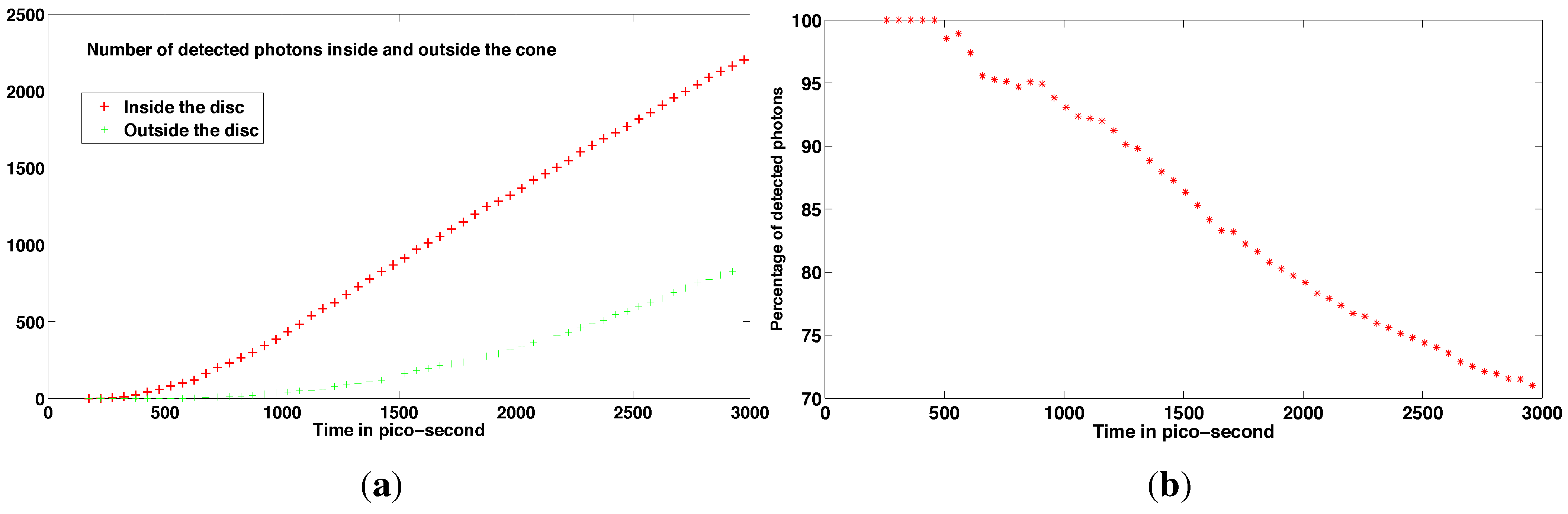
of the points becomes less efficient. In order to illustrate this statement, the absolute error of the
estimates are plotted in
Figure 5a–d, respectively, for the case of depth
mm. Note from
Figure 5a,b, that the estimates of
and
are very accurate with a minimum of
mm error for
X and
mm error for
Y. Also, note the fact that the performance of this estimation does not yield a regular feature through time. However, it can be seen, from
Figure 5c,d, that the precision of the
and
estimates decreases monotonically through time. This is due to the fact that the estimate of the disc radius is less accurate over time. A minimum error of 1 mm for
Z and
ps for
T could be achieved around the rising time of 750 ps.
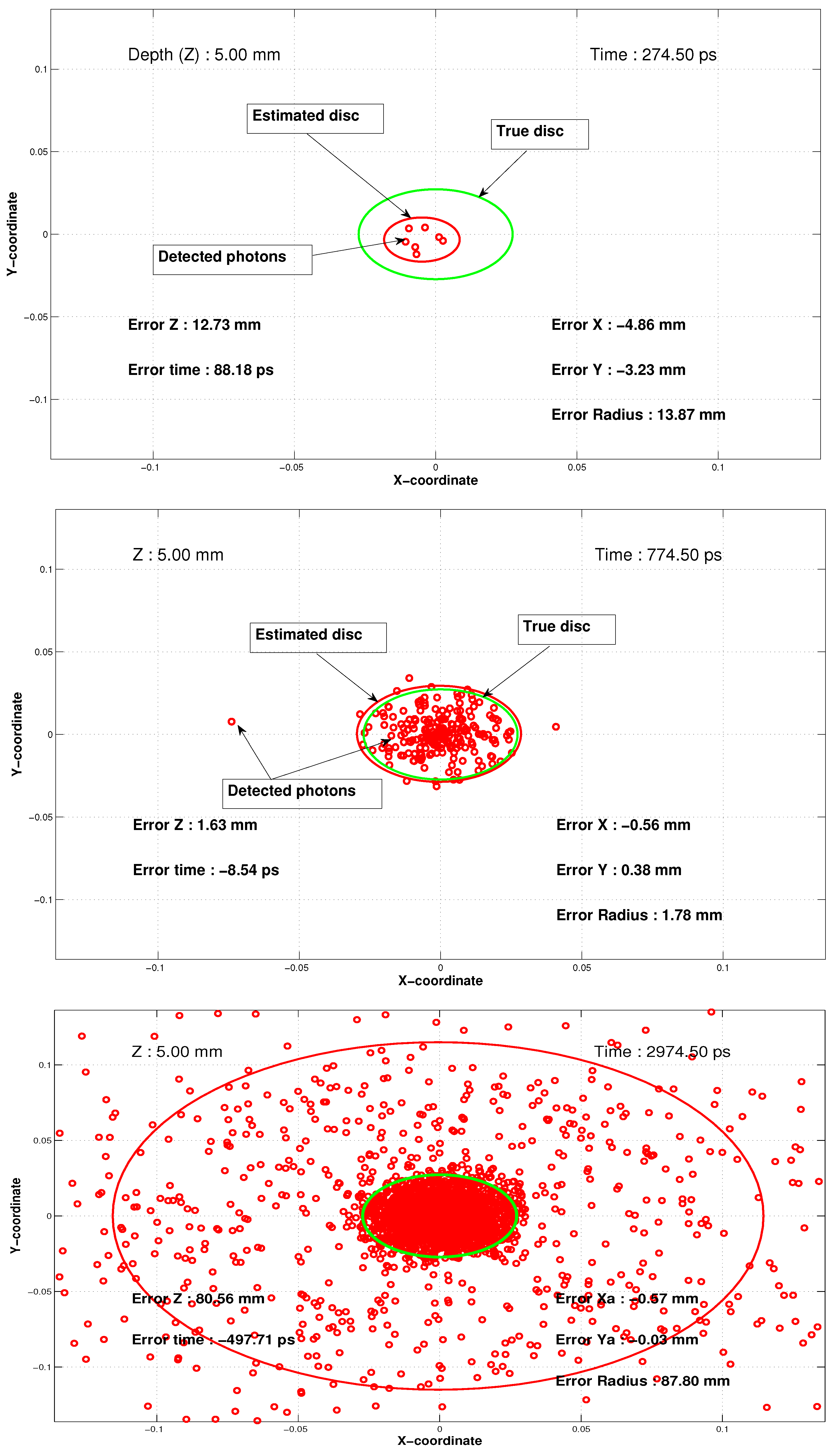
Figure 6 contains the same images as
Figure 2 for 3 selected time shots, but with showing the estimation results and plotting the estimate of the ellipse (approximating the critical disc).
Figure 5.
(a) Absolute error of the X estimate; (b) Absolute error of the Y estimate; (c) Absolute error of the Z estimate and (d) Absolute error of the T estimate.
Figure 5.
(a) Absolute error of the X estimate; (b) Absolute error of the Y estimate; (c) Absolute error of the Z estimate and (d) Absolute error of the T estimate.
In order to confirm the precision of the spatio-temporal localization, Monte Carlo simulations have been conducted. The same algorithm is applied at different depths (
5 mm, 10 mm, 15 mm, 20 mm, 25 mm), each with 10000 simulated data. For each Monte Carlo run, we consider thefollowing assumptions:
Figure 6.
Images at different time shots and corresponding estimation results for 5 mm depth; true disc is plotted in green and estimated disc in red.
Figure 6.
Images at different time shots and corresponding estimation results for 5 mm depth; true disc is plotted in green and estimated disc in red.
The photons’ directions, after the scintillation event, are sampled according to a uniform distribution in all 3D directions.
The detection of un-scattered photons is considered as deterministic. In other words, if incident UV photons have an angle lower than the critical angle , they are considered as detectable by the Si-PM. However, detection efficacy is considered as follows: only a percentage of incident photons are considered as effectively detected. However, this random detection does not affect the property of the spatial distribution of the detected photons: the region inside the critical disc has a higher density than the whole plane.
The reflection on the lower detector plane is considered as deterministic: the incident photon with an angle higher than is reflected with the same angle.
The scattering on the upper plane is considered as random, with a uniform distribution in all 3D directions. A random absorption of the incident photons on the upper surface is also considered.
These Monte-Carlo simulations are implemented with Matlab software, considering simple yet realistic physical assumptions about the scintillation event, the propagation of UV photons, the reflection on the polished surface and the scattering on the upper crystal surface. The Compton effect is not considered in these Monte Carlo simulations. However, as explained above, according to the Klein-Nishina formula, the density of the critical disc is expected to remain higher than the whole plane. The use of the discontinuity of the critical disc is then not affected.
For each depth
Z, an optimal decision time exists (time when the estimates could be optimally computed). However, as the depth is
a priori unknown, one has to set a decision time which will be considered independently of the actual depth. The setting of the decision time should be done while considering the trade-off between 2 aspects: (i) the error on T and Z grows over time and (ii) the statistical robustness of the ellipse estimation increases as the number of detected photons increases.
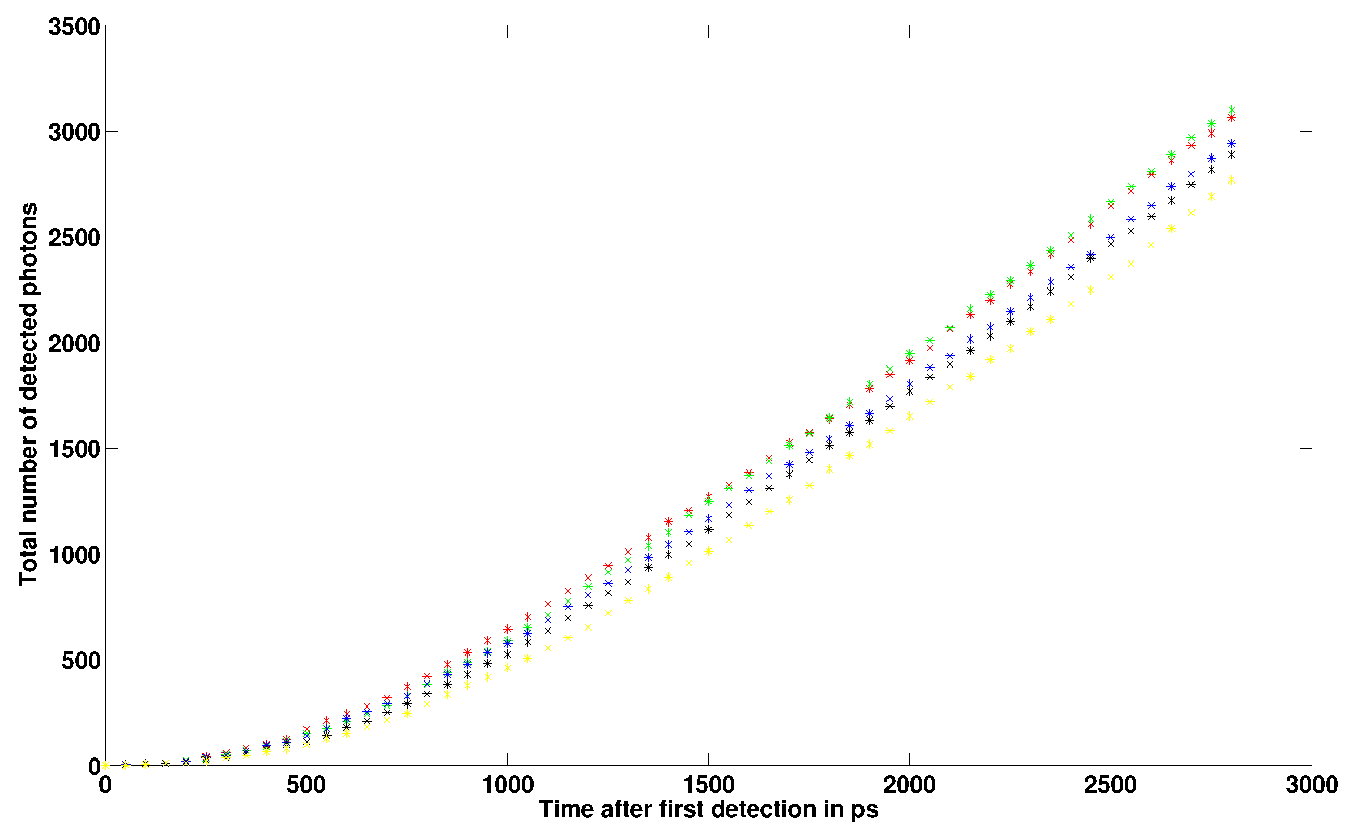
Figure 7 shows the total number of detected photons over time for different depths. It is clear that greater depth results in a lower number of photons.
Figure 7.
Total number of detected photons for various depths: 5 mm (red), 10 mm (blue), 15 mm (magenta), 20 mm (black), 25 mm (cyan).
Figure 7.
Total number of detected photons for various depths: 5 mm (red), 10 mm (blue), 15 mm (magenta), 20 mm (black), 25 mm (cyan).
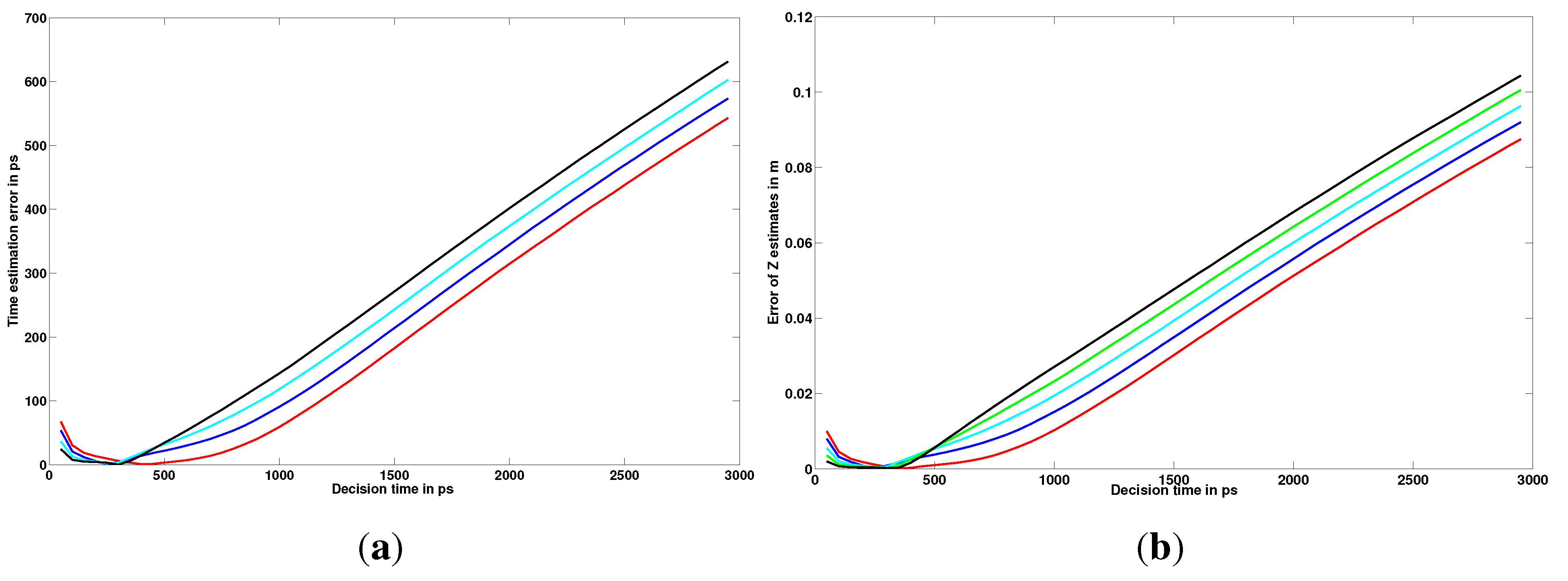
On the other hand,
Figure 8a shows the evolution of time estimation error with respect to the decision time (Monte Carlo average) and
Figure 8b shows the evolution of Z estimation error with respect to the decision time (Monte Carlo average). It is worth noting that the time error has the same behavior: first, it decreases reaching its minimum (which decreases as
Z increases) and then it increases in a monotone way. Consequently, a practical choice of the decision time could be between 500 ps and 750 ps as the number of detected photons is at least 100, which ensures the robustness of the statistical estimation of the critical disc.
Figure 8.
(a) Absolute error of the T estimate (in picoseconds) for various depths: 5 mm (red), 10 mm (blue), 15 mm (cyan), 20 mm (green), 25 mm (black); (b) Absolute error of the Z estimate (in meters) for many depths: 5 mm (red), 10 mm (blue), 15 mm (cyan), 20 mm (green), 25 mm (black).
Figure 8.
(a) Absolute error of the T estimate (in picoseconds) for various depths: 5 mm (red), 10 mm (blue), 15 mm (cyan), 20 mm (green), 25 mm (black); (b) Absolute error of the Z estimate (in meters) for many depths: 5 mm (red), 10 mm (blue), 15 mm (cyan), 20 mm (green), 25 mm (black).
In
Table 1, the Monte Carlo estimation errors of the spatio-temporal localization are reported for different depths at a decision time
ps (after the first photon detection).
Table 1.
Monte Carlo averages of absolute errors of X, Y, Z (in mm) and T (in ps) for different depths of the scintillation event. Decision time is taken 700 ps after the first photon detection.
Table 1.
Monte Carlo averages of absolute errors of X, Y, Z (in mm) and T (in ps) for different depths of the scintillation event. Decision time is taken 700 ps after the first photon detection.
| | | | | |
|---|
| Z = 5 mm | 0.0042 | 0.01 | 2.8 | 10.3 |
| Z = 10 mm | 0.0031 | 0.03 | 4 | 35.07 |
| Z = 15 mm | 0.017 | 0.002 | 6.3 | 52.47 |
| Z = 20 mm | 0.0142 | 0.02 | 9.3 | 64.72 |
| Z = 25 mm | 0.0009 | 0.01 | 12 | 75.95 |
In order to compare the performances of the proposed temporal imager with the state-of-the-art LYSO detectors,
Table 2 shows the spatio-temporal localization precision and the energy resolution of both systems. The gain in performances can be seen at all levels: 2D coordinates (X,Y), depth of interaction (Z), timing of interaction (T) and also the energy resolution which can be lower than
. In the same table, we have also compared the performances of the proposed temporal imager with two different crystals having different physical properties: CeBr3 and LYSO. The CeBr3 crystal shows better results.
Table 2.
Comparison of the proposed temporal imager performances with the state-of-the-art LYSO system.
Table 2.
Comparison of the proposed temporal imager performances with the state-of-the-art LYSO system.
| | Today (Pixels LYSO) | Temporal Imager CeBr3 | Temporal Imager LYSO |
|---|
| X, Y | 5 mm | <1 mm | <1 mm |
| Z | 20 mm | <5 mm | <5 mm |
| T | 600 ps | <100 ps | <150 ps |
| Energy | 12 %–15 % | <5 % | <5 % |


