1. Introduction
Ultrasound scanning is a widely-used modality in healthcare, as it provides real-time, safer and noninvasive imaging of organs in the body, including heart, kidney, liver, fetus,
etc. Conventional ultrasound machines cannot be used for point-of-care (POC) applications due to their high form factor. POC refers to treating the patients at their bedside, which has great potentiality in saving lives, especially in situations like ambulances, military, casualties, rural healthcare,
etc.[
1]. Ultrasound scanning needs limited setup for scanning, and advancements in computing platforms enable portable ultrasound scanning (PUS) systems’ use in POC applications.
Commercially-available PUS with application-specific integrated circuit (ASIC) cannot be updated with new algorithms, while programmable ultrasound scanning machines provide the flexibility for rapid prototyping, updating and validating new algorithms [
2]. Computing platforms, such as field-programmable gate array (FPGA), digital signal processor (DSP) and media processors, have capabilities in terms of hardware to realize complex ultrasound signal processing algorithms in real time. In [
3], ultrasound signal processing is performed on a single media processor; due to the computational limitations of the processor, the beamformed data are acquired through an ultrasound research interface from a high-end system, and the real-time mid-end and back-end processing algorithms are implemented on a media processor. In [
4], a complete standalone ultrasound scanning machine is realized using single FPGA and a proposed pseudo-dynamic received beamforming with an extended aperture technique targeting the PUS system. In [
5], we proposed a low complexity programmable FPGA-based eight-channel ultrasound transmitter for research, which enables rapid prototyping of new algorithms. ASIC for ultrasound signal processing is beneficial for reducing the size of the ultrasound machine, and we proposed an ASIC design for integrated transmit and receive beamforming in [
6]. In [
7], the authors demonstrated the feasibility of implementing the ultrasound signal processing on a high-end android mobile platform. Low complexity algorithms have been proposed for portable ultrasound machines, such that they can be easily implemented on computational platforms that have less computational capability [
8,
9,
10,
11].
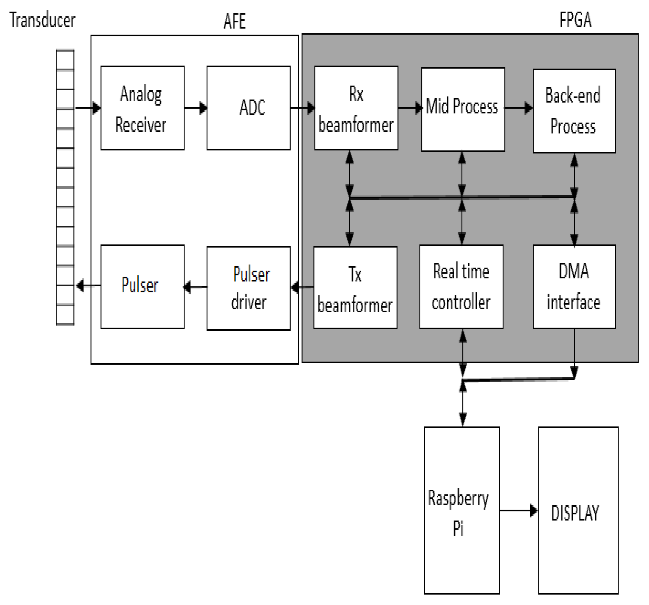
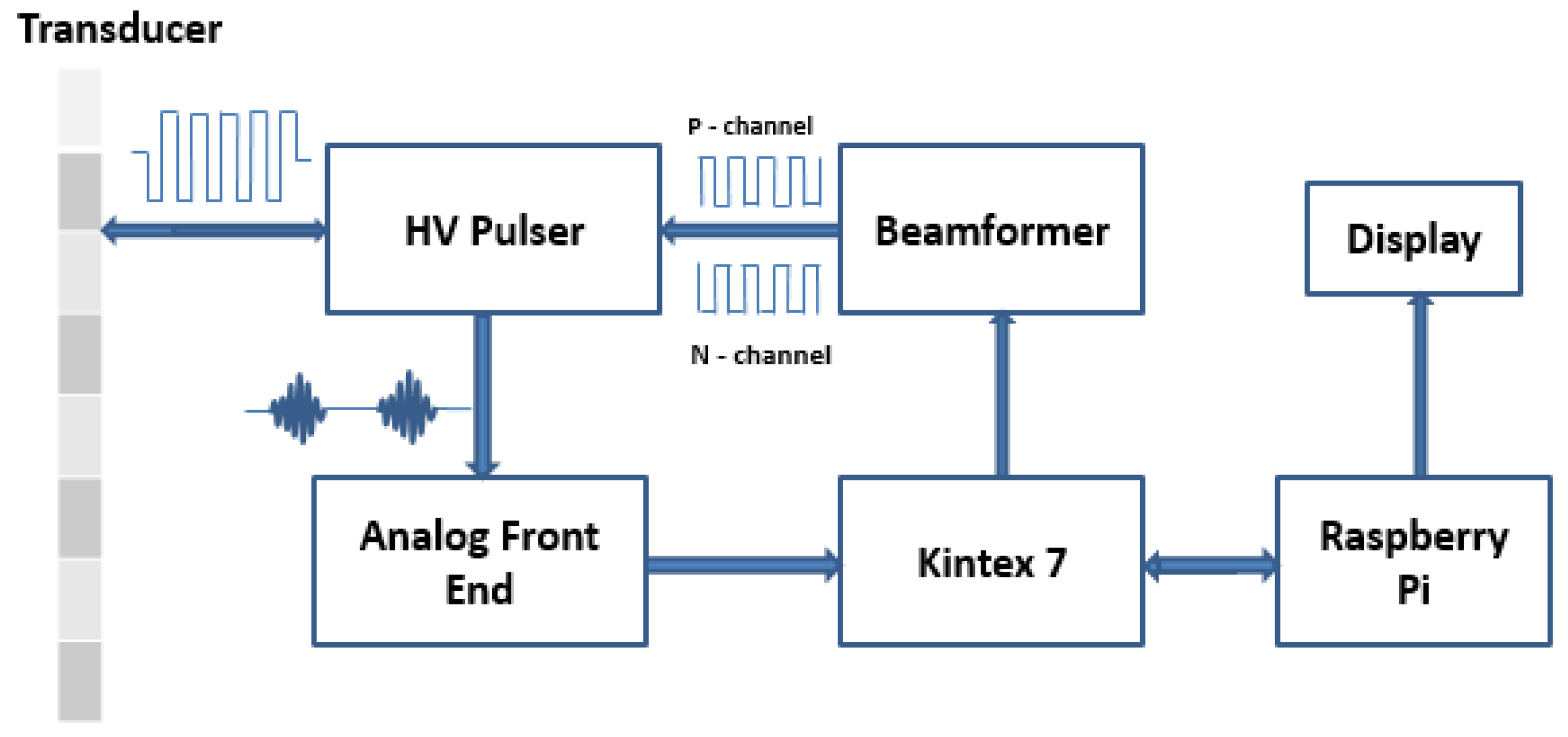
In this paper, we propose an FPGA-based standalone portable ultrasound scanning system with real-time kidney detection. We chose FPGA for implementing complete ultrasound signal processing due to its efficiency in handling high data rates. The PUS machine is realized using Kintex-7 [
12], which is integrated with an ARM1176JZF-S Raspberry Pi-2 processor [
13].
For displaying and recording the scanned ultrasound data, the H.264 codec is used. H.264 is a computationally-expensive procedure, and several optimized versions are proposed to implement in real time on different computing platforms, like FPGAs, DSPs, microprocessors,
etc. Here, we list some of the optimizations proposed for the H.264 codec to implement on an FPFA platform. In [
14], low complexity and low energy adaptive hardware for H.264 with multiple frame reference motion estimation is proposed and implemented on an FPGA platform. A bioinspired custom-made reconfigurable hardware architecture is proposed in [
15,
16] for efficient computation of motion between image sequences. The work in [
17] proposed a flexible and scalable fast estimation processor targeting the computational requirements for high definition video using the H.264 video codec on an FPGA platform. Optimization for accelerating the block matching algorithms on a Nios II microprocessor, which is designed for FPGA, is proposed in [
18,
19]. A new early termination algorithm is proposed in [
20] for effective computation of the correlation coefficient in template matching with fewer computations. Several optimizations are available for implementing the H.264 codec on an FPGA, but the FPGA resources in the proposed portable ultrasound system are preserved for implementing complex Doppler ultrasound. In the proposed portable ultrasound system, the H.264 codec is installed on a Raspberry Pi processor, which is downloaded from [
21].
Even though ultrasound scanning is widely used, the ultrasound images have a low signal-to-noise ratio and contrast, and there will not be any significant distinction between the organ region and edges, making it difficult to identify the organ exactly. Portable ultrasound scanners in remote areas are mostly used by emergency physicians who may not be fully trained in sonography. Hence, there is a need for computer-assisted algorithms, which can assist physicians in making accurate decisions. These algorithms include speckle suppression, organ detection, computer-aided diagnosis (CAD), etc. Hence, automatic detection will be very beneficial for the development of applications related to CAD, image compression, segmentation, image-guided interventions, etc.
In the literature, portable ultrasound scanning machines are realized on FPGAs, DSPs and media processors [
2,
3,
4], and the automatic detection of kidneys in CT images based on random forest is proposed. The algorithms proposed for CT images will not work for ultrasound images, as the characteristics of kidney change with imaging modality, and the kidney images acquired through ultrasound scanning depend on the person who scans. Therefore, manual cropping is employed for detecting the kidney in ultrasound images [
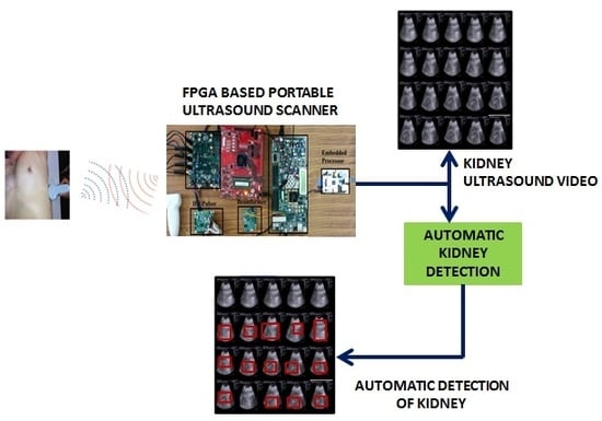
22]. In this paper, we propose an automatic kidney detection algorithm for detecting the kidneys in a real-time ultrasound video and evaluate the algorithm on an FPGA-based PUS machine in real-time. To the best of our knowledge, this is the first working prototype of a portable ultrasound scanner with automatic detection of kidney. The prototype of the PUS is evaluated by scanning the tissue-mimicking gelatin phantom. The reconstructed images of the PUS are visually compared to the images of commercially available platforms. The proposed portable ultrasound scanner with the kidney detection algorithm is successfully tested at the lab level.
The rest of the paper is organized as follows. In
Section 2, we describe the flow adhered to for automated kidney detection. The hardware implementation of the portable ultrasound system is described in
Section 3. The experimental setup and performance of the system are discussed in
Section 4.
Section 5 concludes the paper with discussions on the future scope of work.
2. Automatic Kidney Detection
Automatic organ detection is very beneficial for semi-skilled persons who operate the device remotely. Organ detection in ultrasound is strongly influenced by the quality of data. The characteristic artifacts that make the organ detection complicated are speckle noise, acoustic shadows, attenuation, signal dropout and missing boundaries of the organ. In this paper, we focus on detecting kidney in ultrasound images, which is different from segmentation of kidney, i.e., extracting the exact contour of kidney. Kidney is made up of soft tissue, and it is nonrigid in nature. Moreover, the size of kidney in ultrasound images varies from patient to patient depending on the patient’s age, anatomy, disease, orientation of acquisition, etc., so, it becomes a challenging task to automatically detect kidney in ultrasound images.
In the literature, the problem of automatic detection of kidney with ultrasound images has never been addressed before. However, there are some algorithms proposed in the literature to segment the kidney in ultrasound. Automatic organ detection is addressed as one of the intermediate steps involved in the segmentation procedure. Organs have to be accurately segmented in designing applications, like 3D reconstruction, CAD, automatic measurements,
etc. Organ detection and localization are the two major steps involved in segmentation. In the literature, not much interest is shown in automatic detection of organs, while major research is done on detecting the exact contour of an organ. The organs in the images are detected by manually cropping along the contours [
22], placing the landmarks on the contour [
23] and marking the bounding boxes around the kidney [
24]. Automatic detection of kidney in CT slices using random forest has been used in [
25] for reconstructing the 3D structure of kidney. A two-stage detection algorithm is employed for automatic detection of lymph nodes in CT data; Haar features with the Adaboost cascade classifier are used in the first stage, and in the second stage, self-assigning features with the Adaboost cascade classifier are used [
26]. The algorithm proposed in [
22] needs manual cropping and assumes that kidney is present in every slice. However, when we scan kidney using 2D probes, we cannot expect kidney to be present in each frame, and kidneys also have been occluded by surrounding organs, like liver and spleen. As kidney is not present in every slice, the correlation between two frames is not useful in tracking the kidney. Therefore, the algorithm has to detect the kidney in each incoming slice. The kidney detection algorithm has to be fast enough at automatically detecting the kidney in real time from incoming ultrasound data.
Active contours [
27], also known as snakes [
28], pose contour detection as an optimization problem that moves a parameterized curve towards the image region with strong edges; though this model is highly successful, it suffers from initialization, and the optimization function being nonlinear, as a result, the solution is trapped in many places. In level-set methods [
29,
30], the contour of kidney is represented by a level-set zero of a distance function; this approach is less sensitive to initialization and significantly suffers from imaging conditions. Both active contours and level-set approaches are highly successful in contour extraction; they present the drawback of incorporating prior knowledge about the shape and texture distribution in the optimization function; the prior knowledge may be in the form of a probability distribution formed from the manually-segmented contours and textures. Active shape models (ASM) [
23] and active appearance models (AAM) [
31] are supervised learning approaches, which estimate the parameters from a joint distribution representing the shape and appearance of an organ; these methods need large databases, and the initialization of the contour should be close to local optima. In [
32], kidney segmentation based on texture and shape priors is proposed; the texture features are extracted from a bank of Gabor filters on test images, then an iterative segmentation is proposed to combine texture measures into a parametric shape model. In [
22], a probabilistic Bayesian method is employed to detect the contours in a three-dimensional ultrasound.
The models discussed above are constraint based on the terms of shapes and the condition of the organ (normal and abnormal). For example, active contours will fail to extract the exact contour of kidney in the presence of cysts in kidney. However, the ASM and AAM can capture the contour of kidney even in the presence of cysts, but fail to capture the diversified variations of contour. In this paper, we are interested in detecting the region of interest for kidney, which is useful to emphasize only that particular region further. The method we adopted for detecting kidney in an ultrasound images is based on a Viola–Jones detector [
33]. Viola–Jones is highly successful in detecting many object classes; it was primarily developed for face detection in images and later extended to detect faces in video sequences [
34]. Recently, the Viola–Jones algorithm framework was used in medical image analysis to detect various organs, such as pelvis and proximal femur of a hip joint in 3D CT images [
35]. In [
36], a modified Viola–Jones algorithm is used to automatically locate the carotid artery in ultrasound images.
In this paper, we show the effectiveness of the Viola–Jones algorithm in detecting the region of interest for kidney in ultrasound images. The complete Viola–Jones algorithm is implemented on a Raspberry pi board, which is interfaced with the Xilinx Kintex-7 FPGA, where ultrasound signal processing algorithms are implemented.
The block diagram representation of the kidney detection algorithm is shown in
Figure 1. The basic components corresponding to this algorithm include Haar-like features, the integral image, the Adaboost algorithm and the cascade of classifiers.
Figure 1.
Block diagram of the Viola–Jones algorithm for detecting kidney.
Figure 1.
Block diagram of the Viola–Jones algorithm for detecting kidney.
2.1. Haar-Like Features Used in the Kidney Detection Algorithm
Haar-like features are derived from the kernels [
37]; a few of these kernels are shown in
Figure 2. The white region in the kernel corresponds to weight
, and the black region corresponds to
. The value of these features are then computed using the formula
, where
is the response of a given Haar-like feature to the input image
x,
is the weight of the area
and
is the weight of the black area
. The number of pixels in areas
and
varies because the features are generated for various possible combinations and positions in a given window. These dimensions start from a single pixel and extend up to the size of a given window.
Figure 2.
Kernels used to extract Haar-like features for the kidney detection algorithm. (a,b) Two-rectangle features. (c,d) Three-rectangle features and (e) Four-rectangle feature.
Figure 2.
Kernels used to extract Haar-like features for the kidney detection algorithm. (a,b) Two-rectangle features. (c,d) Three-rectangle features and (e) Four-rectangle feature.
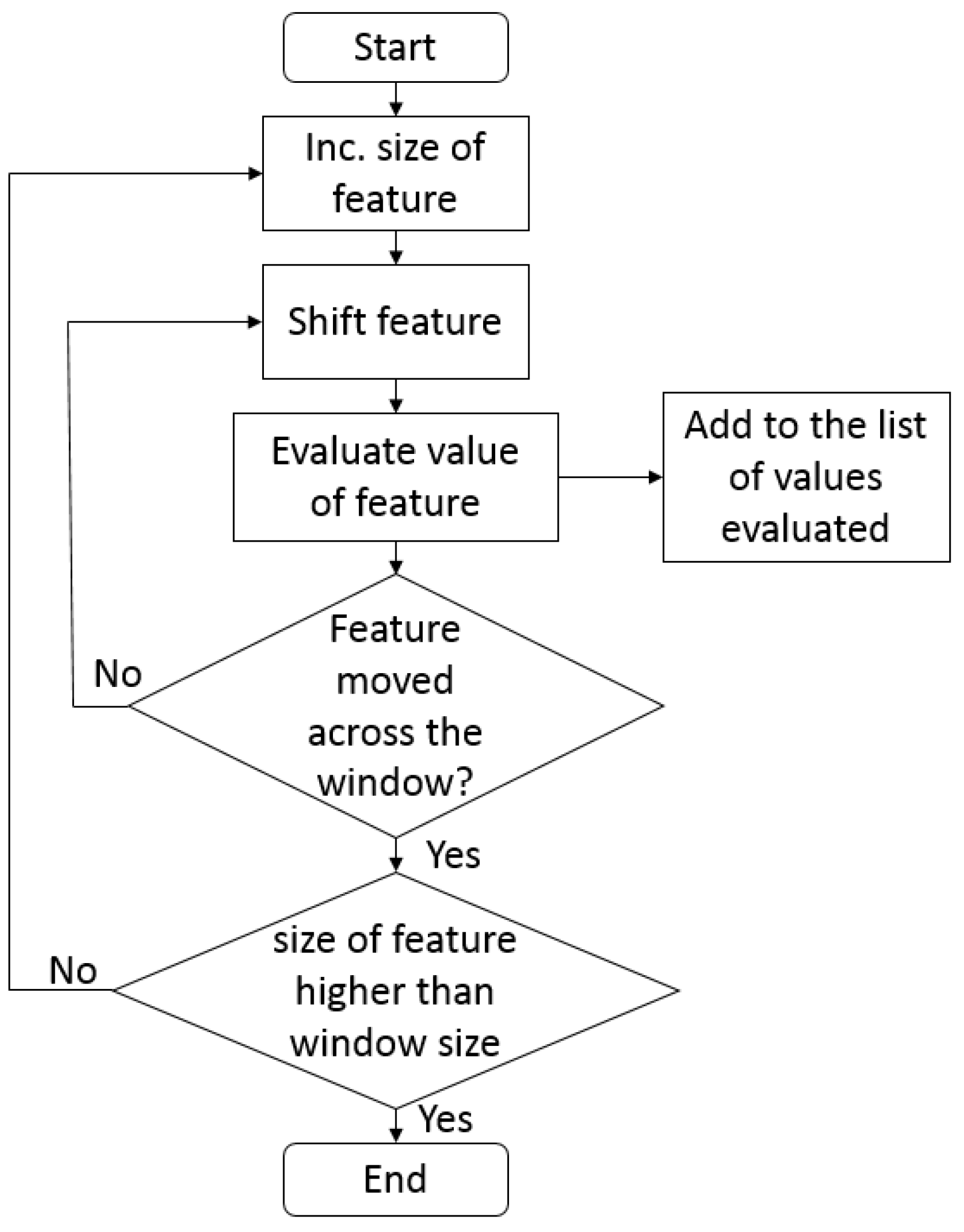
The features generated using these kernels are independent of image content. The process of feature generation is explained as follows: considering the kernel in
Figure 2a, which is initially of a two-pixel column width (one pixel white and one pixel black), the feature value of
is computed. The kernel is shifted from the top left of the image by one pixel, and a new feature value is calculated. Similarly, the kernel is then moved across the complete image, until it reaches the right bottom of the image with all of the features computed. Hence, the features are evaluated hundreds of times as the kernel moves across all of the rows of the image, and every time, a new feature value is updated in the feature list. Later, the kernel is increased to a four-pixel width (two white pixels and two black pixels), and the process is repeated to get new feature values. Five different kernels are used for generating the rectangular features. The process is repeated for all of the kernels; considering all of the variations in size and position, a total of 586,992 features were computed [
33] for a window of size 32 × 54 [
38].
Figure 3 illustrates the flowchart for generating Haar-like features.
Figure 3.
Flowchart to generate Haar-like features for the kidney detection algorithm.
Figure 3.
Flowchart to generate Haar-like features for the kidney detection algorithm.
2.2. Integral Image
Computing the sum of pixels in a given area is a computationally-expensive procedure; hence, intermediate representation of the image is used to compute the features rapidly and efficiently; this representation of the image is called an integral image [
39]. The conversion of the image to an integral image is based on the following formulae:
where
u,
v are the indices of the pixel,
is the cumulative sum of pixel values in a row with initial conditions as
and
,
is the pixel value of original image and
is the pixel value of the integral image.
In the integral image, the sum of all pixels under a rectangle can be evaluated using only the four-corner values of the image, which is similar to the summed area technique used in graphics [
40]. In
Figure 4, the value of the integral image at Location 1 is the sum of pixels in Rectangle A, at Location 2 A + B, at Location 3 A + C and at Location 4 A + B + C + D. The sum of pixels in D can be evaluated as (4 + 1) − (2 + 3).
Figure 4.
Sum of the pixels in Region D using the four-array reference.
Figure 4.
Sum of the pixels in Region D using the four-array reference.
2.3. Selection of Features for Automatic Kidney Detection Using the Adaboost Algorithm
Adaboost is a machine learning algorithm that helps with finding the best features among 586,000+ features [
41,
42] for detecting kidney. After evaluating the obtained features from the Adaboost algorithm, the weighted combination of these features is used to decide whether a given window has kidney or not. These selected features are also called weak classifiers. The output of a weak classifier is binary, either one or zero. One indicates that the feature is detected in the window, and zero indicates that there is no feature in the window. Adaboost constructs a strong classifier based on the linear combination of these weak classifiers.
where
is a strong classifier,
is a weak classifier and
is the weight corresponding to the error evaluated using classifier
.
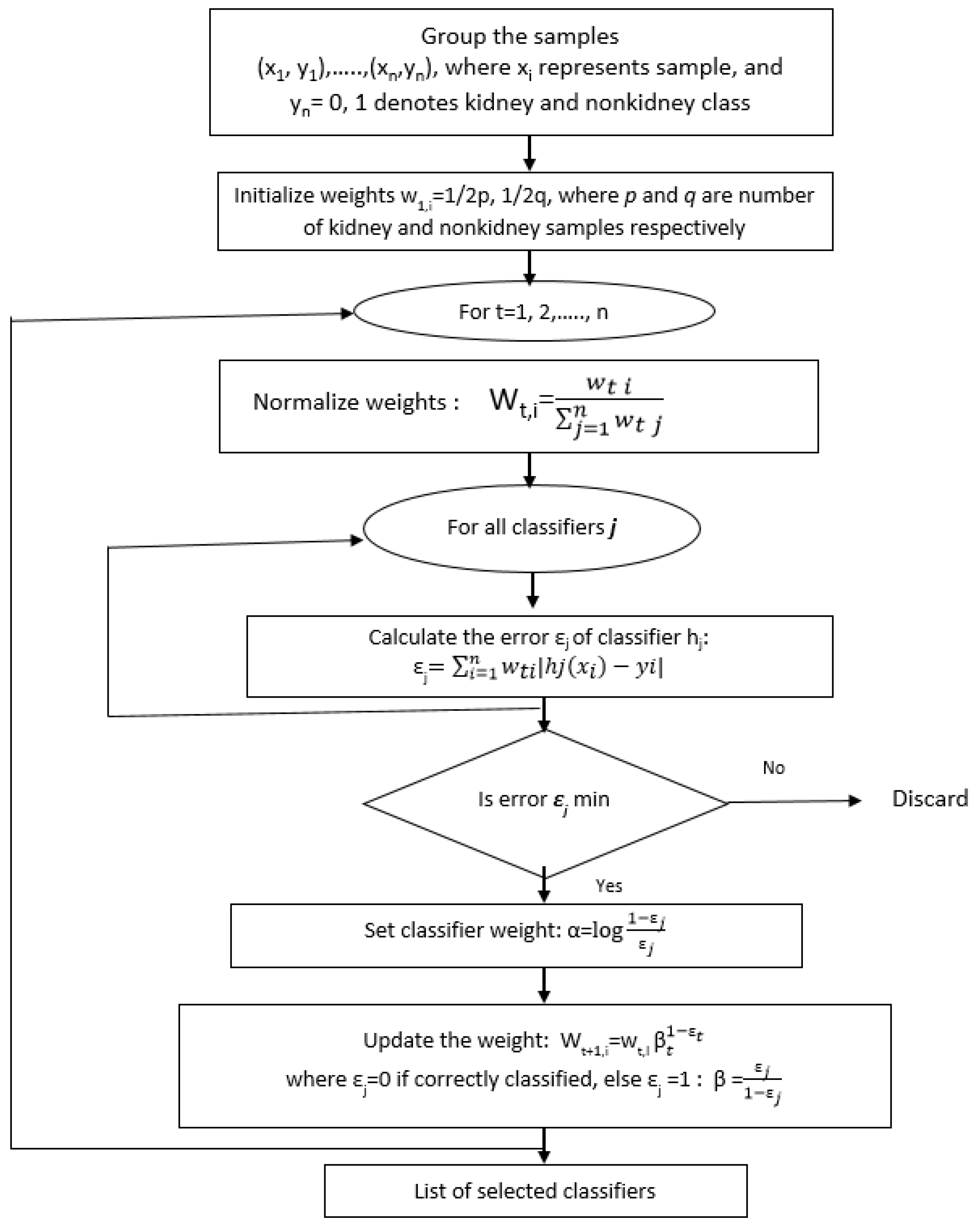
The flowchart for computing the features using the Adaboost algorithm is shown in
Figure 5 [
36]. Adaboost starts with a uniform distribution of weights over training examples. The classifier with the lowest weighted error (a weak classifier) is selected. Later, the weights of the misclassified examples are increased, and the process is continued, till the required number of features is selected. Finally, a linear combination of all of these weak classifiers is evaluated, and a threshold is selected. If the linear combination of a new image in a given window is greater than this threshold, it is considered as kidney being present; if it is less than the threshold, it is classified as non-kidney. The Adaboost algorithm finds a single feature and threshold that best separate the positive (kidney) and negative (non-kidney) training examples in terms of weighted error. Firstly, the initial weights are set for positive (with kidney) and negative (without kidney) examples. Each classifier is used from 586,000+ features to determine the error, which in this case is to misclassify the presence of kidney in a window. If the error is high, the training process ends; else, the weights
are set to the selected linear classifier. The
are computed as:
where
is the error occurring while classifying the images. Later, the weights of the positive and negative examples are adjusted, such that the weights of the misclassified examples are boosted, and the weights of the correctly-classified examples are not changed. Finally, a strong classifier is created, which is a combination of weak ones weighted according to the error that they had.
Figure 5.
Flowchart of the Adaboost algorithm for selecting the features for kidney detection.
Figure 5.
Flowchart of the Adaboost algorithm for selecting the features for kidney detection.
2.4. Cascade Classifier for Automatic Kidney Detection
The strong classifier formed from the linear combination of these best features is a computationally-expensive procedure. Therefore, a cascade classifier is used, which consists of stages, and each stage has a strong classifier [
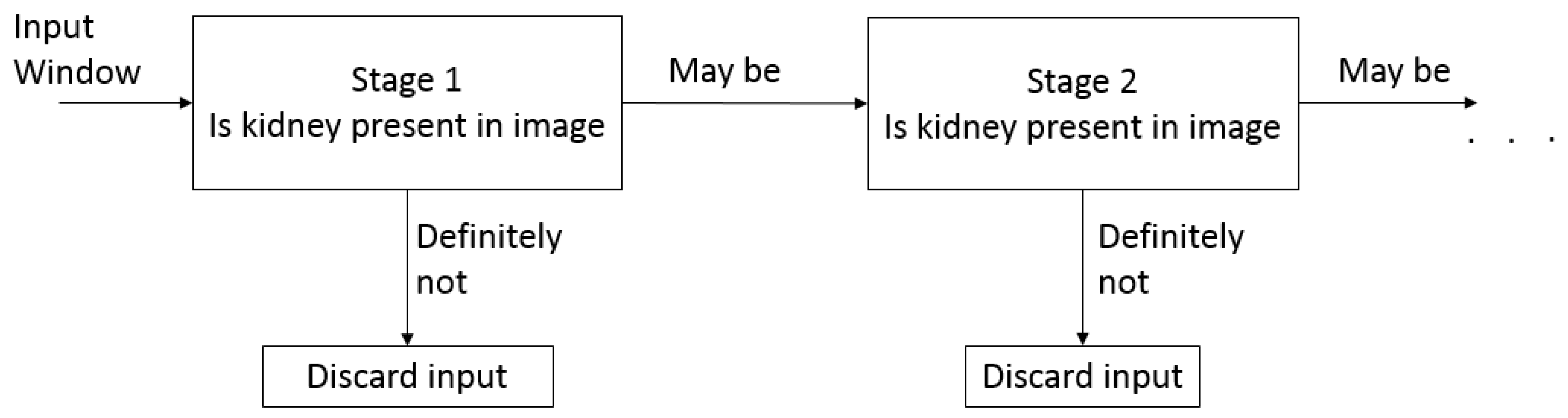
43]. Therefore, all of the features are grouped into several stages, where each stage has a certain number of features along with a strong classifier. Thus, each stage is used to determine whether a kidney is present in a given sub-window. The block diagram of the cascade classifier is shown in
Figure 6. A given sub-window is immediately discarded if kidney is not present and not considered for further stages. The cascade classifier works on the principle of rejection, as the majority of sub-windows will be negative. It rejects many negatives at the earliest stage possible. This reduces the computational cost, and hence, kidney in the image can be detected at a faster rate. The complete analysis and implementation of the Viola–Jones algorithm can be found in [
44].
Figure 6.
Block diagram of the cascade classifier for kidney detection.
Figure 6.
Block diagram of the cascade classifier for kidney detection.
2.5. Database
Kidney images and videos were acquired using a Siemens S1000 from 400 patients during the period May 2014 to February 2015. These patients were in the age group of 14 to 65 years, including both genders. The database consists of 790 images with 400 kidney (normal: 332; cyst: 40; stone: 28) and 390 non-kidney (liver: 100; heart: 95; carotid: 90; spleen: 105) images. The kidney and non-kidney images were collected from the same patients. The data were collected by acknowledging the patients. The data received from the doctor were annotated with the patient’s age, gender and disease. The names of the patients were not revealed in the process.
2.6. Metrics Used for Evaluating the Automatic Kidney Detection Algorithm
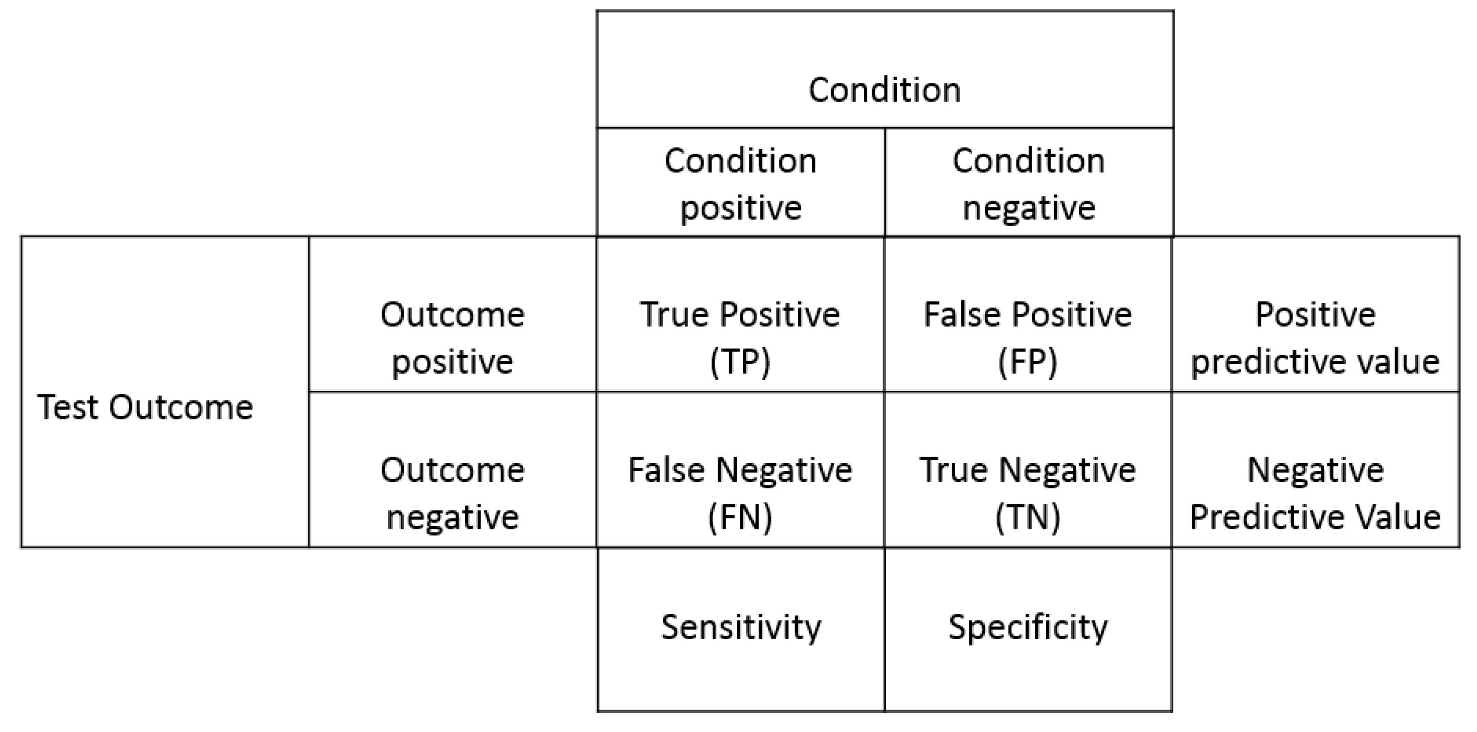
The performance of the organ detection algorithm is evaluated by tabulating the confusion matrix. The metrics used in this paper, referring to
Figure 7, are given below:
Figure 7.
Confusion matrix.
Figure 7.
Confusion matrix.
Sensitivity measures the proportion of actual positives, and specificity measures the proportion of actual negatives correctly identified as such, respectively. A positive predictive value measures the efficiency of an algorithm to correctly identify normal kidneys, and a negative predictive value measures the efficiency of an algorithm to correctly identify negative images. Accuracy gives the efficiency of an algorithm in correctly localizing kidney in the images.
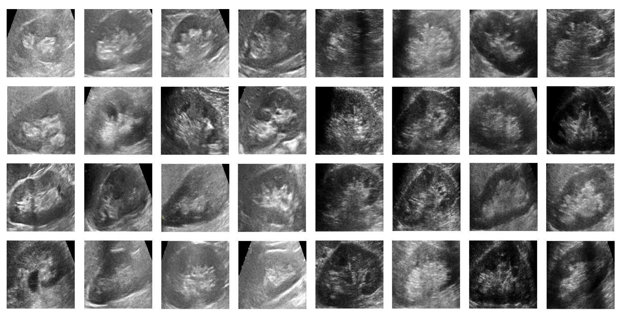
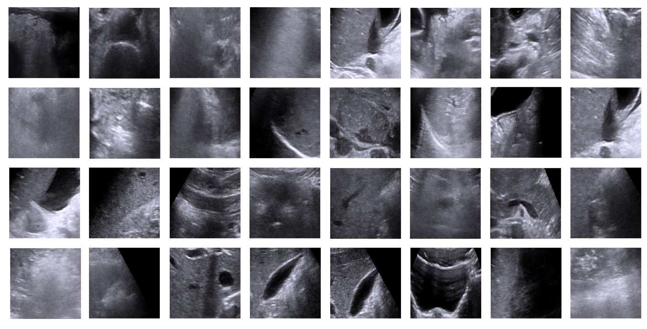
For training the Viola–Jones algorithm, 640 images (positive images: 320; negative images: 320) are used. The positive and negative images used in training the cascade classifier are shown in
Figure 8 and
Figure 9, respectively. The positive training dataset consists of kidneys with 270 normal, 30 cyst and 20 stone cases. The negative training dataset consists of 82 liver, 78 heart, 75 carotid and 85 spleen images. The region of interest for kidney differs from image to image. Therefore, in the training, all of the positive instances are rescaled to the expectation of width, the height of positive instances using nearest neighbor approach. The expectation for the region of interest is found to be 32 × 54 pixels.
Figure 8.
Some of the kidney images of the positive training dataset used in training the Viola–Jones algorithm.
Figure 8.
Some of the kidney images of the positive training dataset used in training the Viola–Jones algorithm.
Figure 9.
Some of the images of the negative training dataset used in training the Viola–Jones algorithm.
Figure 9.
Some of the images of the negative training dataset used in training the Viola–Jones algorithm.
The kidney detection algorithm is trained using a 20-stage cascade classifier with a 0.2 false alarm rate. For training each stage in the cascade classifier, positive and negative examples are considered with a 1:2 ratio. In training the object model for kidney, each stage uses at most 320 positive instances and 640 negative instances. Negative instances are generated automatically from the negative images. The number of features used in first five stages of the cascade classifier are 3, 5, 4, 5 and 6, respectively. A total of 92 features are selected from 586,000+ features. The kidney detection algorithm is realized using functions of the Viola–Jones algorithm available in OpenCV. The inbuilt functions in OpenCV take the false alarm rate and the number of cascade classifiers as the input parameters and generate a model with feature selection and threshold parameters for cascade classifiers.
MATLAB 2015a running on a desktop with an i7 processor, 16 GB RAM and a 2.8-GHz clock takes 17.25 min to train the cascade model for kidney detection. The model generated from MATLAB is compatible with OpenCV and is used to detect the kidney in real time on an ARM processor.
The number of features and the threshold for each cascade classifier are automatically detected by the Adaboost algorithm. The number of features and the threshold are selected based on the given false alarm rate. The true positives of the detector increase with the increase in false positives, as shown in
Table 1. The increase in false positives reduces the specificity and positive predictive value; ideally, these values should be equal to one. One hundred percent accuracy can be achieved with the cost of reducing the specificity and positive predictive value. An increase in parameters, like window enlargement in every step and displacement of the sliding window, slightly increases the detection speed at a cost of a slight decrease in accuracy. Detection accuracy heavily depends on false detections. A strong two-stage classifier with 100% detection accuracy can be constructed by keeping false alarms at more than 40%. The number of features selected for classification depends on the Adaboost algorithm. The detection time increased as the number of features used for classification increased. The displacement of the sliding window in detecting the kidney affected the accuracy of detection. The results presented here are for a one-pixel displacement. The detection time is improved with a two-pixel shift with slightly reduced accuracy.
Table 1.
Number of false detections vs. accuracy.
Table 1.
Number of false detections vs. accuracy.
| Number of False Positives (%) | Accuracy (%) |
|---|
| 13 | 83 |
| 20 | 91 |
| 25 | 93.5 |
| 30 | 98 |
| 35 | 100 |
| 40 | 100 |
The kidney detection algorithm is initialized with the following parameters: the window enlargement in every step is set to 1.1, and every time, the sliding window is shifted by one pixel. A 10-fold cross-validation scheme is employed to test the variability in the database. The 10-fold cross-validation is applied on the test set ten times with different partitions. Ten random seeds are generated, each of them separating the test set into 10 disjoint sets. Each subset is used for testing, while the other remaining nine sets are used in training. Each 10-fold cross-validation produces classification results for 320 kidney and 320 non-kidney images. Thus, a total instance of 3200 and 3200 kidney and non-kidney images is tested. The overall classification accuracy is averaged over ten rounds. The Viola–Jones algorithm performed with an overall accuracy of 92.6% in detecting kidney.
4. Experimental Setup and Results
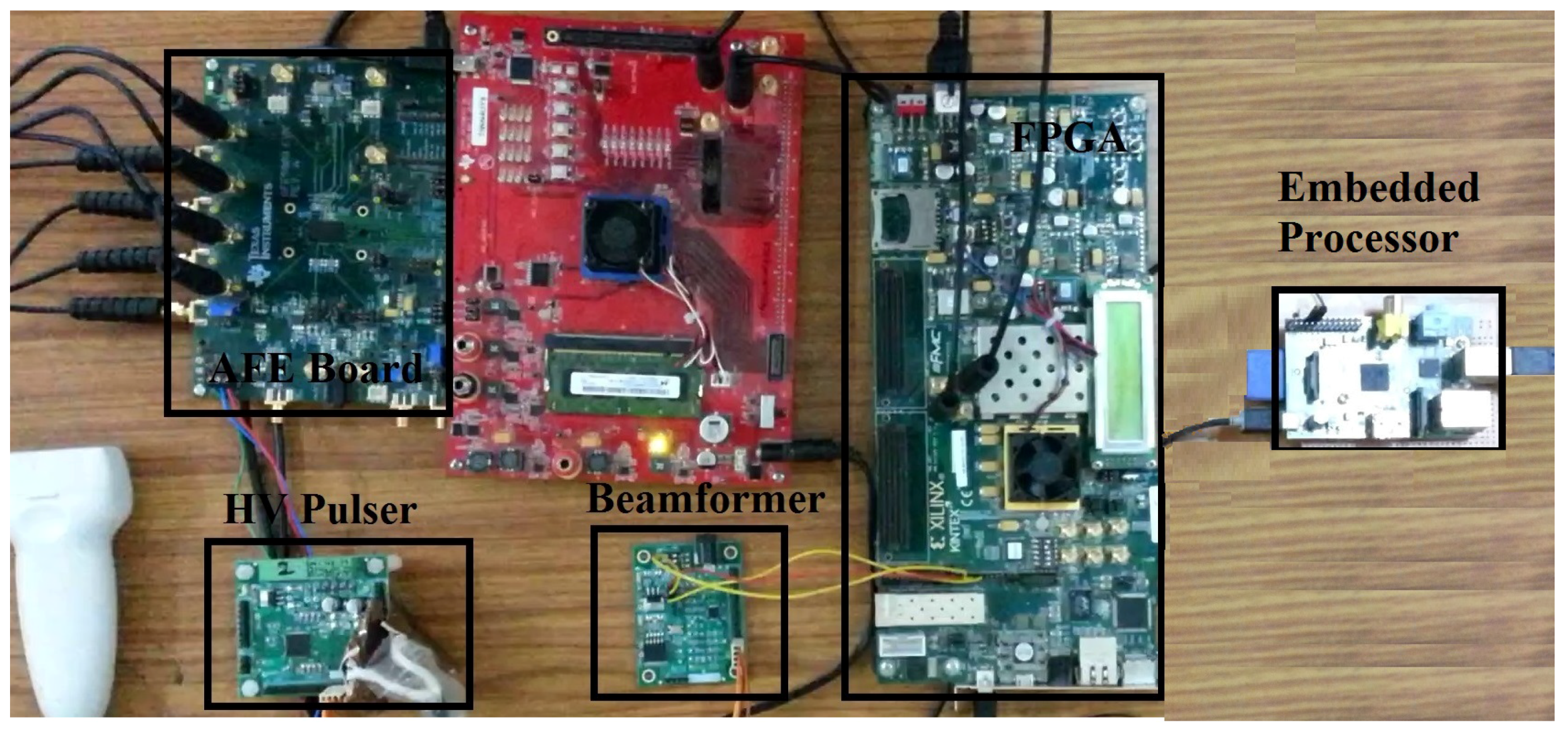
The prototype of the FPGA-based portable ultrasound scanning system is shown in
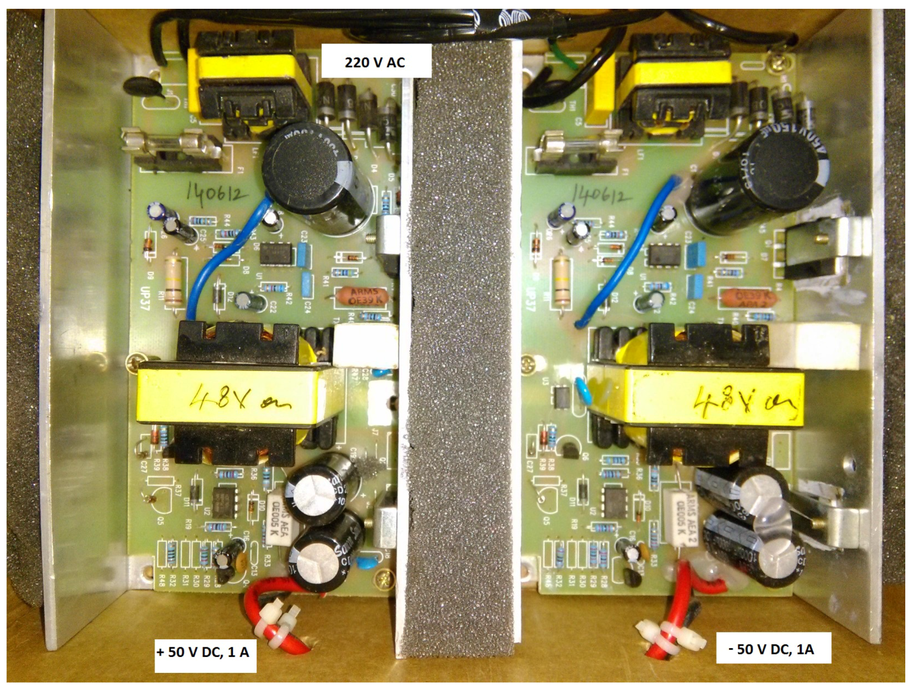
Figure 16. The transducer elements are excited with a voltage of ± 50 V with a 1-A current. A custom-made power supply is designed to generate the required voltage, as shown in
Figure 17. A 230-V, 50-Hz supply is given as the input to the power supply. A step down transformer is used to convert AC supply to ±50-V DC voltage with a 1-A current. These voltages are connected to the HV pulser for generating HV pulses to excite the transducer.
Figure 16.
Prototype of the proposed FPGA-based portable ultrasound scanning system.
Figure 16.
Prototype of the proposed FPGA-based portable ultrasound scanning system.
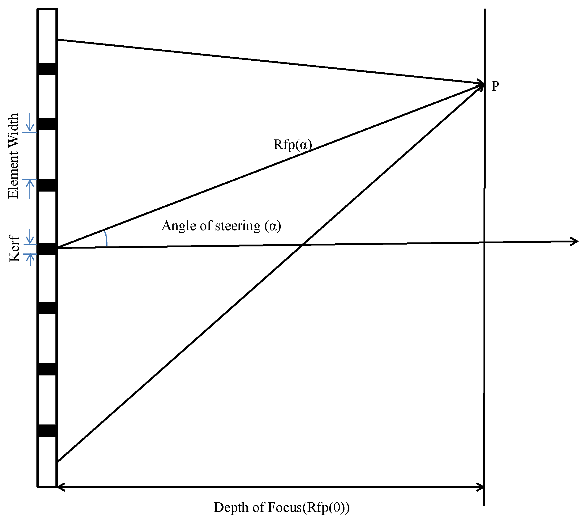
The performance of the proposed PUS system is evaluated by scanning a tissue-mimicking gelatin phantom. The specifications of the scanner used for scanning the phantom are shown in
Table 3. Out of 64 elements, eight transducer elements are active all of the time in transmitting ultrasound waves and receiving echoes from the tissue. The delay values of the channel are automatically updated depending on the receive focal zones.
Figure 17.
Power module designed for generating ±50 V DC.
Figure 17.
Power module designed for generating ±50 V DC.
Table 3.
Parameters used for scanning the gelatin phantom.
Table 3.
Parameters used for scanning the gelatin phantom.
| Specifications | Value |
|---|
| Transmit frequency | 5 MHz |
| Number of channels | 8 |
| Kerf of transducer | mm |
| Element width | mm |
| Depth of scan | 50 mm |
| Number of scanlines | 192 |
The performance of the proposed portable ultrasound system is evaluated by comparing to the commercially available platforms, like the PCI Extensions for Instrumentation (PXI) system and Biosono.
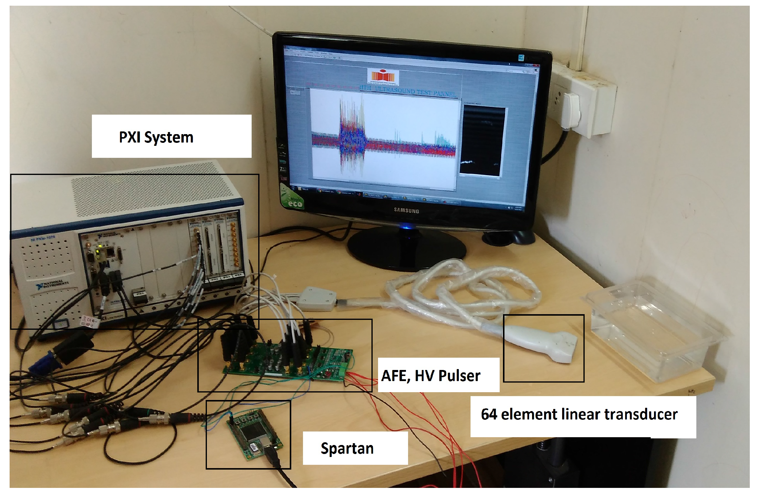
4.1. Ultrasound Scanning System Based on PCI Extensions for Instrumentation
National Instrument’s (NI) PXIe-1078 [
52] is a rugged PC-based platform for measurement and automation systems. It has two eight-channel high speed analog input modules. We have interfaced our data acquisition board to the PXI analog channels. Spartan-3 FPGA [
53] is used to establish synchronization between PXI and our data acquisition module.
Figure 18 shows the PXI platform hardware setup. The portable ultrasound board is provided with control pins in the FPGA to program the transmission parameters for the logic pulse driver. The FPGA generates a transmit control signal, which is used for synchronization of the PXI with the ultrasound front-end board. The PXI system uses LABVIEW 2013 software to acquire high speed ultrasound data and to reconstruct the ultrasound image. A linear array transducer with a center frequency of 5 MHz is used to scan the gelatin phantom.
Figure 18.
Ultrasound system based on the PCI Extensions for Instrumentation (PXI) platform.
Figure 18.
Ultrasound system based on the PCI Extensions for Instrumentation (PXI) platform.
4.2. Biosono Ultrasound Platform
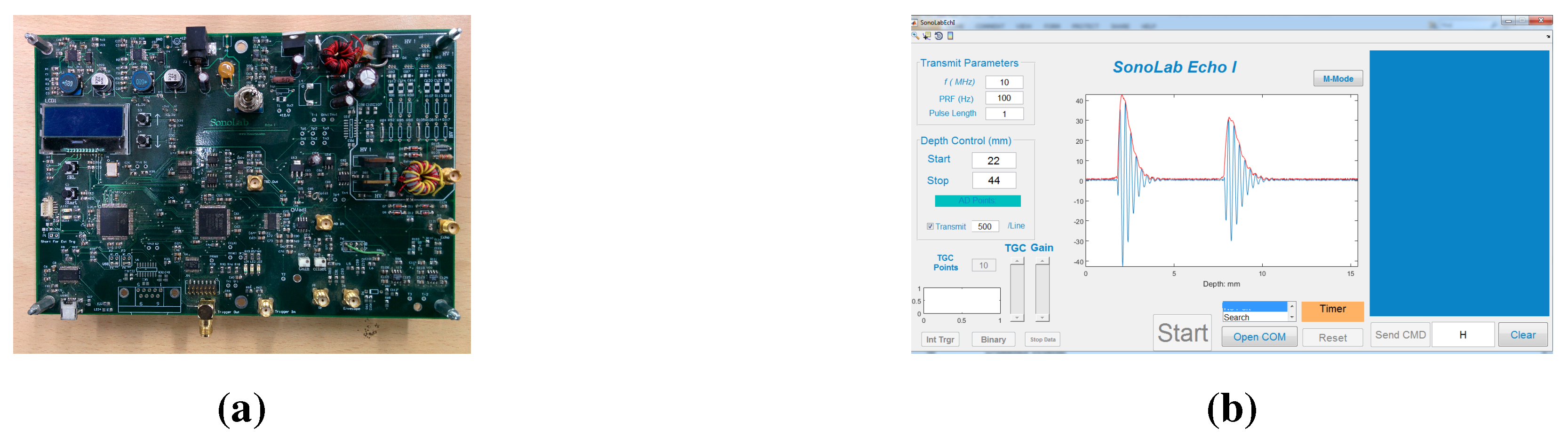
The proposed portable ultrasound data acquisition module is compared to the Biosono ultrasound platform.
Figure 19a shows the Biosono ultrasound board designed for A-mode and M-mode imaging applications [
54]. The echos are sampled and digitized at a rate of 100 MHz and streamed out through the serial port at 115,200 bps. The MATLAB GUI (
Figure 19b) is provided for viewing the real-time echo.
Figure 19.
Biosono ultrasound board. (a) Biosono board; (b) GUI for the Biosono board.
Figure 19.
Biosono ultrasound board. (a) Biosono board; (b) GUI for the Biosono board.
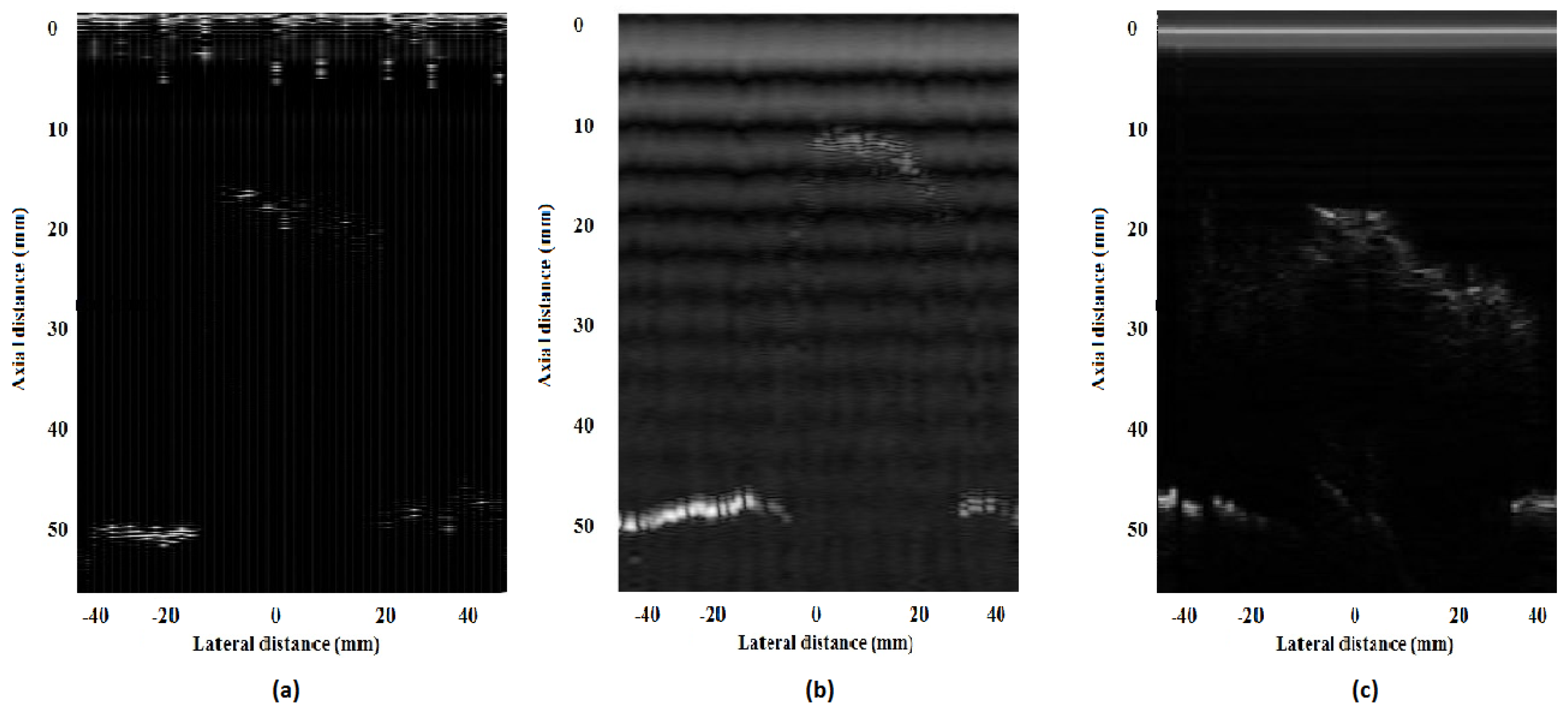
The visual comparison of the gelatin phantom image reconstructed from Biosono, NI and the proposed FPGA-based portable ultrasound scanning system is shown in
Figure 20. The geometrical shapes look similar in all of the images, validating the performance of the proposed FPGA-based portable ultrasound scanning system.
The resources utilized in the Kintex-7 FPGA for implementing the beamforming, mid-end and back-end algorithms are analyzed using the Xilinx ISE 14.4 synthesis tool, and this is summarized in
Table 4. The ultrasound signal processing algorithms use only 53% of the available LUT flip flops, so the remaining resources can be utilized for implementing other complex beamforming and image-processing algorithms.
Figure 20.
Image acquired and reconstructed from: (a) the Biosono platform; (b) the NIPXI platform; (c) the proposed FPGA-based portable ultrasound scanning system.
Figure 20.
Image acquired and reconstructed from: (a) the Biosono platform; (b) the NIPXI platform; (c) the proposed FPGA-based portable ultrasound scanning system.
Table 4.
Resources utilized in the Kintex-7 board for implementing the beamforming, mid-end and back-end processing algorithms.
Table 4.
Resources utilized in the Kintex-7 board for implementing the beamforming, mid-end and back-end processing algorithms.
| Resources Available | Resource Used | Percentage |
|---|
| Slice Logic Utilization | | |
| Number of slice registers (437,200) | 7351 | 1% |
| Number of slice LUTs (218,600) | 6086 | 2% |
| Number used as logic (218,600) | 5329 | 2% |
| Slice Logic Distribution | | |
| Number of LUT flip flop pairs used | 7,960 | |
| Number with an unused flip flop (7,960) | 1,867 | 23% |
| Number with an unused LUT (7,960) | 1874 | 23% |
| Number of fully-used LUT-FF pairs (7,960) | 4219 | 53% |
| Number of unique control sets | 382 | |
| IO Utilization | | |
| Number of IOs (250) | 60 | 24% |
| Specific Feature Utilization | | |
| Number of block RAM/FIFO (545) | 64 | 11% |
| Number of global clock buffers BUFG/BUFGCTRLs (32) | 16 | 18% |
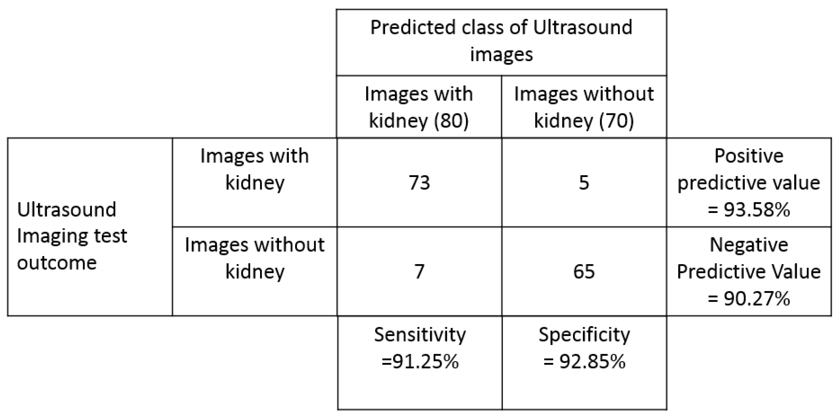
The performance of the automatic kidney detection algorithm is evaluated using the confusion matrix discussed in
Section 2.2. The confusion matrix of the proposed automatic kidney detection algorithm is shown in
Figure 21.
Figure 21.
Confusion matrix for the proposed automatic kidney detection algorithm.
Figure 21.
Confusion matrix for the proposed automatic kidney detection algorithm.
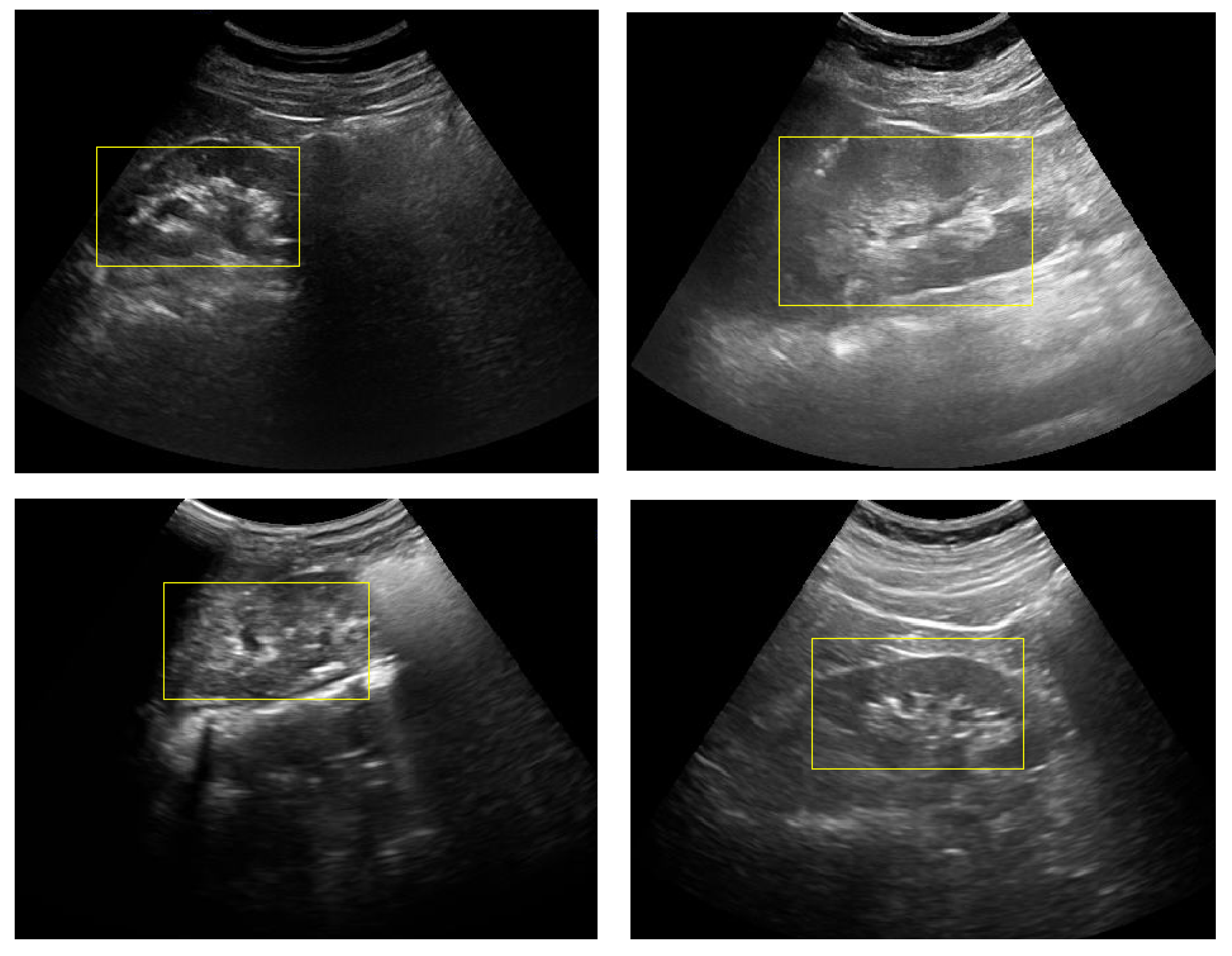
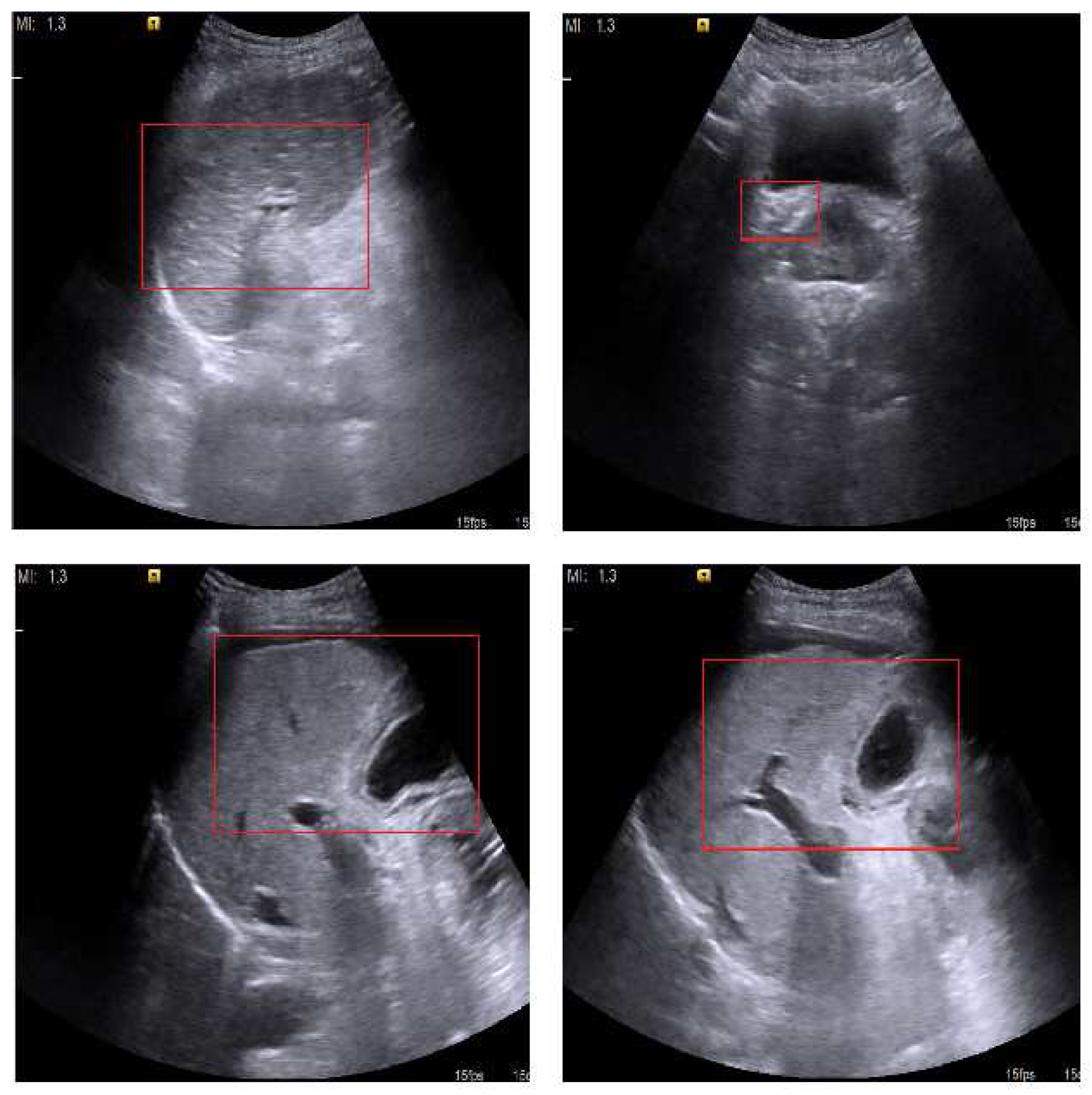
The kidney detection algorithm was tested on 80 kidney images (normal: 62; cyst: 10; stone: 8) and 70 non-kidney images (liver: 18; heart: 17; carotid: 15; spleen: 20). The kidney detection algorithm performed with an accuracy of 92% (138 out of 150), a sensitivity of 91.25%, a specificity of 92.85%, a positive predictive value of 93.58% and a negative predictive value of 90.27% in detecting the kidney in ultrasound images. False negatives (seven images) include two kidney images with cysts and one kidney image with stones. Multiple detections of kidney are an inherent property of the Viola–Jones algorithm, which is a result of detecting the organs at multiple scales, as shown in
Figure 22. Multiple windows with overlapping regions of interest are merged into a single window by averaging the coordinates of the window. The merging is allowed only if the kidneys have the minimum number of detections. Having a low threshold for multiple detections give rise to high false positives, and a high threshold leads to high false negatives. From observations, it is found that a threshold of 50 gives the maximum accuracy for detecting the kidney. The detection of kidney using the Viola–Jones algorithm is shown in
Figure 23. Some of the false positives that are detected in localizing kidney in the images are shown in
Figure 24.
Figure 22.
Multiple detections of kidney in ultrasound images.
Figure 22.
Multiple detections of kidney in ultrasound images.
Figure 23.
Automatic kidney detection.
Figure 23.
Automatic kidney detection.
Figure 24.
False positives detected in localizing the kidney.
Figure 24.
False positives detected in localizing the kidney.
The automatic kidney detection algorithm on Raspberry Pi-2 (900 MHz, 1 GB RAM) takes 60 ms to detect the presence of kidney in a 480 × 640 resolution frame. The kidney detection algorithm is used as an add-on feature in the Raspberry Pi board. By enabling the kidney detection option, the system directly applies the algorithm on the incoming frame, which is stored in the SDRAM.
For evaluating the kidney detection algorithm in real time, an ultrasound video is acquired from 10 patients using the Siemens S1000 through Ultrasonix 500RP [
55]. The scanned kidney videos have a frame rate of 15 fps, and this is transferred to the SDRAM of the Raspberry Pi processor. The kidney detection algorithm installed on the Raspberry Pi processor is successfully able to detect the kidney in live streaming video.
Implementing the Viola–Jones algorithm on an FPGA requires 11,505 slice registers, 7,872 slice flip flops, 20,901 four-input LUTs, 44 block RAM (BRAM) and one global clock (GCLK) buffer [
56]. Optimized algorithms have been proposed for fast real-time implementation of the Viola–Jones algorithm to detect faces in video having frame rates greater than 100. The Viola–Jones algorithm is effectively implemented on various computing platforms, like FPGAs, DSPs, GPUs, mobile platforms,
etc. [
56,
57,
58,
59]. The same computing platforms are also used for realizing PUS systems, so the Viola–Jones algorithm can be implemented on these platforms for real-time detection of kidney. From
Table 4, the Kintex-7 has enough resources to implement the Viola–Jones algorithm. Implementing the kidney detection algorithm on an FPGA platform will reduce the load on the ARM processor, which can be used for other tasks, like real-time recording, compression, data transferring,
etc.


