FTIR-Based Microplastic Classification: A Comprehensive Study on Normalization and ML Techniques

Abstract

This study examines the potential of machine learning (ML) and deep learning (DL) techniques for classifying microplastics using Fourier-transform infrared (FTIR) spectroscopy. Six commonly used industrial plastics (PET, HDPE, PVC, LDPE, PP, and PS) were analyzed. A significant contribution of this research is the use of broader and more varied spectral ranges than those typically reported in the state of the art. Furthermore, the impact of different normalization techniques (Min-Max, Max-Abs, Sum of Squares, and Z-Score) on classification accuracy was evaluated. The study assessed the performance of ML algorithms, such as k-nearest neighbors (k-NN), support vector machines (SVM), naive Bayes (NB), random forest (RF), and artificial neural networks architectures (including convolutional neural networks (CNNs) and multilayer perceptrons (MLPs)). Models were trained and validated using the FTIR-PLASTIC-c4 dataset with a 10-fold cross-validation approach to ensure robustness. The results showed that Z-score normalization significantly improved stability and generalization across most models, with CNN, MLP, and RF achieving near-perfect values in accuracy, precision, recall, and F1-score. In contrast, the sum of squares normalization was less effective, particularly for CNNs, due to its sensitivity to scale and data distribution. Notably, naive Bayes consistently underperformed because of its limitations in analyzing complex spectral data. The findings highlight the effectiveness of FTIR spectra with broad and variable ranges for the automated classification of microplastics using ML techniques, along with appropriate normalization methods.

1. Introduction

Plastic pollution, primarily a consequence of human activities, extends its detrimental effects from terrestrial areas to the most remote oceans [1]. Over the past decades, the consumption of plastic products has grown exponentially due to their indispensability in modern society [2]. Their unique properties—durability, flexibility, and resilience—make them ideal for construction, healthcare, electronics, and packaging applications, among other sectors [3]. Common plastics such as polyethylene terephthalate (PET), high-density polyethylene (HDPE), polyvinyl chloride (PVC), low-density polyethylene (LDPE), polypropylene (PP), and polystyrene (PS) dominate modern usage. Yet, only a tiny fraction is effectively recycled [4].

The exposure of plastic waste to solar radiation, wind, and mechanical forces promotes its fragmentation into smaller particles, facilitating its dispersion and persistence in the environment [5]. This process transforms macroplastics (MAP) into microplastics (MP) and, subsequently, nanoplastics (NP). The environmental challenge posed by plastic waste is exacerbated by its resistance to natural degradation, persisting for centuries or even millennia. Furthermore, the smaller size of MPs and NPs increases the likelihood of their penetration into living organisms [6].

Microplastics, a term introduced by Thompson [7], are persistent environmental contaminants. Significant amounts have been detected in oceans, sediments, and aquatic organisms, particularly in the intestines and stomachs of certain fish [8]. The accumulation of MPs in the organs of these organisms can lead to inflammation, intestinal obstruction, and toxicity, raising concerns about human health risks due to seafood consumption [9]. This reveals the urgency of addressing MP pollution. Moreover, MPs can carry toxic chemicals, including pesticides and heavy metals, and serve as reservoirs for pathogenic microorganisms [10]. The persistence and accumulation of MPs in the environment implies critical challenges to environmental and human health, which makes imperative comprehensive plastic waste management and innovative remediation technologies [11].

Traditional MP detection methods in freshwater and seawater involve sieving or density separation techniques [12]. MPs are then quantified by size and color, followed by compositional analysis [13]. Spectroscopic techniques such as Fourier-transform infrared (FTIR) and Raman are widely used for structural analysis of MPs. However, Raman spectroscopy is prone to interference from pigments and surrounding materials. In contrast, FTIR spectroscopy often produces weak or overlapping vibrational bands due to the small size of MPs [14].

Manual methods for MP classification remain labor-intensive, time-consuming, and error-prone, as they involve microscopic examination for identification and characterization [15]. To overcome these limitations, there is an urgent need for faster, more accurate, and accessible monitoring tools capable of mitigating the shortcomings of conventional methods [16]. Spectroscopic techniques, particularly FTIR, offer a promising solution. FTIR is a non-destructive method that identifies MPs by detecting characteristic spectral peaks associated with various polymers, making it a valuable tool for advancing automated MP classification [17]. In recent years, artificial intelligence (AI) has emerged as a transformative tool for automating labor-intensive processes requiring specialized knowledge [18]. Studies combining FTIR spectroscopy with machine learning (ML) algorithms have demonstrated the potential to reduce errors and processing times through multivariate analysis [19].

ML algorithms such as decision trees (DT), random forests (RF), support vector machines (SVM), and k-nearest neighbors (kNN) [20], including DL techniques like artificial neural networks (ANNs), have been applied to spectral data across various scientific disciplines. Recently, deep learning methods, mainly convolutional neural networks (CNNs) and multilayer perceptrons (MLPs), have shown significant potential in infrared spectral data analysis, enhancing prediction accuracy and noise tolerance.

In this context, this study aims to compare various ML algorithms for MP classification using a publicly available FTIR spectra database (FTIR Plastic-c4). This database comprises FTIR spectra of six widely used polymers (PET, HDPE, PVC, LDPE, PP, and PS) and MP fractions of 5 mm. The objective is to explore the effectiveness of combining plastic material characterization through FTIR spectroscopy with ML classification techniques for identifying MPs extracted from water samples. The results demonstrate the efficacy of this approach in classifying MPs smaller than 5 mm.

2. Related Works

Automated waste classification is important for enhancing the efficiency of recycling processes. Several studies have explored using convolutional neural networks (CNNs) for this purpose. For instance, Altikat et al. [21] proposed a CNN to classify waste into categories such as paper, glass, plastic, and organic matter, achieving an accuracy between 76.7% and 83.0%. Their work focused on improving plastic recycling within mixed urban waste, emphasizing the need for systems capable of identifying plastic subcategories to optimize recycling and recovery processes. Similarly, Zhang et al. [22] implemented a transfer learning scheme to reduce training times and used pre-existing knowledge in waste classification. Using the NWNU-TRASH dataset, their model classified samples of paper, plastic, glass, metal, and fabric, achieving an accuracy of 82.8%. The authors demonstrated the importance of distinguishing between different types of plastics in mixed waste streams to improve segregation.

For polymer identification, Bobulski et al. [23] proposed a 15-layer CNN architecture to identify common household plastics such as HDPE, PET, PP, and PS from RGB (red-gray-blue scale) images. Although they achieved a high training accuracy of 99%, the testing accuracy dropped to 74%. It resembles the potential and challenges of deep CNN architectures in capturing variability within plastic waste classes.

Moreover, image-based classification becomes insufficient when identifying plastics at the micro and nano levels. Specialized techniques, such as hyperspectral imaging, for example, are required. Singh et al. [24] used a Specim FX17 NIR (near infra-red) hyperspectral camera to capture frequency bands in the 900–1700 nm range and trained a gradient boosting algorithm to identify eight types of plastics. They achieved an overall accuracy of 79%, which increased to 90% when excluding black plastics, demonstrating the potential of hyperspectral spectroscopy for colored plastic classification.

Another promising approach is mid-infrared (MIR) spectroscopy, particularly Fourier-transform infrared spectroscopy (FTIR). For instance, Zinchik et al. [25] proposed PlasticNet, a CNN for classifying binary and ternary mixtures of microplastic waste (MPW) based on IR spectra. Their model achieved 100% accuracy with a prediction speed of up to 8200 Hz, outperforming current MIR spectrometers. This approach combines MIR spectra and CNNs to offer a cost-effective, high-efficiency tool, making it a viable option for real-time plastic analysis and classification. Conversely, Jeon et al. [26] focused on partial least squares discriminant analysis (PLS-DA) for classifying plastics such as HDPE, LDPE, PP, PS, and PVC from FTIR spectra. Their methodology included spectral normalization and dimensionality reduction using principal component analysis (PCA), achieving 91% accuracy in distinguishing between HDPE and LDPE and showing sensitivity and specificity exceeding 94% across all classes.

FTIR spectroscopy in its attenuated total reflectance (ATR) mode has emerged as an effective method for identifying microplastics [27]. Techniques such as SVM, random forest, kNN, LDA, CNN, and MLP have been employed to classify ATR-FTIR spectra, achieving accuracies above 92% in experiments using various datasets [28]. However, in these studies, the datasets used are either private or limited to specific spectral ranges, and the IR spectra exhibit low variability within each sample.

Thus, the primary contribution of this study is the classification of microplastics across broader spectral ranges using a public dataset, enabling direct comparison with other proposals. Our research employs Fourier-transform infrared spectroscopy in the 4000–400 cm⁻¹ range to analyze the spectra of materials (PET, HDPE, PVC, LDPE, PP, and PS), which correspond to the most common industrial plastics.

3. Theoretical Foundations

The classification of microplastics addresses an increasingly significant environmental problem, which presents notable challenges due to the diversity of plastic types, variations in size, and the complexity of sample extraction and separation. Current approaches seek to resolve such issues through applications or devices using artificial intelligence (AI), with computers as the primary tool in these processes [29]. However, the inherent difficulties in handling and analyzing microplastic samples, mainly due to their size, necessitate adopting specialized techniques and methodologies. In this context, a subfield of AI such as machine learning (ML), which includes deep learning (DL) [30], offers promising solutions by providing accuracy and speed for microplastic classification. ML and DL enable advanced algorithms to process data, identify patterns, propose optimized solutions, and ensure high precision and adaptability across various applications. Such capabilities are critical for achieving effective and reliable microplastic classification [31].

3.1. Machine Learning

Machine learning is a branch of artificial intelligence that enables algorithms to learn and improve automatically from experience without explicit programming [32]. This approach focuses on studying and training algorithms to solve complex and adaptive problems, broadening their applicability in tasks such as recognition and classification across various domains [33]. The learning process relies on datasets organized into training, testing, and, in some cases, validation sets, allowing models to generalize conclusions tailored to the specific characteristics of each problem [34]. Traditional ML algorithms commonly include k-nearest neighbors (kNN), support vector machines (SVM), Bayesian networks, and random forest.

• k-Nearest Neighbors (kNN):
  This supervised classification method is based on proximity, assigning a class to a new datapoint based on the classes of its closest neighbors in the feature space [35]. The simplicity of kNN lies in its structure, as it does not require a pre-trained model or assumptions about data distribution. The model’s accuracy heavily depends on the choice of “k” (number of neighbors); a low value of k may result in sensitivity to noise, while a high value may overly smooth class boundaries [36]. kNN is suitable for classification tasks in areas such as image recognition, recommendation systems, and pattern recognition where classes are well-defined.
• Support Vector Machines (SVM):
  The SVM is a supervised classification algorithm designed to find the optimal hyperplane that maximizes the margin of separation between classes in the feature space [37]. This approach minimizes the probability of misclassification on test data. For non-linearly separable data, kernel functions are employed to project the data into higher-dimensional spaces, facilitating separation [38]. SVM has proven effective in tasks like text classification, pattern recognition, and image analysis, particularly where clear boundaries between classes exist.
• Bayesian Networks:
  Bayesian networks are probabilistic graphical models that represent causal relationships among variables and utilize Bayes’ theorem to update event probabilities based on available evidence [39]. These models integrate prior knowledge and represent conditional dependencies between variables, making them suitable for problems involving interdependent variables [40]. They have demonstrated efficacy in decision-making under uncertainty and in contexts with prior knowledge, such as medical diagnosis, financial risk assessment, and recommendation systems.
• Random Forest:
  Random forest is an ensemble learning algorithm that combines multiple decision trees to enhance prediction accuracy and reduce overfitting risk [41]. The algorithm constructs several independent decision trees using different random samples of the dataset and aggregates their outputs through methods such as majority voting for classification or averaging for regression. Its ability to handle redundant or irrelevant features and mitigate overfitting makes random forest a robust tool for complex problems with high-dimensional data. It is commonly applied in classification tasks such as image analysis, bioinformatics, and fraud detection [42].

On the other hand, deep learning (DL) is an advanced field of ML that uses artificial neural networks (ANNs) with several hidden layers to imitate the human brain’s learning process [43]. Using computational tools, DL replicates numerous neural connections, similar to biological synapses, to identify and extract features from input data, forming complex representations through successive transformations. This process is refined with mathematical and statistical methods, improving the models’ accuracy and efficiency [44].

Artificial neural networks, the fundamental building blocks of DL, have applications in areas like image recognition, speech processing, and text analysis. Made up of hierarchical layers, ANNs capture more complex features as each layer processes the information from the previous one. During training, the weights that connect the neurons are optimized, enabling the ANN to learn and generalize patterns. However, a significant drawback is overfitting, which happens when the model adapts excessively to the training data, hindering its performance on new data [45].

• Multilayer Perceptron (MLP):
  The multilayer perceptron is a type of artificial neural network that includes at least one hidden layer. In the context of deep learning, it incorporates multiple hidden layers between the input and output layers [46]. In MLPs, each neuron is connected to the neurons in the subsequent layer through synaptic weights, which are adjusted during training via the backpropagation method. This optimization process enables the MLP to capture complex, non-linear patterns in data, making it suitable for classification and regression tasks [47]. Its versatility and capacity to approximate any continuous function have made it popular for applications such as time series prediction, speech recognition, and image classification.
• Convolutional Neural Networks (CNN):
  Convolutional neural networks are specialized neural networks designed for processing grid-like data structures, such as images [48]. CNNs consist of convolutional layers that apply filters to extract spatial features and visual patterns, as well as pooling layers that reduce dimensionality in the representations obtained during convolution. This architecture enables CNNs to detect hierarchical patterns in data, making them highly effective for tasks such as image classification, semantic segmentation, and video analysis [49]. CNNs have transformed the field of deep learning, demonstrating exceptional performance in applications like facial recognition, medical diagnosis, and real-time object detection.

3.2. Normalization Techniques

Normalization is a fundamental step in data preprocessing. It ensures that the heterogeneity of datasets does not hinder the performance of ML models. Data used in these models often originate from diverse sources and present varying scales, distributions, and units of measurement. Without normalization, disparities in data magnitudes can lead to biased models that fail to generalize effectively.

Normalization addresses these challenges and improves model performance by rescaling or transforming data to a uniform scale. For example, optimization algorithms like gradient descent, which are commonly used in DL, converge faster and more reliably when input features are normalized. Moreover, some algorithms, such as support vector machines or neural networks, are sensitive to variations in feature scaling; normalization ensures that these models learn equally from all features instead of being dominated by those with larger magnitudes.

In this study, spectroscopic data are particularly susceptible to variability due to their inherent complexity, which includes noise, changes in measurement conditions, and sample heterogeneity. Proper normalization helps mitigate these factors, reducing redundancy, enhancing data integrity, and allowing for the extraction of meaningful patterns. The normalization techniques used in this research are as follows [50]:

• Min-Max Normalization:
  This technique scales data to fit within a specific range, typically [$0,1$]. This is especially useful for algorithms sensitive to the range of input data, such as neural networks that use activation functions like sigmoid or tanh, which operate best with inputs in a constrained range (Equation (1)).

  $$x^{\prime }={\displaystyle \frac{x-min\left(x\right)}{max\left(x\right)-min\left(x\right)}},$$

  (1)

  where x represents a data point, $min\left(x\right)$ is the minimum value, and $max\left(x\right)$ is the maximum value in the dataset.
• Max-Absolute Normalization:
  This method divides each data point by the maximum absolute value in the dataset, adjusting values to lie within the range [$-1,1$]. This technique is particularly beneficial when datasets contain negative values and need to maintain their relative magnitude relationships (Equation (2)).

  $$x^{\prime }={\displaystyle \frac{x}{max\left(\right|x\left|\right)}},$$

  (2)
  Here, x is a data point, and $\max \left(\right|x\left|\right)$ represents the maximum absolute value in the dataset.
• Sum of Squares:
  Although not a direct normalization technique, this concept is fundamental in statistical model fitting, such as ANOVA and linear regression. In spectral data analysis, it addresses inherent variabilities like noise, sample variations, and light dispersion. The sum of squares quantifies variability across sample groups for each polymer, aiding in identifying significant differences between spectra (Equation (3)).

  $$x^{\prime }={\displaystyle \frac{x}{\sqrt{{\sum }_{i=1}^n{x}_i^2}}},$$

  (3)

  where x is a data point, and $\sum x_i^2$ denotes the sum of squared data points.
• Z-score Standardization:
  Z-score standardization measures the relative position of an observation within a dataset in terms of standard deviations from the mean. This technique is critical when comparing datasets with different distributions or identifying outliers. Moreover, it is particularly suited for algorithms assuming normally distributed input data, such as principal component analysis (PCA) (Equation (4)).

  $$Z={\displaystyle \frac{x-\mu }{\sigma }},$$

  (4)
  Here, x is a data point, $\mu$ is the dataset mean, and $\sigma$ is the standard deviation.

By ensuring that all features contribute proportionally to the learning process, normalization improves the accuracy and reliability of ML models while minimizing computational inefficiency. Furthermore, in domains like spectroscopy, where even small data variations can significantly impact outcomes, normalization helps isolate the essential signal from noise, allowing the models to extract valuable insights and produce consistent, reproducible results.

3.3. Classifier Performance

Evaluating the performance of classifiers in multi-class classification problems requires a comprehensive analysis of diverse metrics, such as accuracy, precision, recall, and F1-score. Collectively, these metrics provide a nuanced understanding of model effectiveness, balancing its strengths and potential limitations.

Among these, the macro F1-score is particularly valuable because it calculates the harmonic mean of precision and recall for each class and then averages these values. This approach ensures a balanced evaluation across all classes, even in situations with class imbalances. Although the FTIR-PLASTIC-c4 dataset does not show class imbalance, the F1-score remains a strong indicator for evaluating overall performance, as it offers insight into the trade-offs between precision and recall across all classes.

The combined analysis of accuracy, precision, recall, and F1-score provides a detailed perspective on model performance by assessing its effectiveness, computational complexity, and generalization ability. This is particularly important in multi-class classification tasks, where subtle variations between classes can significantly affect the model’s utility in real-world applications [51].

In multi-class classification problems, where more than two classes exist, metrics such as precision, recall, accuracy, and F1-score are adapted using the “one-vs-rest” technique. This approach treats each class as a positive class while considering all other classes as negative, effectively transforming the multi-class problem into multiple binary classification problems, where each instance of a class can be categorized in one of the following:

• True positive (TP): number of instances that are positive and correctly predicted as positive by the model;
• False negative (FN): number of instances that are positive but incorrectly predicted as negative by the model;
• True negative (TN): number of instances that are negative and correctly predicted as negative by the model;
• False positive (FP): number of instances that are negative but incorrectly predicted as positive by the model.

Then, the specific metrics used in this approach to assess the classifier performance are defined as follows [52]:

• Accuracy:
  Indicates the overall classification performance of the model on the test dataset and is calculated as by Equation (5).

  $$\mathrm{Accuracy}={\displaystyle \frac{TP+TN}{TP+TN+FP+FN}}$$

  (5)
• Recall:
  Reflects the model’s ability to correctly identify positive cases as a percentage of the total actual positive cases (Equation (6)).

  $$\mathrm{Recall}={\displaystyle \frac{TP}{TP+FN}}$$

  (6)
• Precision:
  Represents the proportion of predicted positive cases that are actually positive (Equation (7)).

  $$\mathrm{Precision}={\displaystyle \frac{TP}{TP+FP}}$$

  (7)
• F1-score:
  Provides a comprehensive evaluation of classification model performance by calculating the harmonic mean of precision and recall (Equation (8)).

  $$\mathrm{F}1\text{-}\mathrm{score}={\displaystyle \frac{2·TP}{2·TP+FP+FN}}$$

  (8)

The selection of these performance metrics is driven by their complementary roles in evaluating the classifier’s effectiveness. Accuracy offers a broad overview of the model’s success rate, while precision and recall examine its ability to identify positive instances and minimize false positives, respectively, accurately. The F1-score harmonizes these two metrics, making it essential to assess models in situations where false positives and negatives have significant consequences. This strategy ensures that the models developed for the FTIR-PLASTIC-c4 dataset classification tasks are accurate and generalizable across different data distributions.

Finally, after computing metrics for each individual class, aggregation methods such as micro-average, macro-average, or weighted average are employed. The choice of aggregation method depends on the analysis objectives and the class distribution within the dataset:

• Micro-average: weighs each instance equally, suitable for datasets with balanced or unbalanced class distributions;
• Macro-average: averages the metrics for all classes equally, regardless of the class size, providing a balanced view;
• Weighted average: accounts for class frequency, emphasizing the contribution of larger classes.

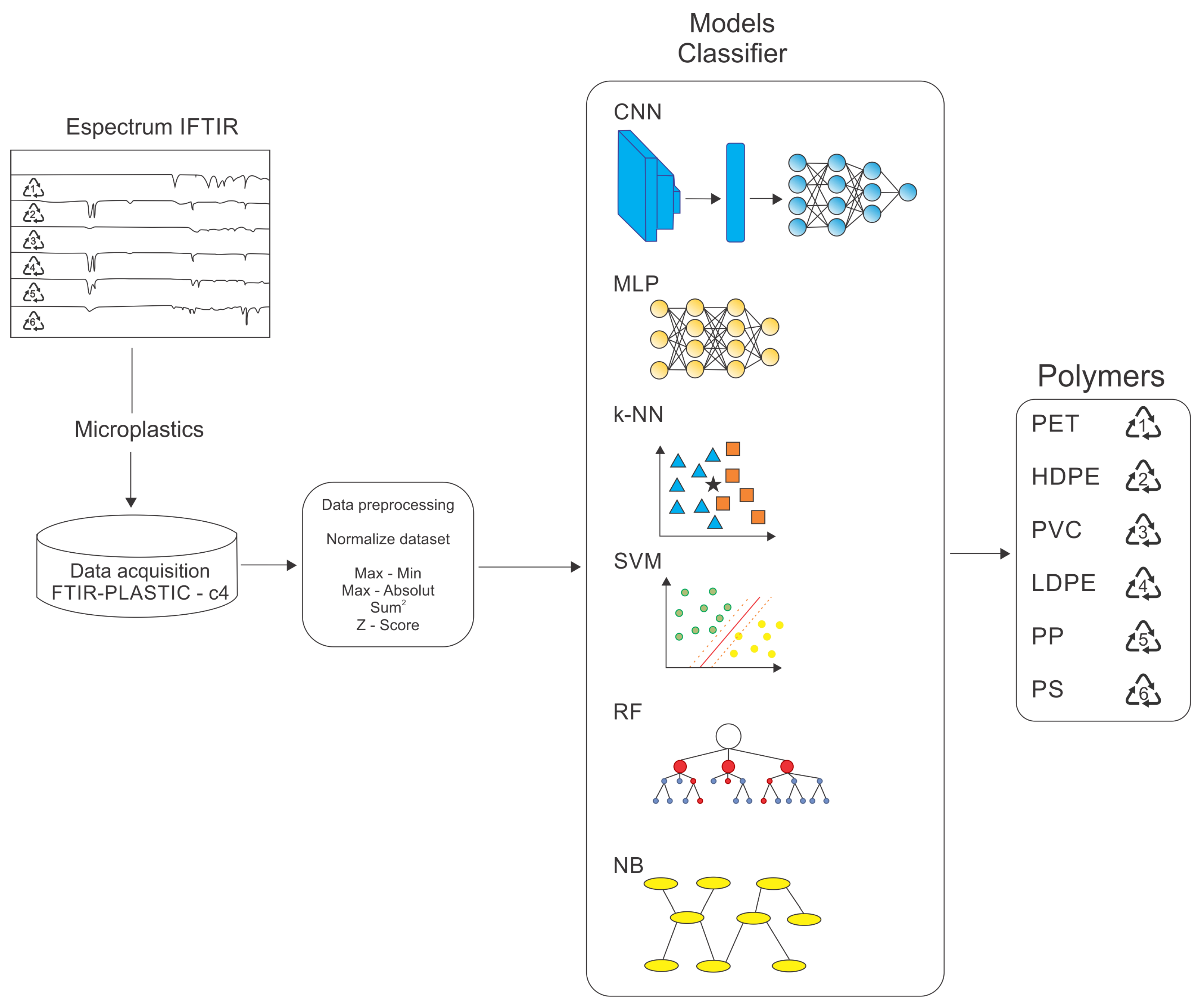
These averaging techniques ensure that the selected performance metrics align with the specific goals of the study, such as prioritizing underrepresented classes or achieving balanced performance across all classes.

4. Methods

This section describes the methodology for classifying microplastics using FTIR spectroscopic data through machine learning. The inherent complexity of microplastic classification stems from significant variability in chemical composition, particle morphology, and size. This variability leads to high-dimensional data that necessitate advanced analytical methods to extract meaningful patterns and insights.

ML (and its recent DL subset) techniques are widely recognized for their ability to model complex, non-linear relationships in intricate datasets. Their application to FTIR spectroscopic data establishes a robust framework for tackling the challenges of microplastic classification, delivering superior performance in pattern recognition and classification tasks across various scientific domains. The methodology, summarized in Figure 1, comprises the following key stages:

• Dataset acquisition: preparing and curating the FTIR-PLASTIC-c4 dataset;
• Data preprocessing: implementation of data cleaning, normalization, and transformation techniques to enhance data quality and ensure compatibility with the selected models;
• Choosing classifier models: identifying the most appropriate algorithms and architectures designed for the classification task;
• Training and testing: ML (or classifier) models involve the iterative optimization of model hyperparameters and validation with suitable evaluation protocols;
• Performance evaluation of classification models: a comprehensive analysis of performance metrics to assess the effectiveness, robustness, and generalization capability of the models.

4.1. Dataset

The dataset utilized for this study is the publicly available FTIR-PLASTIC-c4 dataset [53], selected for its significance in microplastic analysis. This dataset consists of 3000 FTIR spectra, evenly distributed among six polymer types (500 spectra per polymer).

Microplastics are generally defined as plastic particles within the size range of 1 μm to 0.5 cm, resulting from environmental fragmentation due to wind, solar radiation, and mechanical forces [54]. The FTIR-Plastic-c4 dataset used in this study was specifically designed for microplastic classification. This dataset contains FTIR spectra of plastic fragments ranging from 2 mm to 5 mm, which are representative of microplastics commonly found in aquatic environments. The choice of this size range was based on prior experimental findings indicating that microplastics in water typically fall between 0.131 mm and 4.098 mm. While larger particles produce strong and well-defined FTIR signals, smaller microplastics tend to exhibit weak vibrational bands, shoulder peaks, or secondary vibrations, making their spectral characterization more challenging. To mitigate this limitation, the spectral reference library utilized larger microplastic fractions (5 mm), allowing for the accurate identification of smaller particles (0.1 mm) based on their characteristic spectral features.

The concentration of microplastics in a sample can influence FTIR spectral intensity, especially in transmission and ATR-FTIR measurements, since higher concentrations lead to increased absorbance. However, peak positions remain unchanged, allowing for reliable classification. Moreover, all spectra in the dataset were collected under standardized measurement conditions to ensure consistency and minimize concentration-related spectral distortions.

It is important to note that while our approach is effective for identifying microplastics down to 0.1 mm, much smaller particles (1 μm) require alternative characterization techniques, such as scanning electron microscopy (SEM) or Raman spectroscopy, due to the limitations of FTIR spectroscopy at that scale. Nevertheless, the spectral data provided in this study are a good reference for microplastic identification in environmental samples.

Each spectrum in the FTIR-PLASTIC-c4 dataset is represented by 3751 features corresponding to spectral data within the range of 4000 to 400 cm⁻¹, as detailed in

Table 1. FTIR-PLASTIC-c4 datasets used to build the models presented in this work.

Dataset	Size (Samples)	Range (cm−1)	International Number (SPI)	Feature Data
PET	500	4000–400	1	3751
HDPE	500	4000–400	2	3751
PVC	500	4000–400	3	3751
LDPE	500	4000–400	4	3751
PP	500	4000–400	5	3751
PS	500	4000–400	6	3751

. Data were gathered using Fourier-transform infrared (FTIR) spectroscopy under the following conditions: 32 scans and two spectral resolutions of 8 cm⁻¹ and 4 cm⁻¹. Each spectrum was encoded into a scaled vector format, facilitating efficient model training, validation, and testing.

The dataset is publicly accessible through the ZENODO repository. For direct access, the database can be downloaded from https://zenodo.org/records/10736650. The repository also provides detailed information on the instrumentation and sample preparation protocols, highlighting key spectral characteristics like vibrational peaks that are critical for polymer identification. For this research, we accessed at this repository on 1 October of 2024.

To enhance the effectiveness of ML models, the percentage transmittance field in the FTIR-PLASTIC-c4 dataset was normalized using four different normalization techniques (see Section 3.2). This step was essential for evaluating the impact of each normalization method on the scaled data distribution. The analysis aided in identifying the most suitable normalization strategy for maintaining the spectral characteristics critical for polymer identification.

In the FTIR-PLASTIC-c4 dataset, the transmittance field captures material-specific properties, including vibrational bands and peaks. These peaks act as unique spectral patterns that enable the accurate identification of each polymer type. Proper normalization ensured that these key features were preserved during data preprocessing, thus maintaining the integrity of the spectral information used for model training.

4.2. Set-Up Parameters for the Studied Machine Learning Models

For this study, we utilized traditional classifiers like k-nearest neighbors (k-NN), support vector machine (SVM), naive Bayes (NB), and random forest (RF), and popular DL architectures as convolutional neural networks (CNN) and multilayer perceptrons (MLP). These models have been previously investigated in other research focused on microplastic classification. Their inclusion in this work allows for benchmarking our results against earlier studies and positions our methodology within the broader state-of-the-art framework in this field.

The ML models were developed and assessed using the 10-fold cross-validation technique, which divides the dataset into 10 random subsets for each microplastic type. To improve the robustness of the results, each algorithm was run 15 times, allowing for a reliable evaluation of model performance. The experimental results presented in this study reflect the average values obtained from these 15 runs across the 10 partitions created during the cross-validation process.

The hyperparameters were determined through a trial-and-error process. Each training-fold_i obtained from 10-fold cross-validation was randomly split into 80% (new training set, TD_new) and 20% (validation set, V), following the condition: training-fold_i = {TD_new$\cup V$}, {TD_new$\cap V\}=\varnothing$, for $i=1,2,\dots ,10$.

TD_new and V subsets were used to train and validate different hyperparameter configurations for each ML model, selecting those that maximized accuracy on V (see Section 3.3). Once the optimal hyperparameters were identified, the models were retrained using the full training-fold_i, and their final evaluation was conducted using the corresponding test-fold_i, which remained unseen during the hyperparameter tuning process. The best hyperparameters obtained for k-NN, SVM, and RF models are detailed below:

• k-NN: Seven neighbors were used for classification. The distance between neighbors was measured using the Euclidean metric, and uniform weights were assigned to all neighbors to ensure equal contribution.
• SVM: A cost parameter (C) of 1.00 was selected to control misclassification penalties. The RBF (radial basis function) kernel was used to capture non-linear similarities. Convergence criteria included a numerical tolerance of 0.0001 and an iteration limit of 500.
• Random Forest: The model utilized seven trees. In the growth control configuration, subsets with fewer than five samples were not further split. In this sense, growth control establishes a constraint to prevent overfitting. Also, no depth limit was imposed on the trees.

For the MLP, CNN_1, and CNN_2 models, the same trial-and-error process was applied to determine the optimal hyperparameters.

Table 2. Setup summary of the parameters for the ANN models studied in this work.

Parameters	MLP	CNN_1	CNN_2
Neuron	$64, 32, 6$	$8, 32, 64, 6$	$4, 16, 8, 6$
Layers	3, Dense	4, Dense	4, Dense
	Relu	Relu	Relu
Activation Function	Sigmoid	Sigmoid	Relu
	–	Relu	Sigmoid
Learning Rate $\eta$	$0.0001$	$0.001$	$0.001$
Batch Size	32	32	16
Epochs	500	20	30
Optimizer	Adam	Adam	Adam
		Conv1D = 4	Conv1D = 2
		kernel = {4, 16, 16, 4}	kernel = {16, 64}
Convolutional	–	MaxPooling1D = {2, 3}	MaxPooling1D = {3, 2}
Layers		kernel = {4, 2, 3, 2}	kernel = {4, 6, 3}
		Flatten	Flatten
Output Function	Softmax	Softmax	Softmax

summarizes these values. The following considerations were taken:

• MLP: This model consists of three dense layers with 64, 32, and 6 neurons, using ReLU and Sigmoid as activation functions. It was trained with a learning rate of 0.0001, a batch size of 32, and 500 epochs, using the Adam optimizer.
• CNN_1: Feature extraction was performed using four convolutional layers with kernel sizes of 4, 16, 16, and 4, combined with MaxPooling layers of sizes 2 and 3, and additional kernel sizes of 4, 2, 3, and 2. Classification was performed through four dense layers with 8, 32, 64, and 6 neurons. Training was conducted over 20 epochs using Adam with a learning rate of 0.001.
• CNN_2: Feature extraction included two convolutional layers with kernel sizes of 16 and 64, MaxPooling layers of sizes 3 and 2, and kernel sizes of 4, 6, and 3. Classification utilized four dense layers with 4, 16, 8, and 6 neurons. The model was trained over 30 epochs using Adam with a learning rate of 0.001.

Both CNN models used ReLU and Sigmoid as activation functions. The final classification in all neural network models was performed using Softmax to assign probabilities to the six microplastic classes.

The performance of the classifiers was evaluated using the accuracy, precision, recall, and F1-score metrics, as described in Section 3.3. Precision, recall, and F1-score were adapted to the multiclass context using a one-vs-rest (OvR) approach in this study. For instance, when evaluating PET, the positive class corresponds to PET, while the negative class encompasses all other polymers (HDPE, PVC, LDPE, PP, and PS). Similarly, HDPE is treated as the positive class, while PET, PVC, LDPE, PP, and PS constitute the negative class. This procedure is repeated for each of the six polymer types, ensuring a consistent and fair evaluation across all classes.

The use of OvR facilitates the independent calculation of metrics for each class, which is critical in multiclass classification scenarios to ensure that model performance is comprehensively assessed for all polymer types. The robustness of the experimental setup, combined with the detailed hyperparameter tuning and rigorous validation process, ensures the reliability and reproducibility of the reported results.

Finally, the experiment was conducted on a computing system with the following specifications: an Intel (R) Core (TM) i7-1165G7 CPU (11th Gen) operating at 2.80 GHz with 8 cores, 16 GB of RAM, and an integrated Mesa Intel Xe Graphics (TGL GT2) GPU with 16 GB of video memory for hardware acceleration. The software stack included TensorFlow 2.17.0, scikit-learn 1.4.2, Python 3.10.12, Pandas 2.2.2, Numpy 1.26.4, Jupyter 1.1.1, and Notebook 7.2.2. The classical ML algorithms were also implemented using the Orange Data Mining software version 3.37.0.

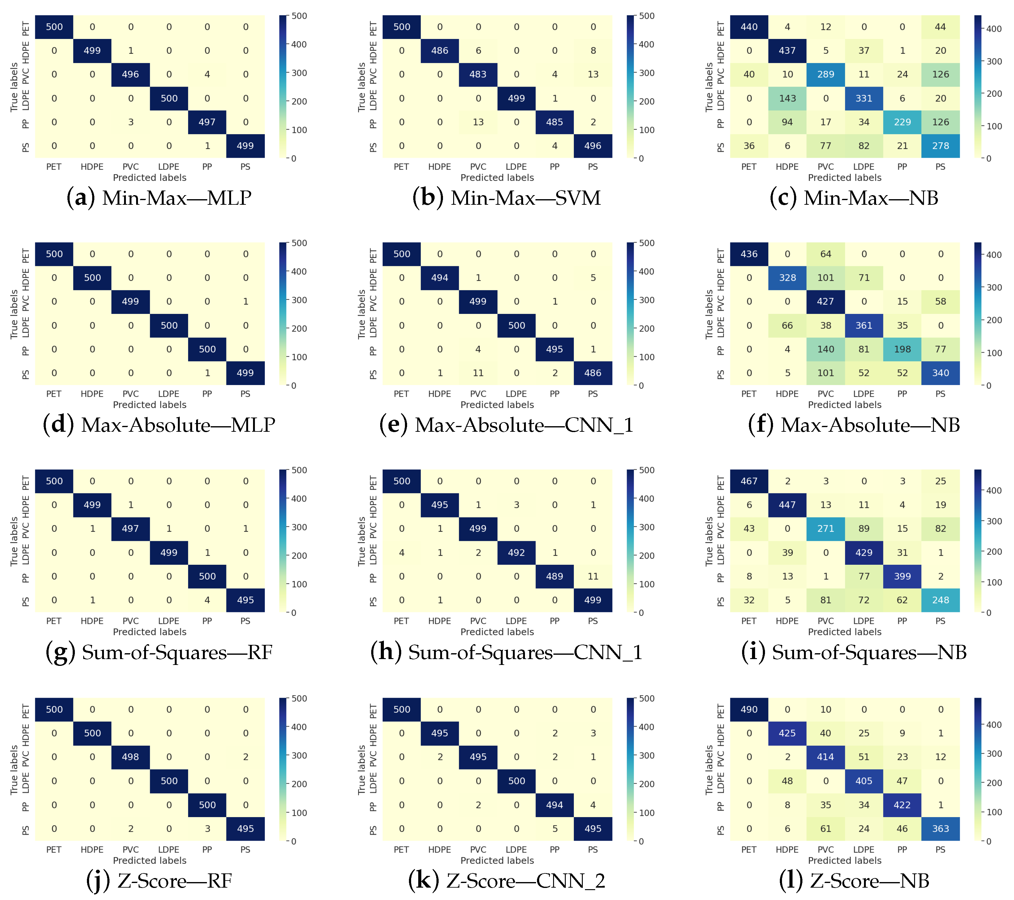
5. Results and Discussion

This section offers a thorough analysis of the effects of various normalization techniques on the performance of machine learning models in microplastic classification using FTIR spectra. Key findings are presented by evaluating metrics such as accuracy, precision, and F1-score, particularly emphasizing the differences in behavior between classical models (including random forest, k-nearest neighbors, and the support vector machine) and advanced neural network models (such as the CNN and MLP). Additionally, the limitations noted in the naive Bayes model are discussed, along with the specific sensitivity of certain algorithms to different normalization schemes. This analysis identifies relevant patterns and establishes the effectiveness of each normalization technique based on the type of model used, providing a strong foundation for selecting optimal preprocessing strategies for spectral data.

5.1. Min-Max Normalization

Min-max normalization yielded outstanding results across most models, with convolutional neural networks (CNNs) and multilayer perceptrons (MLPs) achieving accuracy and precision values between 0.97 and 0.99. Similarly, algorithms such as k-nearest neighbors (kNN), random forest (RF), and the support vector machine (SVM), attained comparable performance levels. In contrast, the naive Bayes model showed significant limitations, with accuracy metrics hovering around 0.69 across all evaluations (

Table 3. Results from machine learning models after applying min-max Normalization. Average and standard deviation values are shown.

Model	Accuracy	Precision	Recall	F1-Score
CNN_1	0.98 ± 0.02	0.99 ± 0.02	0.99 ± 0.01	0.99 ± 0.02
CNN_2	0.97 ± 0.02	0.97 ± 0.02	0.97 ± 0.02	0.97 ± 0.02
MLP	0.99 ± 0.02	0.99 ± 0.01	0.99 ± 0.02	0.99 ± 0.02
kNN	0.98 ± 0.00	0.98 ± 0.00	0.98 ± 0.00	0.98 ± 0.00
Random Forest	0.99 ± 0.01	0.99 ± 0.00	0.99 ± 0.00	0.99 ± 0.00
SVM	0.99 ± 0.00	0.99 ± 0.00	0.99 ± 0.00	0.99 ± 0.00
Naive Bayes	0.69 ± 0.00	0.71 ± 0.02	0.69 ± 0.00	0.69 ± 0.00

).

The superior performance of ML models under min-max normalization indicates that this technique provides a uniform and optimal scale for spectral data, enabling the models to effectively identify complex patterns. However, naive Bayes’ underperformance suggests its inability to manage the non-linear distributions introduced by min-max normalization. This confirms its unsuitability for tasks that require advanced pattern recognition in spectral datasets.

5.2. Max-Absolute Normalization

Max-absolute normalization had a mixed effect on model performance. Algorithms like RF and kNN achieved perfect accuracy and precision scores (1.00), as demonstrated in

Table 4. Results from machine learning models after applying max-absolute normalization. Average and standard deviation values are shown.

Model	Accuracy	Precision	Recall	F1-Score
CNN_1	0.97 ± 0.03	0.98 ± 0.03	0.97 ± 0.03	0.97 ± 0.03
CNN_2	0.81 ± 0.02	0.98 ± 0.02	0.98 ± 0.02	0.80 ± 0.09
MLP	0.96 ± 0.02	0.96 ± 0.02	0.96 ± 0.02	0.96 ± 0.03
kNN	0.99 ± 0.00	0.99 ± 0.00	0.99 ± 0.00	0.99 ± 0.00
Random Forest	1.00 ± 0.00	1.00 ± 0.00	1.00 ± 0.00	1.00 ± 0.00
SVM	0.98 ± 0.00	0.98 ± 0.00	0.98 ± 0.00	0.98 ± 0.00
Naive Bayes	0.62 ± 0.00	0.62 ± 0.02	0.62 ± 0.00	0.61 ± 0.00

. However, deep learning models showed notable variations. CNN_2, in particular, experienced a significant drop in accuracy (0.81) and F1-score (0.80) while maintaining a high precision score. This indicates an increased rate of false positives, possibly suggesting that CNN_2’s architecture is sensitive to the scaling method.

These findings indicate that max-absolute normalization is more suitable for models RF, KNN, and SVM, while deep learning models, particularly CNN_2, may need additional adjustments to adapt to this technique. This sensitivity emphasizes the necessity for hyperparameter optimization or architectural modifications when using this normalization method in deep learning frameworks.

5.3. Sum-of-Squares Normalization

This normalization technique revealed contrasting results among the evaluated models, as shown in

Table 5. Results from machine learning models after applying sum-of-squares normalization. Average and standard deviation values are shown.

Model	Accuracy	Precision	Recall	F1-Score
CNN_1	0.97 ± 0.02	0.97 ± 0.02	0.97 ± 0.02	0.97 ± 0.02
CNN_2	0.71 ± 0.07	0.71 ± 0.09	0.71 ± 0.07	0.69 ± 0.09
MLP	0.85 ± 0.03	0.85 ± 0.02	0.85 ± 0.02	0.85 ± 0.02
kNN	0.99 ± 0.00	0.99 ± 0.00	0.99 ± 0.00	0.99 ± 0.00
Random Forest	1.00 ± 0.00	1.00 ± 0.00	1.00 ± 0.00	1.00 ± 0.00
SVM	0.98 ± 0.00	0.98 ± 0.00	0.98 ± 0.00	0.98 ± 0.00
Naive Bayes	0.62 ± 0.00	0.62 ± 0.02	0.62 ± 0.00	0.61 ± 0.00

. Random forest once again demonstrated optimal performance, achieving perfect scores (1.00) across all metrics. This consistency underscores the robustness of random forest to this normalization method, or possibly even a benefit from it. Conversely, naive Bayes continued to display poor performance, consistent with its results under other normalization methods, further indicating its inadequacy for complex spectral datasets.

CNN_2 experienced a significant decrease in performance with sum-of-squares normalization, as accuracy fell to 0.71. This indicates that the normalization technique may introduce a data scale or distribution that is less favorable for specific architectures, potentially impacting internal computations during training. While MLP models were less sensitive, they showed a slight decline in performance, suggesting a general but less pronounced vulnerability to this normalization method.

5.4. Z-Score Normalization

Z-score normalization emerged as the most robust and effective technique, delivering optimal performance for CNN_1, MLP_1, and RF (

Table 6. Results from machine learning models after applying Z-score normalization. Average and standard deviation values are shown.

Model	Accuracy	Precision	Recall	F1-Score
CNN_1	1.00 ± 0.00	1.00 ± 0.00	1.00 ± 0.00	1.00 ± 0.00
CNN_2	0.99 ± 0.01	0.99 ± 0.01	0.99 ± 0.01	0.99 ± 0.01
MLP	1.00 ± 0.00	1.00 ± 0.00	1.00 ± 0.00	1.00 ± 0.00
kNN	0.98 ± 0.00	0.98 ± 0.00	0.98 ± 0.00	0.98 ± 0.00
Random Forest	1.00 ± 0.00	1.00 ± 0.00	1.00 ± 0.00	1.00 ± 0.00
SVM	0.98 ± 0.00	0.98 ± 0.00	0.98 ± 0.00	0.98 ± 0.00
Naive Bayes	0.62 ± 0.00	0.62 ± 0.02	0.62 ± 0.00	0.62 ± 0.00

). These results indicate that Z-score normalization standardizes the data distribution effectively, enhancing the models’ ability to generalize patterns. However, naive Bayes maintained consistently poor performance, with an accuracy of around 0.62, further reinforcing its limitations for normalized spectral data.

The consistently high performance of CNN_1, MLP_1, and RF under Z-score normalization suggests that this technique provides a strong foundation for machine learning models. Its ability to improve generalization and learning stability underscores its suitability for spectral data analysis.

Figure 2 shows representative examples of confusion matrices that illustrate the performance of classifiers achieving the best, intermediate, and worst results across various normalization techniques. The first column corresponds to the classifier with the top performance in all four normalization scenarios, the second column represents the classifier with intermediate effectiveness, and the third column displays the classifier with the lowest results. The rows indicate the four normalization scenarios.

The purpose of Figure 2 is to provide a detailed and comprehensive overview of the previously reported results. It can be observed that, unlike NB, the other classifiers produce results with minimal error. Additionally, a stable trend is maintained among both the best-performing and intermediate-performing classifiers, with no evidence suggesting that any class is more difficult to learn than another.

On the other hand, NB exhibits the worst performance. We believe this difficulty is not related to the complexity of the spectrum but rather to the nature of the classifier itself, indicating that NB is not the most suitable choice for microplastic classification.

The findings of this research emphasize the relevance of normalization techniques in determining model performance when working with spectral data. Among the methods evaluated, Z-score normalization emerged as the most effective, consistently enhancing the performance of machine learning algorithms. This technique demonstrated a superior ability to handle variability in the data, leading to improved generalization and classification accuracy. In contrast, the naive Bayes model exhibited persistent limitations across all normalization techniques, demonstrating its inability to model the complex relationships inherent in normalized spectral data.

Specific models, particularly CNN_2, showed pronounced sensitivity to specific normalization approaches, revealing the need for further research. Modifications in its architecture or hyperparameters could mitigate these sensitivities, enhancing its adaptability to a broader range of normalization techniques. While min-max normalization proved effective for most models, its simplicity may limit its ability to manage outliers or address complex data distributions as effectively as Z-score normalization.

Random forest (RF) demonstrates strong performance in spectral data classification, achieving accuracy values close to 100% in almost all scenarios. Additionally, its complexity is reduced, as the final trees, on average, utilize only about 40% to 60% of the features. A similar performance is observed in CNN_1 and MLP, which also achieve accuracy values close to 100%. While this could suggest overfitting, we believe these results are primarily due to the high-quality FTIR signals obtained from the studied microplastics, which enabled effective model training.

6. Discussion and Implications

To position our work within the state of the art,

Table 7. Comparison of our work with related research. All references worked at the frame level of the data specter and micro-plastic image.

Ref.	Model	Data Source	Metric	Value	Distinction
[25]	CNN SVM RF k-NN	MIR	Accuracy	100% 100% 98.7% 81.4%	Mid-infrared 12 polymers 4000–1400 cm−1
[26]	LDA PCA	NIR	Precision Recall F1-Score	99–99% 98–93% 98–95%	Near-infrared 4 polymers 50 spectra 1450–1150 nm
[27]	SVM	ATR-FTIR	Kappa Accuracy Precision Recall	99% 71% 87% 99%	ATR 4 Polymers 798 spectra 4000–400 cm−1
[28]	CNN SVM DT k-NN	RAMAN NIR	Accuracy	97% 94% 77.1% 89.9%	2 Espectroscopy techniques 4 Polymers
[21]	CNN	Image	Sensitivity Specificity Precision F-Score Accuracy	56% 91% 63% 60% 61%	400 images sizes 224 × 224
[22]	CNN	Image	Accuracy	82.8	Macroplastics
[23]	CNN	Image	Sensitivity Specificity Precision F-Score Accuracy	56% 91% 63% 60% 61%	Images RGB Sizes 224 × 224 4 polymers
[24]	CNN	Image	Accuracy	74%	Images Sizes 227 × 227
Our work	CNN MLP SVM RF k-NN	FTIR	Accuracy Precision Recall F1-Score	98–100% 98–100% 98–100% 98–100%	6 Polymers 3000 espectra FTIR 4000–400 cm−1

summarizes recent studies that have employed various analytical techniques—including imaging, Raman spectroscopy, MIR, FTIR, and LIBS—alongside machine learning and deep learning models for the identification and quantification of microplastics. While direct comparisons with our experimental results are not feasible due to differences in experimental conditions and dataset characteristics, these studies serve as benchmarks, demonstrating the potential of our approach. Specifically, utilizing broader spectral ranges and increased variability in our samples produces competitive results compared to the state-of-the-art methods for automatic microplastic classification.

As observed in Table 7, FTIR spectroscopy remains one of the most advanced techniques for detecting and analyzing microplastics in environmental samples. Coupled with machine learning and convolutional neural networks (CNNs), FTIR analysis enables the precise identification of microplastics in complex matrices such as water, sediments, and biological tissues. Although many of the methods outlined in Table 7 demonstrate robust performance, our study distinguishes itself by focusing on six common types of industrial plastics, with broader spectral ranges and more significant variability to achieve competitive classification outcomes.

Our reported results, especially those achieved through Z-score normalization, demonstrate the effectiveness of this method in training classifiers for microplastic identification. Importantly, values from the naive Bayes classifier were excluded due to its inadequate performance in classifying microplastics using FTIR spectra.

Future research could examine advanced preprocessing techniques, such as robust scaling or power transformations, to enhance classification accuracy further. Additionally, the relationship between normalization methods and architectural configurations in deep learning models like CNN_2 warrants more in-depth investigation. Hybrid normalization approaches or adaptive scaling mechanisms could increase model robustness and improve the precision of microplastic classification in increasingly complex datasets.

7. Conclusions

This study demonstrated the potential of machine learning tools for classifying microplastics using FTIR-obtained spectra. Six widely used industrial plastics (PET, HDPE, PVC, LDPE, PP, and PS) were analyzed. This work’s primary contribution lies in utilizing broader and more variable spectral ranges than those commonly employed in state-of-the-art research.

Also, a comprehensive comparison of various artificial neural network architectures, including CNN and MLP, was conducted alongside applying classical classifiers such as k-NN, SVM, NB, and RF. The study evaluated different normalization techniques, including min-max, max-abs, sum of squares, and Z-score. Model training and evaluation were performed using the FTIR-PLASTIC-c4 dataset with 10-fold cross-validation to ensure robustness, and an independent dataset was used to validate model performance.

The experimental results highlighted the effectiveness of Z-score normalization, which promoted stable and generalized performance across most models. CNN, MLP, and random forest achieved near-perfect scores in metrics including accuracy, precision, recall, and F1-score. In contrast, the sum-of-squares normalization appeared less effective for artificial neural networks, particularly CNN_2, indicating that this architecture is more sensitive to scale and data distribution.

While traditional algorithms like random forest and k-NN consistently delivered high performance across various normalization techniques, naive Bayes exhibited persistent limitations in all scenarios, reaffirming its inadequacy for analyzing complex spectral data.

Finally, the use of FTIR spectra with broad ranges and high variability enables the accurate classification of microplastics using machine learning techniques. A natural continuation of this work is evaluating these models on significantly smaller microplastics. While this study focused on particles close to 5 mm in size, ongoing research is exploring the classification of plastics with sizes approaching 100 nm. This shift to nanoscale analysis represents a critical step in advancing the detection and characterization of microplastics in increasingly complex and challenging contexts.

References

1. Alimba, C.G.; Faggio, C. Microplastics in the marine environment: Current trends in environmental pollution and mechanisms of toxicological profile. Environ. Toxicol. Pharmacol. 2019, 68, 61–74. [Google Scholar] [CrossRef] [PubMed]
2. Haward, M. Plastic pollution of the world’s seas and oceans as a contemporary challenge in ocean governance. Nat. Commun. 2018, 9, 667. [Google Scholar] [CrossRef] [PubMed]
3. Ai, W.; Liu, S.; Liao, H.; Du, J.; Cai, Y.; Liao, C.; Shi, H.; Lin, Y.; Junaid, M.; Yue, X.; et al. Application of hyperspectral imaging technology in the rapid identification of microplastics in farmland soil. Sci. Total Environ. 2022, 807, 151030. [Google Scholar] [CrossRef]
4. Hopewell, J.; Dvorak, R.; Kosior, E. Plastics recycling: Challenges and opportunities. Philos. Trans. R Soc. Lond. B Biol. Sci. 2009, 364, 2115–2126. [Google Scholar] [CrossRef]
5. Leal Filho, W.; Saari, U.; Fedoruk, M.; Iital, A.; Moora, H.; Klöga, M.; Voronova, V. An overview of the problems posed by plastic products and the role of extended producer responsibility in Europe. J. Clean. Prod. 2019, 214, 550–558. [Google Scholar] [CrossRef]
6. Thompson, R.C.; Moore, C.J.; vom Saal, F.S.; Swan, S.H. Plastics, the environment and human health: Current consensus and future trends. Philos. Trans. R. Soc. 2009, B364, 2153–2166. [Google Scholar] [CrossRef]
7. Rillig, M.C. Microplastic in Terrestrial Ecosystems and the Soil? Environ. Sci. Technol. 2012, 46, 6453. [Google Scholar] [CrossRef]
8. Neto, J.G.B.; Rodrigues, F.L.; Ortega, I.; dos S. Rodrigues, L.; Lacerda, A.L.; Coletto, J.L.; Kessler, F.; Cardoso, L.G.; Madureira, L.; Proietti, M.C. Ingestion of plastic debris by commercially important marine fish in southeast-south Brazil. Environ. Pollut. 2020, 267, 115508. [Google Scholar] [CrossRef]
9. Boerger, C.M.; Lattin, G.L.; Moore, S.L.; Moore, C.J. Plastic ingestion by planktivorous fishes in the North Pacific Central Gyre. Mar. Pollut. Bull. 2010, 60, 2275–2278. [Google Scholar] [CrossRef]
10. Nolan, J.P.; Soar, J.; Zideman, D.A.; Biarent, D.; Bossaert, L.L.; Deakin, C.; Koster, R.W.; Wyllie, J.; Böttiger, B.; Group, E.G.W.; et al. European resuscitation council guidelines for resuscitation 2010 section 1. Executive summary. Resuscitation 2010, 81, 1219–1276. [Google Scholar]
11. Almeshal, I.; Tayeh, B.A.; Alyousef, R.; Alabduljabbar, H.; Mustafa Mohamed, A.; Alaskar, A. Use of recycled plastic as fine aggregate in cementitious composites: A review. Constr. Build. Mater. 2020, 253, 119146. [Google Scholar] [CrossRef]
12. Kuptsov, A.; Zhizhin, G.N. Handbook of Fourier Transform Raman and Infrared Spectra of Polymers; Elsevier: Amsterdam, The Netherlands, 1998. [Google Scholar]
13. Maes, T.; Jessop, R.; Wellner, N.; Haupt, K.; Mayes, A. A rapid-screening approach to detect and quantify microplastics based on fluorescent tagging with Nile Red. Sci. Rep. 2017, 7, 44501. [Google Scholar] [CrossRef] [PubMed]
14. Araujo, C.F.; Nolasco, M.M.; Ribeiro, A.M.; Ribeiro-Claro, P.J. Identification of microplastics using Raman spectroscopy: Latest developments and future prospects. Water Res. 2018, 142, 426–440. [Google Scholar] [CrossRef] [PubMed]
15. Rebelein, A.; Int-Veen, I.; Kammann, U.; Scharsack, J.P. Microplastic fibers—Underestimated threat to aquatic organisms? Sci. Total Environ. 2021, 777, 146045. [Google Scholar] [CrossRef]
16. Nivitha, M.; Prasad, E.; Krishnan, J. Ageing in modified asphalt using FTIR spectroscopy. Int. J. Pavement Eng. 2015, 17, 565–577. [Google Scholar] [CrossRef]
17. Käppler, A.; Fischer, D.; Oberbeckmann, S.; Schernewski, G.; Labrenz, M.; Eichhorn, K.J.; Voit, B. Analysis of environmental microplastics by vibrational microspectroscopy: FTIR, Raman or both? Anal. Bioanal. Chem. 2016, 408, 8377–8391. [Google Scholar] [CrossRef]
18. Munno, K.; De Frond, H.; O’Donnell, B.; Rochman, C.M. Increasing the accessibility for characterizing microplastics: Introducing new application-based and spectral libraries of plastic particles (SLoPP and SLoPP-E). Anal. Chem. 2020, 92, 2443–2451. [Google Scholar] [CrossRef]
19. Ballabio, D.; Consonni, V. Classification tools in chemistry. Part 1: Linear models. PLS-DA. Anal. Methods 2013, 5, 3790–3798. [Google Scholar] [CrossRef]
20. Díez-Pastor, J.F.; Jorge-Villar, S.E.; Arnaiz-González, Á.; García-Osorio, C.I.; Díaz-Acha, Y.; Campeny, M.; Bosch, J.; Melgarejo, J.C. Machine learning algorithms applied to R aman spectra for the identification of variscite originating from the mining complex of G avà. J. Raman Spectrosc. 2020, 51, 1563–1574. [Google Scholar] [CrossRef]
21. Altikat, A.; Gulbe, A.; Altikat, S. Intelligent solid waste classification using deep convolutional neural networks. Int. J. Environ. Sci. Technol. 2022, 19, 1285–1292. [Google Scholar] [CrossRef]
22. Zhang, Q.; Yang, Q.; Zhang, X.; Bao, Q.; Su, J.; Liu, X. Waste image classification based on transfer learning and convolutional neural network. Waste Manag. 2021, 135, 150–157. [Google Scholar] [CrossRef] [PubMed]
23. Bobulski, J.; Kubanek, M. Deep learning for plastic waste classification system. Appl. Comput. Intell. Soft Comput. 2021, 2021, 6626948. [Google Scholar] [CrossRef]
24. Singh, M.K.; Hait, S.; Thakur, A. Hyperspectral imaging-based classification of post-consumer thermoplastics for plastics recycling using artificial neural network. Process Saf. Environ. Prot. 2023, 179, 593–602. [Google Scholar] [CrossRef]
25. Zinchik, S.; Jiang, S.; Friis, S.; Long, F.; Høgstedt, L.; Zavala, V.M.; Bar-Ziv, E. Accurate characterization of mixed plastic waste using machine learning and fast infrared spectroscopy. ACS Sustain. Chem. Eng. 2021, 9, 14143–14151. [Google Scholar] [CrossRef]
26. Jeon, Y.; Seol, W.; Kim, S.; Kim, K.S. Robust near-infrared-based plastic classification with relative spectral similarity pattern. Waste Manag. 2023, 166, 315–324. [Google Scholar] [CrossRef]
27. Yan, X.; Cao, Z.; Murphy, A.; Ye, Y.; Wang, X.; Qiao, Y. FRDA: Fingerprint Region based Data Augmentation using explainable AI for FTIR based microplastics classification. Sci. Total Environ. 2023, 896, 165340. [Google Scholar] [CrossRef]
28. Hufnagl, B.; Steiner, D.; Renner, E.; Löder, M.G.; Laforsch, C.; Lohninger, H. A methodology for the fast identification and monitoring of microplastics in environmental samples using random decision forest classifiers. Anal. Methods 2019, 11, 2277–2285. [Google Scholar] [CrossRef]
29. Coleman, B.R. An introduction to machine learning tools for the analysis of microplastics in complex matrices. Environ. Sci. Processes Impacts 2024, 27, 10–23. [Google Scholar] [CrossRef]
30. Phan, S.; Luscombe, C.K. Recent trends in marine microplastic modeling and machine learning tools: Potential for long-term microplastic monitoring. J. Appl. Phys. 2023, 133, 020701. [Google Scholar] [CrossRef]
31. Zhang, Y.; Zhang, D.; Zhang, Z. A critical review on artificial intelligence—Based microplastics imaging technology: Recent advances, hot-spots and challenges. Int. J. Environ. Res. Public Health 2023, 20, 1150. [Google Scholar] [CrossRef]
32. Kamin, S.N. Programming Languages: An Interpreter-Based Approach; Addison-Wesley Longman Publishing Co., Inc.: Redwood City, CA, USA, 1990. [Google Scholar]
33. Deisenroth, M.P.; Faisal, A.A.; Ong, C.S. Mathematics for Machine Learning; Cambridge University Press: Cambridge, UK, 2020. [Google Scholar]
34. Thomas, R.; McSharry, P. Big Data Revolution: What Farmers, Doctors and Insurance Agents Teach Us About Discovering Big Data Patterns; John Wiley & Sons: West Sussex, UK, 2015. [Google Scholar]
35. Cover, T.; Hart, P. Nearest neighbor pattern classification. IEEE Trans. Inf. Theory 1967, 13, 21–27. [Google Scholar] [CrossRef]
36. Altman, N.S. An introduction to kernel and nearest-neighbor nonparametric regression. Am. Stat. 1992, 46, 175–185. [Google Scholar] [CrossRef]
37. Cortes, C.; Vapnik, V. Support vector machine. Mach. Learn. 1995, 20, 273–297. [Google Scholar] [CrossRef]
38. Shawe-Taylor, J.; Cristianini, N. Support Vector Machines; Cambridge University Press: Cambridge, UK, 2000; Volume 2. [Google Scholar]
39. Pearl, J. Probabilistic Reasoning in Intelligent Systems: Networks of Plausible Inference; Morgan Kaufmann: San Francisco, CA, USA, 1988. [Google Scholar]
40. Friedman, B. Human Values and the Design of Computer Technology; Cambridge University Press: Cambridge, UK, 1997. [Google Scholar]
41. Breiman, L. Random forests. Mach. Learn. 2001, 45, 5–32. [Google Scholar] [CrossRef]
42. Liaw, A. Classification and regression by randomForest. R News 2002, 2, 18–22. [Google Scholar]
43. Goodfellow, I.; Bengio, Y.; Courville, A. Deep Learning; MIT Press: Cambridge, MA, USA, 2016. [Google Scholar]
44. Berzal, F. Redes Neuronales & Deep Learning (Spanish Edition); Apache License: Granada, Spain, 2018. [Google Scholar]
45. Kubat, M. Neural networks: A comprehensive foundation by Simon Haykin. Knowl. Eng. Rev. 1999, 13, 409–412. [Google Scholar] [CrossRef]
46. Block, H.D.; Knight, B., Jr.; Rosenblatt, F. Analysis of a four-layer series-coupled perceptron. II. Rev. Mod. Phys. 1962, 34, 135. [Google Scholar] [CrossRef]
47. Rumelhart, D.E.; Hinton, G.E.; Williams, R.J. Learning internal representations by error propagation, parallel distributed processing, explorations in the microstructure of cognition, ed. de rumelhart and j. mcclelland. Biometrika 1986, 71, 6. [Google Scholar] [CrossRef]
48. Simard, P.; Bottou, L.; Haffner, P.; LeCun, Y. Boxlets: A fast convolution algorithm for signal processing and neural networks. In Advances in Neural Information Processing Systems, Proceedings of the 12th International Conference on Neural Information Processing Systems, Denver, CO, USA, 1–3 December 1998; MIT Press: Cambridge, MA, USA, 1998; Volume 11. [Google Scholar]
49. Krizhevsky, A.; Sutskever, I.; Hinton, G.E. Imagenet classification with deep convolutional neural networks. In Advances in Neural Information Processing Systems, Proceedings of the 26th International Conference on Neural Information Processing Systems, Lake Tahoe, NV, USA, 3–6 December 2012; Curran Associates Inc.: Red Hook, NY, USA, 2012; Volume 25. [Google Scholar] [CrossRef]
50. Walpole, R.E.; Myers, R.H.; Myers, S.L.; Ye, K. Probability & Statistics for Engineers & Scientists; Pearson Education: Boston, MA, USA, 2012. [Google Scholar]
51. Alejo, R.; Antonio, J.A.; Valdovinos, R.M.; Pacheco-Sánchez, J.H. Assessments Metrics for Multi-class Imbalance Learning: A Preliminary Study. In Pattern Recognition, Proceedings of the 5th Mexican Conference, Queretaro, Mexico, 26–29 June 2013; Carrasco-Ochoa, J.A., Martínez-Trinidad, J.F., Rodríguez, J.S., di Baja, G.S., Eds.; Springer: Berlin/Heidelberg, Germany, 2013; pp. 335–343. [Google Scholar] [CrossRef]
52. Fan, M.; Zuo, K.; Wang, J.; Zhu, J. A lightweight multiscale convolutional neural network for garbage sorting. Syst. Soft Comput. 2023, 5, 200059. [Google Scholar] [CrossRef]
53. Villegas-Camacho, O.; Alejo-Eleuterio, R.; Francisco-Valencia, I.; Granda-Gutiérrez, E.; Martínez-Gallegos, S.; Illescas, J. FTIR-Plastics: A Fourier Transform Infrared Spectroscopy dataset for the six most prevalent industrial plastic polymers. Data Brief 2024, 55, 110612. [Google Scholar] [CrossRef]
54. Magaña-Olivé, P.; Martinez-Tavera, E.; Sujitha, S.; Cunill-Flores, J.; Martinez-Gallegos, S.; Sierra, J.; Rovira, J. Evaluation of microplastics and metal accumulation in domestic ducks (Anas platyrhynchos f. domesticus) of a contaminated reservoir in Central Mexico. Mar. Pollut. Bull. 2025, 213, 117639. [Google Scholar] [CrossRef]
Figure 1. Representation of the methodology used for polymer classification from FTIR spectra.
Recycling 10 00046 g001
Figure 2. Representative confusion matrix of the ML performance in the micro-plastic classification.
Recycling 10 00046 g002