Abstract
Batteries are a key resource in the quest for sustainable energy. Here, the theoretical basis is presented for a new type of electrochemical concentration cell that might contribute to this enterprise. The cell, which has been successfully demonstrated in the laboratory, incorporates a chemically asymmetric membrane to drive anisotropic diffusion between two solution chambers; the resulting concentration difference powers the cell. In this study, the membrane’s operation is validated via three theoretical approaches: (i) traditional equilibrium thermodynamics; (ii) balancing drift and diffusion current densities; and (iii) the time-independent diffusion equation. The physical criteria for its operation are developed and its dimensionless variables identified. The cell’s maximum instantaneous power density might exceed W/m. Its self-charging capability should confer multiple advantages over traditional concentration cells (as well as over some voltaics), including improved thermodynamic efficiency, economy, and compactness. Commonalities with other electrochemical systems (e.g., liquid chromatography, metal corrosion, and solid state diodes) are discussed, and a physical instantiation of the cell is reviewed. Recent numerical simulations corroborate its essential processes.
1. Introduction
Electrochemical cells are hallmarks of modern civilization and are also among its oldest technologies, dating back at least to 1790, in the research of Galvani and Volta [1,2,3,4]. They serve in all technological strata and have become crucial to the rise of sustainable energy; their worldwide power storage capacity is currently 1–2 GW—and is rising exponentially [4]. It is estimated that spending on galvanic (voltaic) storage systems exceeds 100 billion USD per year, while additional billions are devoted to their research and development, making them among the most intensely studied physical systems in the world.
Electrochemical cells come in several varieties. The most common, voltaic cells, transduce chemical energy into electrical energy; in fact, almost any chemical reaction involving the transfer of electrons can be parlayed into a battery. Voltaics transfers electrons between disparate chemical species such as, for example, in the hydrogen–oxygen fuel cell: 2H + O⟶ 2HO. In contrast, a concentration cell generates electricity from the concentration difference between two samples of a single chemical species, exploiting their entropy of mixing.
Concentration cells usually provide smaller emfs than voltaics (e.g., ∼ V vs. ∼1 V) and lower energy densities as well (e.g., ∼– J/m vs. ∼ J/m). Nevertheless, large-scale concentration cells have found niche applications [5,6,7]. To illustrate this, the chemical potential attainable when playing the salinity of seawater against that of fresh water (e.g., where a river flows into the sea) is comparable to the gravitational potential of a 200 m-high dam. However, because traditional free energy sources are richer, exhibit larger emfs and energy densities, and are usually easier and less expensive to tap, concentration cells are often overlooked. This is an undeserved oversight.
In nature, concentration cells and gradients are ubiquitous and crucial sources of energy. For instance, salinity gradients are partially responsible for thermohaline circulation in the world’s oceans, which is integral to global heat and matter transport, as well as to climate stability [8]. Proton gradients across biological membranes store electrostatic potential energy and are converted into chemical energy, the most famous example of which is oxidative phosphorylation in mitochondrial membranes of eukaryotes, in which ADP is converted into ATP [9]. Action potentials (nerve impulses) stem from the relaxation of sodium and potassium ion gradients across membranes of various so-called excitable cells (e.g., neurons, muscle cells, endocrine cells) [10]. Nature loves concentration gradients and life is predicated on them.
This study develops the theory of a new type of concentration cell [11]. This asymmetric membrane concentration cell (AMCC) generates electricity identically to traditional concentration cells, but it is distinguished by the nonstandard means by which its concentration difference is established and maintained (). Here, is expressed in mole/liter (i.e., molarity) or in particles/m. In traditional cells, is arranged externally via prepared solutions, thereby incurring costs in thermodynamic work, while in an AMCC it is generated internally, tapping thermal energy within the cell itself to promote anisotropic molecular diffusion of ions (or neutrals) through a chemically asymmetric membrane. This process entails no external thermodynamic work and it confers several potential advantages over its competitors, including improved economy, thermodynamic efficiency, and compactness. The AMCC concept can be applied to many types of concentration cells [5,6,7] and perhaps even to some types of voltaics [1,2,3]. This has been successfully demonstrated in the laboratory [11], and numerical simulations strongly corroborate its basic physical processes [12]. Either neutral or ionic species can be active solutes; here, for explanatory simplicity, we consider neutral species only.
The heart of the AMCC is a chemically asymmetric membrane that establishes an equilibrium concentration gradient. The physical and chemical assumptions that lead to it are unremarkable, but the resulting effect—self-chargeability—is surprising and novel.
In this study, the membrane’s operation is validated by three complementary theoretical approaches: (i) traditional equilibrium thermodynamics (Section 2.1); (ii) competition between drift and diffusion current densities (Section 2.4); and (iii) solutions to the time-independent diffusion equation (Appendix A). The physical criteria and dimensionless parameters governing its operation are derived (Section 2.2 and Section 2.3). Dimensional analysis suggests that its maximum power density could be substantial, perhaps in excess of W/m. Similarities to other electrochemical and physical systems (i.e., liquid chromatography, metal corrosion, and solid state diodes) provide additional insight into its character.
This article is organized as follows: Section 2 develops the thermodynamics of the AMCC concentration gradient; Section 3 discusses analogies to semiconductor systems as well as connections to metal corrosion and chromatography; and Section 4 summarizes the main results and proposes directions for future research. Appendix A outlines an approach to deriving the concentration gradient using the time-independent diffusion equation, and Appendix B reviews a physical instantiation of the AMCC.
2. Theory
The AMCC generates electricity from a concentration difference produced by a chemically asymmetric membrane. It consists of two subsystems: (i) the asymmetric membrane separator (AMS), which generates the concentration difference between two liquid reservoirs; and (ii) the concentration cell that converts this into electricity. The former is the focus of this study; the latter is extensively described elsewhere [1,2,3,4,5,6,7] and so will be considered only incidentally.
The AMS can be analyzed from several viewpoints. In this section, it is developed from a thermodynamic perspective as an array of chemically reactive microscopic tubes that generates an equilibrium gradient in solute concentration.
2.1. AMS Model: Tube Array
The AMS consists of two thin liquid reservoirs separated by a chemically asymmetric membrane. Here, the membrane is modeled as an array of hollow, large aspect ratio tubes bundled together lengthwise like a sheaf of wheat and filled with species A dissolved in a solvent, e.g., water, methanol or acetone (Figure 1a). Typical tube dimensions are in the range: m m and m m. Billions or trillions of tubes can comprise a single AMS membrane. They are assumed to be straight and uniform, thereby sidestepping issues of tube tortuosity and constriction, both of which complicate, but do not illuminate, the essential physics. The liquid reservoirs are sufficiently thin that their A concentrations are dominated by those that suffuse the membrane. The tubes are identical; therefore, to understand the physical chemistry of a single tube is to understand that of the entire membrane.
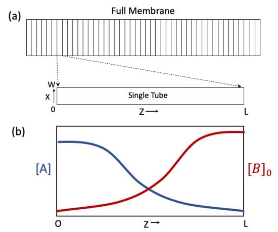
Figure 1.
Depictions of AMS membrane and species concentration profiles. (a) Cross section of full membrane modeled as an array of microscopic tubes (top) and magnification of a single tube extracted from the membrane and rotated for clarity (bottom). (b) Plot of initial distribution of binding sites ( in red) and resultant equilibrium concentration of solute ( in blue) along the length of the tube (). Here, the distributions are portrayed as sigmoid functions. Reciprocal spatial relation between and follow from equilibrium considerations, Equations (2)–(5). The concentration differential (), powers the AMCC.
Firmly secured to the inner walls of each tube are chemical binding sites B that undergo the following reversible chemical reaction with the solute molecule A:
Species A is dissolved in a liquid solvent (l), while species and B are bound surface states (s) on the tube’s wall. The initial number of chemically active species embedded on the tube’s inner surface () is comparable to the total number of A molecules () in the tube. This total initial number of A molecules can be expressed as , with being a differential volume in the AMS tube; represents the initial uniform concentration of A in the tube before binding begins. The total number of initial binding sites is, likewise, , with being a differential area on the AMS tube’s inner wall.
For this discussion, it is assumed that species A, B and the solvent molecules interact via standard intermolecular forces (e.g., polar electrostatic, hydrogen bonding, van der Waals).
A unique equilibrium will arise inside the AMS membrane and, by extension, in the two reservoirs. The equilibrium constant for the reaction in Equation (1) is [13,14]:
where is the Gibbs energy change for the reaction (J); J/K is Boltzmann’s constant; T is the absolute temperature (K); thus, is the thermal energy and . Here, is the volume concentration of species A (molecules/m), while and are surface concentrations of species B and complex (molecules/m). These concentrations are normalized appropriately (e.g., against one molar concentrations), thus rendering dimensionless.
The initial distribution of open binding sites before reacting is and, after binding to some A molecules, it is reduced to . (Note: At equilibrium, ). A useful expression for can be derived from Equation (2) by noting that and are linked: for every AB complex formed, one B site is lost; that is, . One has, therefore, With this in mind, Equation (2) can be recast as:
In principle, the following quantities in Equation (3) can vary axially (along coordinate z), thereby rendering a function of z: (i) the initial surface number density of B, ; (ii) the surface number density of B evolving toward equilibrium ; and (iii) the local liquid-surface equilibrium constant, (or equivalently the free energy of binding, ). Assuming all vary axially, the variation in along the length of the tube can be written:
or equivalently in terms of Gibbs energy:
Here, is the equilibrium concentration gradient of A along the length of the tube, hence the concentration gradient for the AMS. When properly engaged, it powers the AMCC. Usually, equilibrium is the state in which concentration gradients are absent, but this is not the case for the AMS; rather, here a concentration gradient is the condition of thermodynamic equilibrium. Other examples of equilibrium concentration gradients are examined in Section 2.4, Section 3.1 and Section 3.2.
Equations (4) and (5) indicate that () can be induced either by varying the areal number density of binding sites () or by varying the equilibrium constant () (or equivalently, the Gibbs energy, ). The former can be accomplished by locally seeding the walls with B appropriately at the start, while the latter can be achieved by grading the physical–chemical characteristics of species B itself. For example, if A is the hydrogen ion H and B is a carboxylate ion (COO), then the binding strength of H to COO can be adjusted by several means. For instance, if COO is attached to a carbon skeleton, functional groups can be attached at specific locations along the carbon framework to alter its acidity. As an illustration, consider the increase in pKa for the first three carboxylic acids: formic (one carbon; pKa = 3.75); acetic (two carbons; pKa = 4.74); propionic (three carbons; pKa = 4.87). This corresponds to a variation in by a factor of 13 between formic and propionic acids. By adding other functional groups nearby (e.g., alcohol, ketone, amine), the carboxylate’s pKa can be further tailored along the length of the tube.
A hallmark of thermodynamic equilibrium is balance between competing processes, reactions, and forces. The equilibrium concentration gradient is no different. If the for the surface reaction (Equation (1)) increases monotonically along the tube from left to right (Figure 1b), then the first term on the rhs of Equation (4) is negative definite, signaling larger on the left than on the right (Figure 1b). Likewise, if increases monotonically from left to right, then the second term on the rhs of Equation (4) is positive. (This can also be inferred from Le Chatelier’s principle applied to the reaction). Together, these countervailing tendencies limit the concentration gradient.
Once a concentration gradient has been established by the AMS, electrodes and an electrical load can be engaged to form a concentration cell, thus completing the AMCC. (See the example in Appendix B). The emf for a concentration cell ((V)) is given by the Nernst equation:
Here, is the emf (V); p is the transfer number (the number of electrons transferred in the reaction, here taken as ); q is an electronic charge ( C); is the high (low) concentration of A, and is the chemical activity coefficient for the high (low) concentration (unitless). For dilute species, . At T = 300 K, increases roughly 59 mV per decade difference between , and the thermal voltage is mV.
A few items of note:
- (1)
- The concentration pertains to volume, while , , , and pertain to the surrounding surfaces. As such, this is a boundary value problem, in which the specifics of and can depend heavily on the size and shape of the reaction vessel (membrane channels). Numerical simulations bear this out [12].
- (2)
- Analysis leading to Equations (3)–(5) does not explicitly include the effects of Brownian and Fick’s diffusion of species A along the tube, both of which should attenuate . This attenuation has been observed in numerical simulations [12] and is corroborated by experiments [11].
- (3)
- While Equations (4) and (5) indicate that the magnitude of is proportional to , numerically large gradients do not necessarily translate to larger emfs because the Nernst relation (Equation (6)) dictates that it is the ratio that determines emf, not their individual magnitudes. (For instance, contrast the following two scenarios: (i) M and M versus (ii) M and M. The concentrations of the latter are 50–400 times greater than the former, but the Nernst emf of the former is greater than the latter by a factor of 2).
2.2. Maximizing AMS Density Gradients
The density gradient is the sine qua non of the AMS and AMCC. Strategies for maximizing it can be inferred by considering various operating limits of the AMS indicated by Equations (2)–(5).
- Limit 1: Trivially, if the AMS tube has an initially uniform axial concentration of B (i.e., ) and also uniform binding strength (i.e., ), then the concentration of A in solution will also be uniform (i.e., ), thus the AMS fails.Conclusion: At least one of the parameters, or must vary axially.
- Limit 2: If the binding is too strong, such that effectively, , then, assuming remains finite, the first term on the rhs of Equation (4) goes to zero, while the second term becomes irrelevant because A–B binding is effectively permanent, in which case there is no ongoing interplay between the walls and solute. Thus, A diffuses to uniform concentration (), and again, the AMS fails.Conclusion: Very strong surface binding should be avoided.
- Limit 3: In the opposite limit (very weak, effectively no surface binding), the walls are operationally inert, and therefore lack any chemical asymmetry, so and along the tube. As a result, A molecules diffuse freely, uniformly filling the tube, rendering .Conclusion: Weak binding should likewise be avoided.
- Limit 4: If , then regardless of the reactivity of A for B, the concentration of B will not change appreciably (), in which case Equation (3) gives . In this scenario, species A has been stripped from the solution, precipitated out as ; thus, the AMS fails.Conclusion: should be avoided.
- Limit 5: In the opposite limit, if , then the initial concentration of A is effectively unchanged (i.e., ). Without sculpting by [B(z)], the concentration of A will become uniform along the length of the tube via diffusion, in which case , and again the AMS fails.Conclusion: should be avoided.
Clearly, the success of the AMS calls for moderation, as implied by the limiting conditions not conducive to it. Specifically, the limits to be avoided are:
- (i)
- (ii)
- (iii)
- (iv)
- (v)
- (vi)
These criteria follow naturally from Le Chatelier’s principle and also comport with Sabatier’s principle for catalysts [15,16].
Further criteria for the AMS can be inferred, involving temporal and spatial conditions. A necessary condition for non-zero and is that species A come into local chemical equilibrium with the tube walls either: (a) on an equilibration time scale short compared to A’s diffusion time down an appreciable length of the AMS tube ( for Brownian diffusion, with being the diffusion coefficient for A in solution (m/s)); or equivalently, (b) on a distance scale short compared to an appreciable length of the tube (L). (The truth of this criterion can be seen by considering its opposite: If A diffuses along the tube so rapidly that it cannot come to chemical equilibrium with the walls locally, then the solute-wall reaction becomes an average value along the tube length. With the chemical reactivity effectively symmetrized axially, one has , thus vitiating the AMS, as per Limit 1). The chemical equilibration time () is the time required for A molecules to diffuse to the walls and to come into equilibrium with them and their binding sites B. The diffusion time is the time necessary for A in the bulk solution to diffuse the diameter of the tube (). Although just a few wall collisions may suffice to complete an reaction, chemical equilibrium cannot be consummated until a steady state is reached between adsorption and desorption, which suggests that must be at least as long as A’s residence time on the binding site B, . (For gas-surface reactions, the residence times for physisorbed or weakly chemisorbed organics (10–20 kcal/mole) are typically s s, which overlap well with characteristic diffusion times for proposed AMS membranes. Liquid-surface residence times should be comparable). Furthermore, species A should reside on the surface long enough for diffusion along the tube to differentiate between regions of differing residence times; separation by perhaps a few w might suffice. In this case, a condition for non-zero or becomes (). The original condition (a) meanwhile, requires (). Putting these together, one has and , the latter indicating that tubes should have large aspect ratios.
The limiting conditions (iii)–(vi) suggest that neither A nor B should chemically dominate the other and that, to some degree, they should be comparable in number ()—perhaps not equal, but probably within a few orders of magnitude of each other [17,18,19]. Furthermore, if large is sought, a large initial is indicated and this, in turn, points to relatively large surface-to-volume ratios for the tubes such that . For this criterion, bundles of long, microscopic- or nanoscopic-diameter tubes are optimal.
2.3. Dimensionless Constants and the Buckingham Pi Theorem
The behavior of the AMS tube is governed largely by the following six independent variables:
- (1)
- : total number of A molecules in the AMS tube. (Dimensions: None).
- (2)
- : initial density distribution of binding sites B as a function of axial location (z) along the tube walls. (Dimensions: m).
- (3)
- : residence time of A on binding site B as a function of axial location (z) along the tube. Here, appears as a proxy for or . (Dimensions: s).
- (4)
- w: diameter of AMS tube. (Dimensions: m).
- (5)
- L: axial length of AMS tube. (Dimension: m).
- (6)
- : Diffusion coefficient for species A in solution. (Dimensions: m/s) Typical value: m/s for small molecules and ions in water.
The AMS possesses three characteristic time scales (, , and ), two characteristic length scales (w and L), and three characteristic particle numbers (, , and ), only two of which are independent (i.e., ). Two of the characteristic time scales are linked to the length scales: i.e., and .
The number of dimensionless variables that define this system is set by the Buckingham Pi theorem (BPt) [20]. Because there are six independent variables (, , , w, L, and D) expressed in terms of two dimensional units (m, s), the BPt predicts four dimensionless variables. The tube aspect ratio, has already been identified: , based on considerations of diffusion times. Residence time () is the only independent variable solely involving time, so another time-dependent term must be invoked to create a dimensionless variable; here, is the natural choice, given the central role of diffusion. As discussed earlier, cannot be inordinately long, but must be long enough to have thermodynamic effect. Additionally, the progression of characteristic times should be roughly: . This suggests two dimensionless variables satisfying inequalities: and .
Finally, as discussed above, species A and B should compete with, but not dominate, each another; thus, they should be somewhat comparable. This suggests a third dimensionless variable :
where the integrations are over the interior area and volume of the AMS tube. With these, the AMS’s operational regime can be circumscribed with the following four dimensionless parameters:
- (1)
- ;
- (2)
- ;
- (3)
- ; and
- (4)
- .
In addition to framing the operational limits of the AMS, these inform the numerical model of the membrane [12].
2.4. Equilibrium Current Densities in the AMS
The asymmetric membrane concentration cell (AMCC)—or any concentration cell, for that matter—requires two reservoirs at distinct concentrations in contact with its anodic and cathodic electrodes. Creating a spatial gradient in the solute concentration is the fundamental requirement; it is the arete of the AMS. As shown in Section 2.1, traditional thermodynamics demonstrates this gradient can arise naturally as the equilibrium state in an AMS tube.
Here, it is shown that this equilibrium state can also be viewed as the balance between oppositely directed one-dimensional current densities of species A within the AMS tube, one due to particle diffusion, the other due to the gradient in the chemical potential imposed by the asymmetric wall composition. (The condition of current balance is regularly used to derive equilibrium states involving diffusion).
Diffusion current density, written based on Fick’s law, is: , where is the diffusion constant for A. The drift current density, driven by a chemical potential gradient, can be written: , where is the axially varying Gibbs free energy per reaction (J), and is the mobility of A. (For neutral A, the units of mobility are (s/kg).)
The diffusion and currents are oppositely directed, and at equilibrium, they balance each other. Setting them equal () and appealing to the Einstein relation (), one obtains:
Here, and . Following the left-right convention in Figure 1, and because for the binding reaction (A + B⇌), one has , indicating an equilibrium concentration difference between the ends of the tube, the defining feature of the AMS (Figure 1b). (If one unpacks differently, one can obtain Equations (2) and (3)).
This result is not surprising. Equation (8) is a chemical analog of an exemplar: the vertical distribution of molecules in an isothermal atmosphere in a uniform gravitational field, which is written as follows: . Here, m is the mass of an individual A gas molecule (kg); g is the gravitational acceleration (m/s); z is the vertical altitude (m); and is A’s concentration at sea level. Clearly, the gravitational potential energy of A varies with altitude (). In an AMS the chemical force on A (i.e., ) can be billions of times stronger than the gravitational force (i.e., ); hence, can change appreciably over sub-micron distances as opposed to over hundreds or thousands of meters in a planetary atmosphere. Additionally, the functional dependence of is more flexible than that of the gravitational potential. For instance, if G is constant, then . There is no gradient, therefore no chemical force, in which case diffusion erases all concentration gradients in the solution; thus, the AMS and AMCC fail. (In the gravitational case, this corresponds to no gravitational field, in which case the gas number density will be uniform). If the Gibbs energy varies linearly with z (i.e., , with a constant (kg·m/s), then varies exponentially like an isothermal atmosphere (, with an e-folding distance .
For a robust AMCC, should be sufficiently short that multiple e-foldings accrue along the length of the AMS tube so as to attain a large concentration difference in A, while still maintaining reasonably short diffusion times. (Recall that diffusion times typically scale as the variance of the displacement: , where n is the system’s dimensionality, n = 1, 2, or 3). To illustrate, an increase in concentration by a factor of 100 along the tube requires that the binding energy of species A must decrease by roughly over that distance. This can be arranged via or , as discussed earlier (Section 2.1). Overall, in contrast with gravitational potential, can exhibit a good deal of functional flexibility consistent with an effective AMS.
In summary, this section provided two complementary derivations of the concentration gradient induced by the AMS: the first from equilibrium thermodynamics, the second via current balance. The system’s dimensionless constants and optimum operating regimes were also identified.
3. Discussion
The AMS is closely related to several well-known chemical, electrochemical, and solid state systems. In this section these are examined.
Starting at the molecular level, the AMS membrane can be likened to an extended, macroscopic version of a diprotic acid that has functional groups with disparate acidities. Just as a diprotic acid can display different acidities at opposite ends of the same molecule (e.g., linear perfluoropentadecane with a carboxylic acid group at one end and a sulfonic acid group at the other), likewise, an AMS membrane, by virtue of its construction and composition, can also be made more acidic on one side than on the other; that is, it can present disparate chemical activities on opposite sides of the same structure [21] and, thus, create a concentration gradient [11].
3.1. Liquid Chromatography and Concentration Gradient Corrosion
The chemical principles undergirding the AMS have well-established precedents. Liquid chromatography [22,23], for example, is based on the disparate sticking strengths and retention times of different solute molecules on a column’s substrate chemicals; this is what separates them spatio-temporally and allows them to be collected and identified. The AMS membrane operates similarly—binding differentially to a solute molecule across its thickness—but with the outcome of creating an equilibrium concentration differential (gradient) there. In many respects, one can think of the AMS as a static version of a chromatographic column.
The wide variety of liquid-based chromatographies [22,23] attest to the variability and controllability of surface binding site densities, binding energies, and residence times. The AMS tube operates similarly to a standard chromatographic column, with the following caveats: (a) binding sites B are inside the membrane rather than on the surfaces of beads in a column; (b) and are graded axially rather than being constant; (c) the desired product () is a static, equilibrium fluid, rather a nonequilibrium fluid flow; and (d) the AMS equilibrium is achieved via passive diffusion.
The AMCC can also be understood in terms of one of the most ubiquitous and costly types of corrosion: concentration gradient corrosion (CGC) [24,25,26], which commonly arises in aqueous environments with faying metal surfaces. (The worldwide annual cost of corrosion of all types is estimated to be more than a trillion dollars USD; in the US alone it has been estimated to account for more than 3% of GDP). For example, beneath an angle joint bolted to a metal base, dissolved metal ions are often concentrated compared with adjacent areas. This metal ion concentration gradient over a single piece of metal constitutes a concentration cell, one that corrodes the metal in contact with the high ion concentration and deposits metal in the low-concentration region. (CGC can also arise from gradients in dissolved atmospheric oxygen rather than from metal ions.) In our metal-centric civilization, we are surrounded by electrochemical corrosion, most of it unwanted, unregulated, and unprofitable—and a fair bit of it CGC.
The AMCC is a controlled and useful version of CGC. The AMS purposefully establishes a concentration gradient, while the AMCC electrodes undergo electrochemical reactions that relax the gradient; specifically, the anode protects and the cathode corrodes. Their differences, however, are noteworthy. First, whereas the CGC is uncontrolled, the AMS has well-defined current–voltage characteristics and mass transfer; it can be engineered and tuned. Second, and more importantly, whereas CGC is undesirable, ecologically destructive and economically costly, the AMCC is ecologically benign and potentially valuable as an energy source.
The AMCC should demonstrate several advantages over other types of concentration cells—and perhaps even over some voltaics. First, the AMCC’s is self-generated and internal, rather than imposed by external means that require work input and chemical replenishment. This should simplify its operation, reduce support apparatus, and improve its overall efficiency. Second, if the AMS solutions are removed to power a concentration cell and then returned to the AMS, their s should return to their original values because this is the equilibrium state of the system. This recurrence is spontaneous, mediated by thermal diffusion through the AMS membrane. In effect, with respect to its working solutions, the AMCC is self-charging.
The rechargeability of the AMS solution has been verified experimentally by this author (Figure 3, Ref. [11]) as well as by an independent laboratory. Original experimental membranes rechargeably generated only 1–2% concentration differences, while more recent experiments utilizing commercial bipolar membranes (Fumasep BPM in M NaCl solutions) have demonstrated rechargeable concentration differentials up to nearly 50% differences.
Note that although the AMS solution is rechargeable, the full AMCC is not. As noted earlier, the AMCC is a case of controlled corrosion (CGC). As in the rudimentary example of Appendix B, its electrodes do not reconstitute themselves; rather, the anode continually precipitates Cl as AgCl, accruing mass, while the cathode continually loses mass. As a result, the AMCC’s operation does not constitute a closed thermodynamic cycle and does not undercut the second law of thermodynamics. (The Kelvin-Planck form of the second law can be stated: A quantity of heat cannot be converted solely into work in a thermodynamic cycle).
The net mass transfer between electrodes ultimately exhausts the free energy of the AMCC, unless its electrodes are occasionally swapped. However, even without this maneuver, the AMCC might offer increased service life and economy over traditional concentration cells. If it is fitted with an oversized cathode, then unlike conventional cells, which must be refilled after discharge, the AMCC should run multiple discharge–recharge cycles without refueling solutions, until the cathode is consumed. Its economy and compactness would thereby be improved because it requires less support apparatus for recharging, e.g., external circuits, plumbing, storage tanks.
A fundamental aspect of the AMS and its self-charging capability is that concentration cells operate at very low—at literally thermal—emfs. (Recall that at T = 300 K, mV). Along the entire length of an AMS, might reach only 4–5 kT of energy. Additionally, thermal energy drives diffusion in fluids and membranes, and it is also sufficient to support solvation reactions such as acid association–dissociation. Because it is ultimately powered by ambient thermal energy, the AMCC might be called a thermal battery as well as a concentration cell.
3.2. Analogy to Solid State Diodes
In several respects, AMS operation is analogous to that of solid state p–p diodes. The correspondences between bipolar membranes (BPMs) [27,28,29,30,31,32,33], ion exchange membranes and traditional solid state n- and p-doped semiconductors, diodes and transistors have been noted by others [34]. In fact, membranes and solutions have been fabricated into ionic diodes and ionic transistors and even ionic circuits [35,36,37,38,39,40]. The AMS and AMCC are natural extensions of these. The novel characteristic here is that the AMS generates a concentration gradient that performs as a free energy source for the AMCC. A full account of the correspondences between the two fields is beyond the scope of this paper; however, a few instructive introductory remarks are instuctive.
The built-in potential across a standard heterogeneous p–n semiconductor diode () is given approximately by the semiconductor version of the Nernst relation [41,42]:
where (m) are the heterogeneous acceptor/donor concentrations and is the intrinsic carrier concentration of the semiconductor (in silicon at 300 K, m). For a representative case ( m and m in silicon), one has V.
Though often not appreciated, semiconductor diodes can also be fabricated homogeneously; that is, made completely from p-pure or n-pure materials – analogously to how an AMS employs a single chemical species. In this case, the built-in potential is given by:
where (m) are the high/low concentrations of the single species. (Note the similarity to Equation (6)). A purely p-doped silicon diode with identical concentrations to the above silicon p-n diode gives V for the p–p diode. Notice, too, the similar reduction in potential when switching from heterogeneous to homogeneous diodes (0.8 V vs. 0.2 V), which mirrors the difference in between typical voltaic and concentration cells.
This analogy runs deeper. The depletion region of the p–p diode is an electrophysical analog of an AMS membrane. Whereas the diode’s depletion region and its are the results of a difference in chemical potential and concentration between the p and p regions (carrier reservoirs) relaxing to chemical equilibrium, in the AMS, the chemical potential difference is built into the membrane itself, which then relaxes to equilibrium by generating concentration imbalances between the two thin solution reservoirs at their ends. The Nernst equation describes both systems. (The Nernst equation and its variants are central to almost all chemical, plasma, and semiconductor systems). Effectively, the AMS and p–p diode are inside-out versions (inversions) of one another. In the p–p diode, the species concentration differences in the bulk (i.e., ) determine the character of the interface (depletion region), whereas in the AMS, it is the inverse: the character of the interface (membrane) determines the species concentration differences in the bulk ().
The spontaneous recharging of the AMS is also analogous to the spontaneous recharging in semiconductor systems involving pn junctions. Both are driven by gradients in chemical potentials and are mediated by diffusion. It is well known that an equilibrium-state electric field resides at the junction between p-doped and n-doped regions of static semiconductors (the so-called depletion region) and is due to the thermal cross-diffusion of p- and n-type charge carriers. These fields can be modified by perturbing the diode’s electronic or mechanical boundary conditions [43,44]. However, when these perturbations are removed, the electric fields spontaneously revert to their original values because, after all, they represent the equilibrium state for the original configuration. (This reversion is typically rapid, often taking just 10–100 ns). Likewise, when the s are expended in the AMCC’s concentration cell, they are re-established when returned to the AMS. The implications of this are intriguing, particularly as they pertain to the second law [43,44].
To be clear, the membrane processes that generate concentration differences are independent of the chemical reactions at the electrodes; furthermore, by themselves they cannot drive electric currents. In fact, the membrane and the electrodes serve cross-purposes: the membrane generates concentration gradients, while the electrodes destroy them.
The depletion regions of pn or pp diodes harbor electrostatic potentials and strong electric fields; however, it is well known that these cannot be parlayed directly into electric current because they are artifacts of the diode reaching thermal and chemical equilibrium—a state at which there is no capacity for particle transport. On the other hand, proposals exist for converting this diodic electric field energy into mechanical motion which can then be transduced secondarily into electricity, for example, via the Faraday effect [43,44]. Such proposals are theoretical and have not be verified experimentally. Analogously, the AMS naturally creates a concentration gradient that is also an equilibrium state of the system and which, by itself, cannot directly produce electric current. However, with the employ of suitable electrodes and surface reactions, electricity can be generated from the membrane-induced gradient. This scenario has been verified experimentally [11].
3.3. AMCC Energy and Power Density
Energy and power densities are standard metrics for battery performance. Energy density (J/m) indicates how much work can be achieved by a battery of a given volume, whereas power density (W/m) indicates how fast that amount of work can be completed. In terms of , the AMCC, like other types of concentration cell, should be inferior to standard voltaics by roughly 2–3 orders of magnitude; however, its power densities might be comparable to that of commercial voltaics (e.g., (lithium-ion) W/m). An estimate of AMCC power density () can be made as follows. Assume , where is the cell emf given by the Nernst relation, Equation (6); I is the particle diffusion current in an AMS tube (; is the cross-sectional area of the tube; and is the tube volume (Figure 1). Here, is the particle diffusion current density (particles/m s), as per Fick’s law [45]. (It is assumed that the AMCC power output is diffusion-limited, expressed through . Furthermore, it is assumed that the density gradient scales roughly as: ).
Invoking the Einstein relation (), where (C·s/kg) is the charge mobility, the AMCC power density (W/m can be shown to scale as:
The last form is revealing: thermal energy () and size (L) appear quadratically. Both the Nernst emf and the diffusion current contribute a term; clearly, this system is thermally driven. Small device length L, high species mobility , elevated temperatures, and high concentration () also favor large . Of these, L is probably the parameter most amenable to engineering improvements: thin membranes and reservoirs are advised.
As a concrete example of , assume the hydrochloric acid AMCC above [11], with pH = 1, a pH = 1 (concentration factor of 10), the diffusion coefficient of aqueous chloride ions ( m/s), and cell size (m). With these, Equation (11) predicts a maximum power density in excess of W/m. Standard inefficiencies in fluid and heat transfer, however, as well as electrochemical nonidealities, should reduce this number significantly. Engineering issues surrounding this will be considered in future investigations.
Quantitative comparisons can be made between this theory and recent experiments [46]. Small, single-cell AMCCs using commercial bipolar membranes sodium chloride solutions (volume = m; Fumasep BPM membrane; M NaCl) have generated voltages in excess of V and currents greater than A, indicating power densities of roughly W/m, values significantly below the theoretical limits derived above. Solute concentration ratios inferred from the Nernst equation (Equation (6)) are likewise modest: . It should be borne in mind that these cells are experimental and have not been optimized for power with respect to membrane thickness, composition or porosity, nor with respect to solute concentration or type.
Energy densities (J/m) for a single-discharge AMCC should be inferior to those of standard voltaics by 2–3 orders of magnitude ((Lithium-ion) J/m). However, because the AMCC is self-charging, its integrated energy density (energy summed over all discharge–recharge cycles) should be superior to other types of concentration cells and, if it can complete – thermo-chemical cycles before its electrodes are exhausted, it might be comparable to commercial voltaics.
It will be interesting to see whether the AMS self-charging concept can be transplanted to voltaic cells with their larger emfs and energy densities. While this cannot yet be ruled out, there are good theoretical reasons to doubt its success. The thermal energy density of a material (excluding phase transitions) scales as , where is the particle number density (m). For T = 300 K, the thermal energy of a molecule is roughly a few J eV. (Here, vibrational modes are ignored because most are inactive at room temperature). The chemical energy density of a material (say TNT) scales as , where is the reaction energy. For the explosive decomposition of TNT, J eV per molecule. The ratio of thermal to chemical energy density, therefore, scales as: for typical physical systems. Because the AMCC is powered by the AMS, which itself is driven by thermal diffusion, the upgrade of thermal energy to that of chemical reactions requires an energy concentration process. No such process is currently known; moreover, it would be thwarted by the second law. Thus, for the moment, AMCC energy density seems limited to its thermal energy density, which is inherently times less than that of traditional voltaic sources. However, given that AMS rechargeability allows for multiple thermal energy helpings—subject, of course, to other constraints such as electrode consumption—this limit seems a soft one.
The AMS effect is quite general and should extend beyond electrochemical applications. Given a suitable membrane, in principle, the AMS should be able to separate or concentrate many species of interest, perhaps aiding such processes as the desalination of seawater [47,48] or the recovery of metals from waste water streams [49]. Again, note that AMS-mediated separation is energy neutral, relying on passive molecular diffusion, and thus on the thermal energy of its environment rather than on an external free energy source as is required, say, by reverse osmosis in desalination [47,48].
4. Conclusions and Future Directions
A new type of electrochemical cell is proposed: the asymmetric membrane concentration cell (AMCC). Like other concentration cells, the AMCC exhibits relatively low energy density compared to most voltaics, but it has advantages; namely, its simplicity, rechargeability and economy of design.
The novel feature of the AMCC is the asymmetric membrane separator (AMS), which generates the concentration gradient for the AMCC. In this study, it is modeled as a bundle of identical, long, thin microscopic tubes with chemical potential gradients built into their walls. Its equilibrium concentration gradient can be understood in various ways:
- Traditional thermodynamics predicts the AMS effect. Analysing for the surface reaction (A + B⇄) identifies the primary factors upon which depends; specifically, the initial binding site density () and the Gibbs free energy (), in Equations (3)–(5). Because and can be engineered to vary with z, must likewise vary ().
- The AMS effect can be understood to arise as a balance between oppositely directed particle current densities in the membrane ( vs. ). These generate a one-dimensional profile for akin to that of an isothermal atmosphere (Section 2.4).
- Equilibrium solute concentrations in the AMS tube can be modeled in 1–3 dimensions using the time-independent (equilibrium) diffusion equation (Appendix A). The solution of the 2-D AMS has a well-known analog: the Laplace equation solution for the electrostatic parallel plate capacitor. From this, one can deduce that a concentration gradient must form in the AMS.
A number of physical embodiments of the AMS and AMCC are possible, two of which are discussed in the companion article to this one [11], one in Appendix B, as well as one involving commercial bipolar membranes and sodium chloride solutions currently under laboratory investigation [46].
High aspect-ratio AMSs with microscopic tubes holding high concentrations of mobile ions are expected to provide high device power density, which might exceed Wm. Key virtues of the AMS are that it: (a) is self-contained and does not require external solution reservoirs; and (b) it spontaneously recharges its concentration difference . Like other ionic solution systems, the AMS has analogs in solid state physics; notably, the n–p and p–p diodes. The AMS concept might have utility in other arenas, such as desalination and metal recovery from waste streams.
Toy model numerical simulations of the membrane tube, which are currently in progress, corroborate the principal findings of this study [12]. The model simulates Brownian diffusion of individual solute molecules (A) in an AMS tube (Section 2), subject to the binding reaction: A + B⇄. The density of surface binding sites and the average residence time of A on B () can be varied, along with other core variables (e.g., L, w, ). Simulated concentration gradients are in good qualitative agreement with the theory. The long-term goal is to develop a realistic quantitative model with which to optimize experimental and commercial membrane design. (The simulations have already provided important insights. For example, it was originally believed that efficient AMS membranes would require exponential profiles in and . In fact, simulations indicate that simple sigmoidal profiles are adequate. This is significant because it implies that membranes might be constructed from merely two layers fused together, rather than from many layers arduously assembled. This should greatly simplify and economize membrane production).
The present theoretical inquiry is far from complete. The AMS model considers only electrically neutral species A and B, while in real-world scenarios, A and B are likely to be ionic, in which case solute A will be accompanied by counter-ions, as is the case with laboratory AMCCs [11]. Ions complicate the model by introducing electrostatic and electrochemical phenomena such as the Debye layer, zeta potential, electrical double layer (EDL) and the diffuse layer.
While electrostatic effects will complicate the AMS model, they should not affect its principal conclusions. First, the thermodynamic analysis of Section 2.1 is still germane and clearly predicts an equilibrium concentration gradient. Second, electrokinetic effects should be minor or nil because the AMS/AMCC does not involve physical fluid flow; it is diffusion driven. Third, for the concentrations envisioned for this model—and explored in laboratory experiments [11]—the EDL and Debye layer should be narrow compared with the radii of the AMS channels over most of their range. Here, the channel diameters are taken to be ( m m), whereas for 1 molar hydrochloric acid, the Debye length is expected to be less than or to the order of m. The details of electrostatic and electrochemical effects are beyond the scope of this paper but will be taken up in future studies.
Additional investigation of the physical chemistry of asymmetric membrane–solution interactions seem warranted. For historical perspective, the versatile membrane material Nafion remains a focus of both theory and experiments even now, more than 50 years since its discovery, and it is probably a simpler chemical system than the AMS membrane. With the optimal design parameters for the AMCC unknown, numerical simulations might be decisive. Further inquiry into the connections between the AMS and semiconductors, chromatography, and corrosion might also be fruitful.
Lastly, an intriguing question remains as to whether the AMCC electrodes can be reconstituted in a thermodynamically spontaneous fashion; if so, this could have far-reaching implications for the foundations of thermodynamics and for energy sustainability. The chemically active solutions in the AMCC should be recyclable indefinitely because solutes are not destroyed, merely relocated. If the electrodes can be similarly recycled, then the AMCC would constitute a chemically closed but thermally open system, one powered solely by local ambient thermal energy. This would be a boon for sustainable energy and it would open new vistas for thermodynamics [50].
In summary, the AMCC is a new type of concentration cell. Its self-charging capability is a new concept in battery design, whose applications could extend beyond electrochemical arena into such arenas as desalination and waste stream recovery. It appears many theoretical and experimental surprises lie ahead. Transcending these academic concerns, however, is the hope that the AMCC will contribute to the urgent worldwide effort for sustainable energy.
Funding
This research received no external funding. However, the thermal battery experiments referred to in Appendix B were partially supported by the Laney and Pasha Thornton Foundation.
Data Availability Statement
Derivations of these theoretical results are available upon request with the author.
Acknowledgments
The author gratefully acknowledges insightful discussions with E. Beardsworth, D.W. Miller, P. Layton, M. Anderson, T. Herrinton, E. Gillette, S. Cushing, A.R. Putnam, D. Overberg, M. Weber, G. Moddel, J. Denur, W.F. Sheehan, and P.C. Sheehan. The initial numerical simulations of the AMS were spearheaded by T.M. Welsh and A.J. Watson. The author thanks C. Ibarra for her able assistance with the figures, as well as H. Duraj and L. Smith for their keen editorial expertise. The five anonymous reviewers are thanked for their thoughtful criticisms and helpful suggestions in honing this manuscript. Described laboratory research (Appendix B) was generously supported by The Laney and Pasha Thornton Foundation.
Conflicts of Interest
The author has filed a PCT application in relation to this research.
Appendix A. Time-Independent Diffusion Equation and AMS
In this appendix, the AMS concentration gradient is approached from the standpoint of diffusion of species A inside the membrane tube, with chemically active walls. The A–B surface reaction (Equation (1)) is enforced as mathematical boundary conditions.
Up to this point, analysis of AMS equilibrium has been limited to one dimension (z); here, it is extended to 2-D using the time-independent diffusion equation:
where is the Laplacian operator. Equation (A1) describes the time-independent thermodynamic equilibrium state for the concentration inside the AMS tube.
Referring to Figure A1, let the AMS tube possess the same axial chemical asymmetry assumed previously (Section 2). The value of at the boundaries can be calculated from Equation (3) using and , which are defined at the outset. The following physical symmetries simplify the analysis:
- (1)
- Mirror (bilateral) symmetry across the z axis, i.e., .
- (2)
- No y-dependence for , thus (), in which case the Laplacian operator is reduced from 3-D to 2-D and the AMS assumes slot geometry. If y-dependence is desired for a full 3-D description, the 2-D tube might at least be made a square channel, thereby symmetrizing the x and y solutions. (Going forward, 2-D slot geometry is assumed).
- (3)
- The ends of the AMS (z = 0 and z = L) are chemically identical to their immediate lateral walls. (The solid endcaps can be replaced with chemically treated fine screens. This would preserve the mathematical boundary conditions, while permitting the flow of solution into and out of the cell).
Formally, the boundary conditions for the AMS in Figure A1 are written:
- (i)
- Bottom Boundary (; ): (variable);
- (ii)
- Top Boundary (; ): (variable);
- (iii)
- Endcap 1 (; ): (constant); and
- (iv)
- Endcap 2 (; ): (constant).

Figure A1.
Specifications of AMS tube for the application of the diffusion equation (Equation (A1)). Blue represents the tube walls. In narrow channel geometries such as this, solute concentration should closely follow the wall concentration distribution of binding sites, .
With well-defined initial values for , , , and T (temperature) the system must come to an equilibrium state characterized by unique values of and on the walls, as well as a unique profile of in solution. The boundary conditions (i)–(iv) alone, however, are not sufficient to solve the diffusion equation. Additional local and global constraints must be imposed; namely, particle conservation relations. For these, indicates a closed integral over system boundary surfaces () or volume (); subscript (o) indicates initial value. These are informed by the limit conditions and dimensionless variables in Section 2.2 and Section 2.3.
Local constraints:
- (a)
- ; and
- (b)
- .
Global constraints:
- (c)
- ; and
- (d)
- .
The time-independent diffusion equation for the AMS (Equation (A1)) might yield to separation of variable techniques, subject to the above physical boundary conditions and constraints. A full analytic solution is beyond the scope of this paper and might be intractable except for simple boundary conditions (e.g., constant and ). This problem, however, seems well suited to numerical solution, perhaps using relaxation methods, partial differential equation solvers, or finite element methods such as Comsol Multiphysics or ANSYS. We are currently modeling this system via individual-particle Brownian diffusion inside an AMS tube subject to chemically active walls [12]. Initial results corroborate the principal findings of this paper.
That Laplace’s equation is involved () is fortuitous, because its solutions are guaranteed to satisfy the following three properties:
- (1)
- The interior solution is uniquely determined by on the boundary; in this case, the solution-surface interface.
- (2)
- For the 2-D case, the value of at a spatial point (x,z) is the average of values on its surrounding circle: .
- (3)
- Solutions have no local maxima or minima in the interior; all extrema are on the boundaries.
A complete solution to is not provided here, but a familiar analog is presented: the electrostatic parallel plate capacitor. The mathematical form of the time-independent diffusion equation for the high-aspect-ratio AMS slot () is identical to that of the well-known, high-aspect-ratio plate capacitor (with electrically conducting endcaps) written as Laplace’s equation: . A twist arises because the value of in the AMS slot (tube) changes along the z direction, but for the capacitor, this can be easily handled with Laplace’s equation by varying the boundary values of V along z.
Physical intuition about the AMS tube can be gleaned from this electrostatic analog. For a parallel plate capacitor, so long as and so long as varies slowly, the interior values of voltage closely match those on the boundary. By analogy, and because of the three properties of Laplace solutions stated above, we have a good approximation for the interior values of ; namely, its equilibrium values at the nearest solution–surface boundary, which are calculable from Equation (3). Thus, if and are engineered with gradients, then gradients in must also be obtained. (Consider the following AMS test case: m m) and a concentration gain of 10 along the tube. The two criteria – () and varying slowly enough with z to model the parallel plate capacitor—are both reasonably well satisfied).
Appendix B. Physical Example of AMCC
In this appendix, a physical instantiation of the AMCC is briefly described, one distinct from the laboratory version reported on elsewhere [11].
Consider an AMS plumbed to a concentration cell inspired by the standard AgCl/Ag pH probe [51,52] (Figure A2). The AMS is filled with hydrochloric acid (HCl). Hence, A is the hydrogen ion H and Cl the counter ion. The binding sites B might be carboxylate ions (COO) attached to carbon skeletons anchored along the walls of the AMS in such areal number densities and with such functional groups attached that the hydrogen ion concentration decreases vertically, as depicted in Figure 1b.
To maintain quasi-neutrality, the local Cl concentration closely follows that of the hydrogen ion. Notice how the electrochemical roles of H and Cl reverse between the AMS and the concentration cell. The AMS membrane explicitly concentrates H, with Cl coming along for the ride, while in the concentration cell, Cl is the electrochemically active species, with H coming along for the ride.
Once the equilibrium hydrogen ion concentration is established in the AMS, valves V-1 are opened and H is admitted to the concentration cell. The cell (Figure A2b), consists of two Ag/AgCl electrodes separated by a semi-permeable membrane, e.g., Nafion, which is permeable to H but not to Cl. The anode’s oxidation half-reaction (high [H]) is:
while the cathode’s reduction half-reaction (low [H]) is:Cl + Ag⟶ AgCl + e;
AgCl + e⟶ Ag + Cl.
Summing the two half-reactions, the full electrochemical reaction is:
which is emblematic of a concentration cell.Cl⟶ Cl,
Clearly, the net electron transfer between species is nil; nonetheless, the concentration difference between the two solutions relaxes via electron current through the external load (()) and proton current through the central (nafion) membrane, which acts as the salt bridge.
Once the pH wanes, the valves (V-1) are closed, V-2 is opened, and the expended solutions are returned to the AMS, where is re-established in the AMS. As for traditional voltaic cells, AMCCs can be combined in series and parallel to boost emf and current. Other attractive candidate reactions involve alkali-halide salts, particularly chloride salts, like NaCl and KCl, because they could use much of the same apparatus as the concentration cell, specifically, the nafion membrane and Ag/AgCl electrodes.
The first laboratory AMCCs relied on multi-layer, nafion-based custom membranes and achieved only a few percent concentration difference between the anode and cathode chambers. Thus, they generated only modest emfs (mV). More recent experimental AMCCs utilize commercial anionic exchange membranes to separate low-molarity NaCl solutions [46]. These generate larger emfs (e.g., mV), indicating that the concentration differences between chambers might be as large as 50%.

Figure A2.
Schematic of AMCC. (a) Full system. AMS (right side) connected by valves and plumbing to concentration cell (left side). (b) Concentration cell magnified, with load resistor () (not engaged). For the AMCC power cycle, the load is engaged, the V-1 valves are open, and the V-2 valve is closed, thus admitting active solutions into concentration cell for electricity generation. When the solution is chemically exhausted, the V-1 valves are closed and the V-2 valve is opened so solutions can return to the AMS for reseparation. This cycle can be repeated until the electrodes in the concentration cell are exhausted or, if they are regularly switched such that the electrodes do not degrade, then, in principle, this cycle can be repeated indefinitely.
The most recent laboratory membranes physically resemble the AMS membrane from Section 2.1 (Figure 1). Specifically, solid membrane material (thickness m) is drilled through with small holes (diameter m) in high areal number density (∼10 holes/cm); thus, high-aspect-ratio through-hole tubes () connect the anode and cathode fluid reservoir. It is remarkable that the AMS’s substantial concentration gradients can be generated and maintained across membranes so riddled with through holes that they resemble slices of Swiss cheese.
By no means have these AMS membranes or AMCCs been optimized. It is expected that large series-parallel arrays of these will soon drive simple electronic appliances. These developments will be reported upon in future communications.
References
- Newman, J.; Thomas-Alyea, K.E. Electrochemical Systems, 3rd ed.; John Wiley and Sons: Hoboken, NJ, USA, 2004. [Google Scholar]
- Bokris, J.O.M.; Reddy, A.K.N. Electrochemistry 1: Ionics, 2nd ed.; Kluwer: New York, NY, USA, 2002. [Google Scholar]
- Hibbert, D.B. Introduction to Electrochemistry; Macmillan: Houndmills, UK, 1993. [Google Scholar]
- Andrews, J.; Jelley, N. Energy Science: Principles, Technologies, and Impacts; Oxford University Press: Oxford, UK, 2017. [Google Scholar]
- Zito, R. Energy Storage: A New Approach; Wiley: Hoboken, NJ, USA, 2010. [Google Scholar]
- Weinstein, J.N.; Leitz, F.B. Electric power from differences in salinity: The dialytic battery. Science 1976, 191, 557. [Google Scholar] [CrossRef] [PubMed]
- Clampitt, B.H.; Kiviat, F.E. Energy recovery from saline water by means of electrochemical cells. Science 1976, 194, 719. [Google Scholar]
- Rahmstrof, S. Thermohaline circulation: The current climate. Nature 2003, 421, 699. [Google Scholar] [CrossRef]
- Campbell, N.A.; Williamson, B.; Heyden, R.J. Biology: Exploring Life; Pearson/Prentice Hall: Boston, MA, USA, 2006. [Google Scholar]
- Gerstner, W.; Kistler, W. Spiking Neuron Models: Single Neurons, Populations, Plasticity; Cambridge University Press: Cambridge, UK, 2002. [Google Scholar]
- Sheehan, D.P.; Hebert, M.R.; Keogh, D.M. Concentration cell powered by a chemically asymmetric membrane: Experiment. Sust. Ener. Assess. Technol. 2022, 52, 102194. [Google Scholar] [CrossRef]
- Sheehan, D.P.; Watson, A.J.; Welsh, T.M.; Gibson, C.C.; Miller, D.W.; Glick, J. Numerical simulations of diffusion-driven concentration gradients in chemically asymmetric membranes: Implications for sustainable energy and the second law of thermodynamics. 2023, in preparation. 2023; in preparation. [Google Scholar]
- Sheehan, W.F. Chemistry: A Physical Approach; Allyn and Bacon: Boston, MA, USA, 1964. [Google Scholar]
- Sheehan, W.F. Physical Chemistry, 2nd ed.; Allyn and Bacon: Boston, MA, USA, 1970. [Google Scholar]
- Kolasinski, K.W. Surface Science: Foundations of Catalysis and Nanoscience, 2nd ed.; Wiley: Hoboken, NJ, USA, 2008. [Google Scholar]
- Masel, R.I. Prinicples of Adsorption and Reaction on Solid Surfaces; John Wiley and Sons: New York, NY, USA, 1996. [Google Scholar]
- Sheehan, D.P. Dynamically-maintained, steady-state pressure gradients. Phys. Rev. E 1998, 57, 6660. [Google Scholar] [CrossRef]
- Sheehan, D.P. Nonequilibrium heterogeneous catalysis in the long mean-free-path regime. Phys. Rev. E 2013, 88, 032125. [Google Scholar] [CrossRef]
- Sheehan, D.P. A Symmetric Van ’t Hoff equation and equilibrium temperature gradients. J. Non-Equilib. Thermodyn. 2018, 43, 301. [Google Scholar] [CrossRef]
- Buckingham, E. On physically similar systems; Illustrations of the use of dimensional equations. Phys. Rev. 1914, 4, 345. [Google Scholar] [CrossRef]
- Sweeney, M.; (Santa Clara University, Santa Clara, CA, USA). A Strong Acid Is Like a Mugger Who Corners You in An Alley, Puts a Gun to Your Head, and Barks, Take My Wallet. Personal communication, 1980. [Google Scholar]
- Snyder, L.R.; Kirkland, J.J.; Dolan, J.W. Introduction to Modern Liquid Chromatography, 3rd ed.; Wiley: Hoboken, NJ, USA, 2010. [Google Scholar]
- Vitha, M.F. Chromatography: Principles and Instrumentation; Wiley: Hoboken, NJ, USA, 2017. [Google Scholar]
- Ahmad, Z. Principles of Corrosion: Engineering and Corrosion Control; Elsevier: Amsterdam, The Netherlands, 2006. [Google Scholar]
- McCafferty, E. Introduction to Corrosion Science; Springer: New York, NY, USA, 2010. [Google Scholar]
- Roberge, P.K. Handbook of Corrosion Engineering, 3rd ed.; McGraw Hill: New York, NY, USA, 2019. [Google Scholar]
- Vermaas, D.A.; Wiegman, S.; Nagaki, T.; Smith, W.A. Ion transport mechanisms in bipolar membranes for (photo)electrochemical water splitting. Sust. Energy Fuels 2018, 2, 2006. [Google Scholar] [CrossRef]
- Reiter, R.S.; White, W.; Ardo, S.J. Communication—Electrochemical characterization of commercial bipolar membranes under electrolyte conditions relevant to solar fuels technologies. Electrochem. Soc. 2016, 163, H3132. [Google Scholar] [CrossRef]
- Sun, K.; Liu, R.; Chen, Y.; Verlage, E.; Lewis, N.S.; Xiang, C. A stabilized, intrinsically safe, 10% efficient, solar-driven water-splitting cell incorporating earth-abundant electrocatalysts with steady-state pH gradients and product separation enabled by a bipolar membrane. Adv. Energy Mater. 2016, 6, 1600379. [Google Scholar] [CrossRef]
- Vermaas, D.A.; Sassenburg, M.; Smith, W.A. photo-assisted water splitting with bipolar membrane induced pH gradients for practical solar fuel devices. J. Mater. Chem. A 2015, 3, 19556. [Google Scholar] [CrossRef]
- Ashrafi, A.M.; Gupta, N.; Neděla, D. An investigation through the validation of the electrochemical methods used for bipolar membranes characterization. J. Membr. Sci. 2017, 544, 195. [Google Scholar] [CrossRef]
- Moussaoui, R.E.; Pourcelly, G.; Maeck, M.; Hurwitz, H.D.; Gavach, C. Co-ion leakage through bipolar membranes Influence on I–V responses and water-splitting efficiency. J. Membr. Sci. 1994, 90, 283. [Google Scholar] [CrossRef]
- Strathmann, H. Ion Exchange Membrane Separation Processes; Elsevier: Amsterdam, The Netherlands, 2004. [Google Scholar]
- Mafe, S.; Ramirez, P. Electrochemical characterization of polymer ion-exchange bipolar membranes. Acta Polym. 1997, 48, 234. [Google Scholar] [CrossRef]
- Volkov, A.V.; Tybrandt, K.; Berggren, M.; Zozoulenko, I.V. Modeling of charge transport in ion bipolar junction transistors. Langmuir 2014, 30, 6999. [Google Scholar] [CrossRef]
- Tybrandt, K.; Gabrielsson, E.O.; Berggren, M. Toward complementary ionic circuits: The npn ion bipolar junction transistor. J. Am. Chem. Soc. 2011, 133, 10141. [Google Scholar] [CrossRef]
- Karnik, R.; Fan, R.; Yue, M.; Li, D.; Yang, P.; Majumdar, A. Electrostatic control of ions and molecules in nanofluidic transistors. Nano Lett. 2005, 5, 943. [Google Scholar] [CrossRef]
- Kim, K.B.; Han, J.H.; Kim, H.C.; Chung, T.D. Polyelectrolyte junction field effect transistor based on microfluidic chip. Appl. Phys. Lett. 2010, 96, 143506. [Google Scholar] [CrossRef]
- Tybrandt, K.; Forchheimer, R.; Berggren, M. Logic gates based on ion transistors. Nat. Comm. 2012, 3, 871. [Google Scholar] [CrossRef] [PubMed]
- Sun, G.; Senapati, S.; Chang, H.-S. High-flux ionic diodes, ionic transistors and ionic amplifiers based on external ion concentration polarization by an ion exchange membrane: A new scalable ionic circuit platform. Lab Chip 2016, 16, 1171. [Google Scholar] [CrossRef] [PubMed]
- Pierret, R.F.; Neudeck, G.W. (Eds.) Modular Series on Solid State Devices, 2nd ed.; Addison-Wesley: Reading, MA, USA, 1989; Volumes 1–2. [Google Scholar]
- Mouthaan, T. Semiconductor Devices Explained; Wiley: Chichester, UK, 1999. [Google Scholar]
- Sheehan, D.P.; Putnam, A.R.; Wright, J.H. A solid-state Maxwell demon. Found. Phys. 2002, 32, 1557. [Google Scholar] [CrossRef]
- Sheehan, D.P.; Wright, J.H.; Putnam, A.R.; Perttu, E.K. Intrinsically-biased resonant NEMS-MEMS oscillator and the second law of thermodynamics. Phys. E 2005, 29, 87. [Google Scholar] [CrossRef]
- Fick, A. Ueber diffusion. Ann. Phys. 1855, 94, 59. [Google Scholar] [CrossRef]
- Sheehan, D.P.; (University of San Diego, San Diego, CA, USA); Miller, D.W.; (University of San Diego, San Diego, CA, USA); Gibson, C.C.; (University of San Diego, San Diego, CA, USA). Unpublished results, 2023.
- Voutchkov, N. Desalination Engineering: Planning and Design; McGraw-Hill: New York, NY, USA, 2013. [Google Scholar]
- Wu, J.; Wang, J.; Liu, Y.; Rao, U. Sustainable Desalination and Water Reuse; Hoek, E.M., Jassby, D., Kaner, R.B., Eds.; Morgan and Claypool Publishers: San Rafael, CA, USA, 2021. [Google Scholar]
- Gude, V.G. (Ed.) Resource Recovery from Wastewater: Toward Sustainability; Apple Academic: Moonachie, NJ, USA, 2022. [Google Scholar]
- Čápek, V.; Sheehan, D.P. Challenges to the Second Law of Thermodynamics: Theory and Experiment; Springer: Berlin/Heidelberg, Germany, 2005. [Google Scholar]
- Newman, J.; Balsara, N.P. Electrochemical Systems, 4th ed.; John Wiley and Sons: Hoboken, NJ, USA, 2021. [Google Scholar]
- Bard, A.J.; Falkner, L.R. Electrochemical Methods: Fundamentals and Applications, 2nd ed.; John Wiley and Sons: Hoboken, NJ, USA, 2001. [Google Scholar]
Disclaimer/Publisher’s Note: The statements, opinions and data contained in all publications are solely those of the individual author(s) and contributor(s) and not of MDPI and/or the editor(s). MDPI and/or the editor(s) disclaim responsibility for any injury to people or property resulting from any ideas, methods, instructions or products referred to in the content. |
© 2023 by the author. Licensee MDPI, Basel, Switzerland. This article is an open access article distributed under the terms and conditions of the Creative Commons Attribution (CC BY) license (https://creativecommons.org/licenses/by/4.0/).