Optimizing the Location of Frequency Regulation Energy Storage Systems for Improved Frequency Stability

Abstract

The installation of battery energy storage systems (BESSs) with various shapes and capacities is increasing due to the continuously rising demand for renewable energy. To prepare for potential accidents, a study was conducted to select the optimal location for installing an input BESS in terms of frequency stability when the index assumes the backup input of the BESS. This study builds on the premise that installing a BESS on a bus in an area where active power absorption and transmission are the most active can significantly contribute to increasing the frequency recovery of the power system. Based on this premise, the magnitude of the active power flow and the proportional characteristics of the phase difference between buses were mathematically confirmed. This study also calculated the effective power sensitivity index of a bus with 13 FR-ESSs installed in a domestic system and reviewed the frequency output by establishing a table for each failure scenario. The results indicated that the effect of frequency rise can be estimated at the level of tidal current calculation. Thus, the study suggested a direction for subsequent studies to improve the sensitivity index.

1. Introduction

The density of battery energy storage devices is continuously increasing due to the global carbon-neutral trend that has boosted the R&D and commercialization of renewable energy. In response, starting with Energy Policy 3020 [1], the Korean government is planning to connect large-scale asynchronous renewable energy sources to the existing system of approximately 63.8 GW.

Non-synchronous energy refers to regenerative energy connected through an inverter [2]. In this way, the increase in regenerative energy implies an increase in inverters, and the continuous input of these has led the power grid to face various challenges that are different from those in the past [3].

The difference between the inverter system for renewable energy and the existing system is the “inertia”. In traditional power systems, the rotor is the primary component. In such systems, if a frequency change that affects the system occurs, it can quickly return to the normal operating point. However, in future power grids, a large inertia cannot be expected as the proportion of inertial resources decreases. This may lead to a reduction in the resilience of the normal frequency in the event of a serious system failure.

In a power system, the supply and demand must remain constant to avoid blackout accidents, which is precisely where the significance of inertia lies. In Korea’s synchronous power system, which rotates at 60 Hz, if a large-scale load dropout accident occurs due to the failure of a supplier’s high-capacity generator or the transmission line, the rated frequency range of the power system reliability notification is not met, and the system becomes unstable.

If the balance between the demand and supply of active power suffers a large-scale disturbance for the above reasons, a significant fluctuation in the power system frequency occurs [4,5]. Therefore, the greater the magnitude of the active power fluctuation due to an accident (disturbance), the higher the risk of large-scale blackouts. Consequently, the weakening of the system inertia and the increase in inverter connections at the output of the entire system may reduce the active power threshold, leading to blackout in the near future, thereby increasing the risk of significant material damage caused by small-scale accidents [5].

In a previous study by Yoon et al. [5], a frequency regulation ESS (FR-ESS) was utilized as the primary device for adjusting the frequency and inertial responses. By analyzing the rate of change in frequency RoCoF and appropriately tuning the parameters of the FR-ESS controller, the frequency change was mitigated in the event of an accident. Although the methodology used in previous works differs from the one applied in this study, which involves calculating the sensitivity index of the active power by bus unit and determining the optimal installation location for the FR-ESS, some similarities exist in terms of the improved frequency stability.

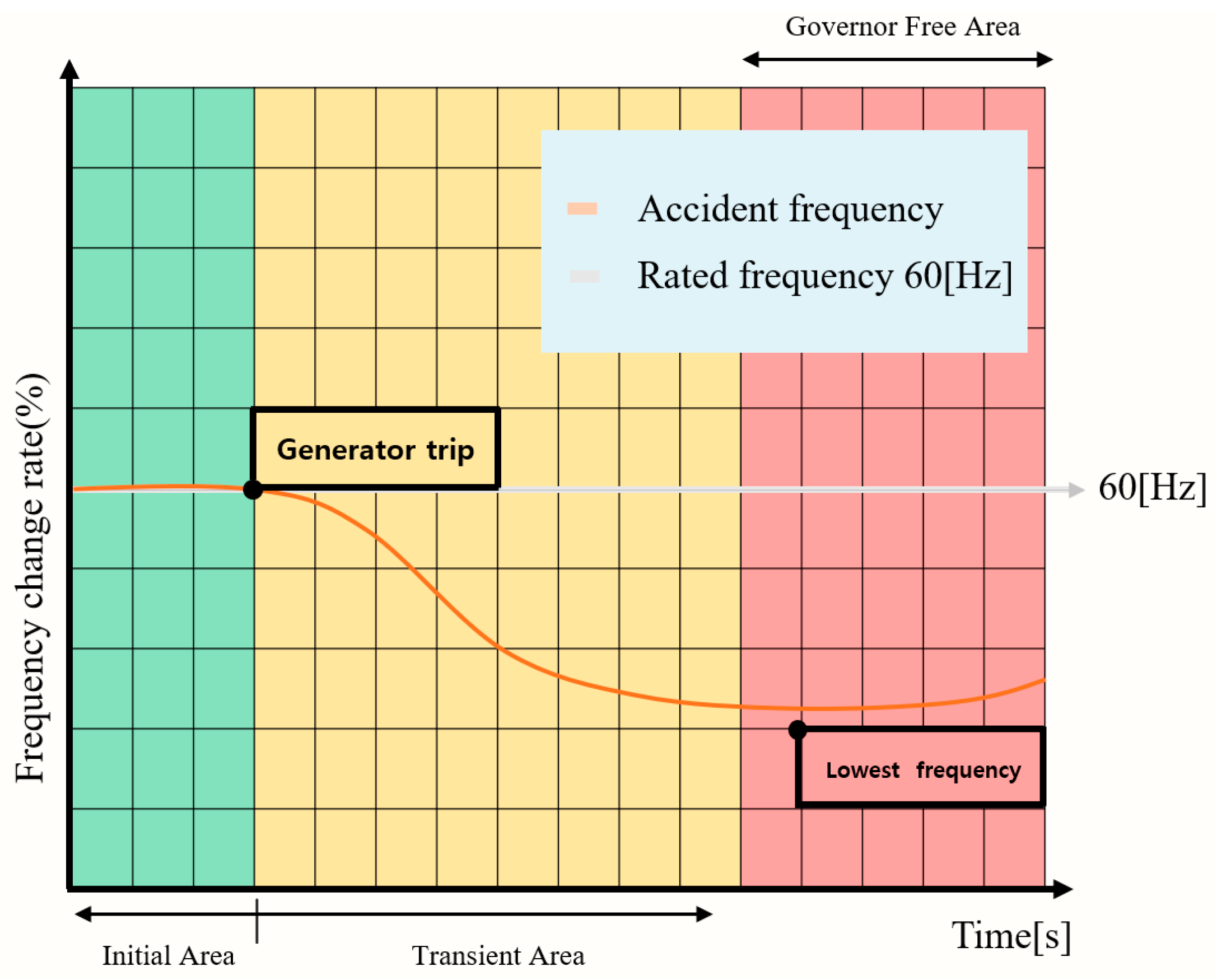
Figure 1 shows the fluctuation in the power system frequency caused by the dropout of a generator in a large-scale power plant. The frequency can be controlled through load and generator inertia, which constitute the preemptive system inertia, as well as the response of the generator governor using a frequency response auxiliary device and automatic generator control (AGC).

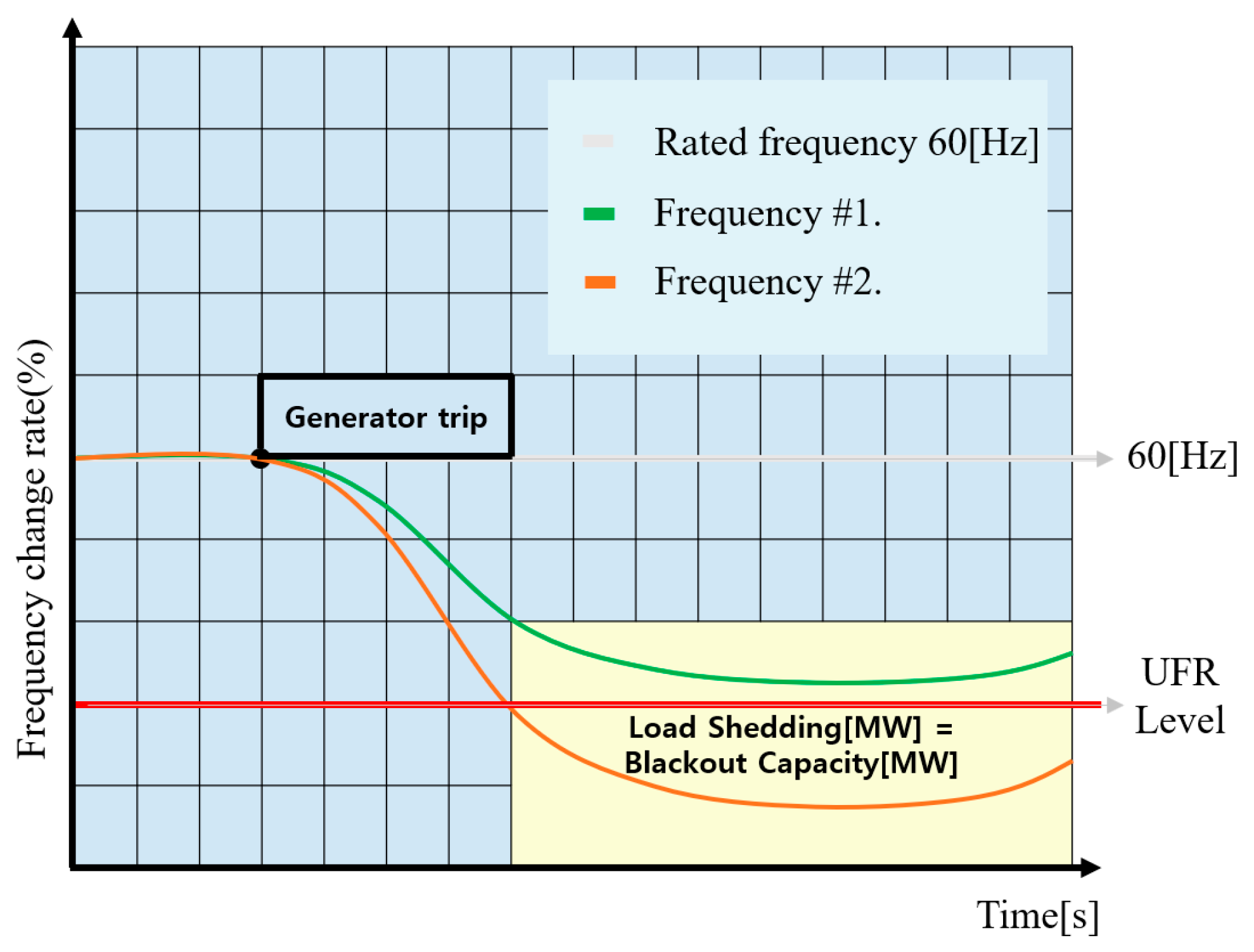
Here, the AGC helps restore the reference frequency to 60 Hz by adjusting the governor of the generator after a disturbance occurs in the system [6]. Figure 2 illustrates how the power system frequency drops to the Under Frequency Relay’s (UFR, red line) first stage level (rated frequency), which is the frequency threshold for domestic grid load shedding.

Load shedding is a system protection protocol that maintains the balance between power supply and demand by inducing a power outage when the frequency of the power system remains at a dangerous level (as indicated by the gray shade in Figure 2) for more than 1 s in order to restore frequency stability [7].

Domestic load shedding was implemented in accordance with the Standards for Power System Reliability and Electric Quality Maintenance [8]. Specifically, a frequency load shedding plan was established to lower the frequency level through Articles 14 and 16 and to prevent deviation from the scope of Chapter 2, Article 4 in the event of a failure.

However, causing a large-scale load outage, as contemplated in the above plan, is one of the measures that a grid operator would most likely try to avoid. Therefore, to prevent such an event, the system operator secures a margin for frequency stability by pre-emptively reducing the power generation of large-scale power generation complexes through generation constraints to maintain the frequency within the safe range indicated by the green line in Figure 2 [9].

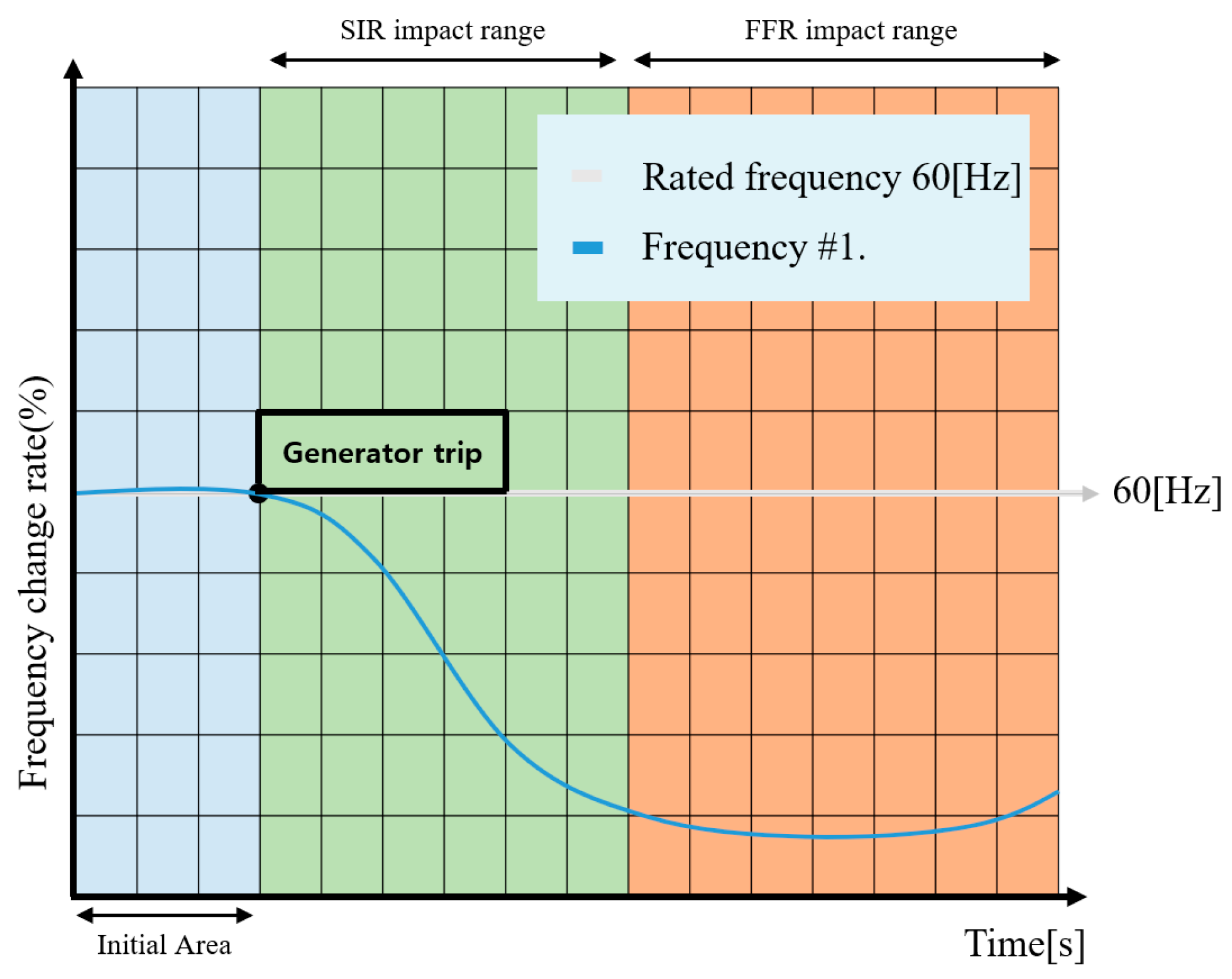
Generally, auxiliary system frequency response facilities, as shown in Figure 3, are classified into Synchronous Inertial Response (SIR) and Fast Frequency Response (FFR) facilities.

SIR facilities are represented by synchronous compensators, which provide a faster and more immediate frequency response than FFR thanks to the use of the natural inertial force of the rotating body. This is included in the inertial force inherent in the system and is similar to preemptive inertia. On the other hand, FFR is achieved through active power output devices that can be utilized within 2 s of the start of the event and can last for at least 8 s. The FFR is represented by ESS (FR-ESS) equipment, which can also respond within 2 s of the occurrence of the event.

FR-ESSs are not rotating machines, but a form of acquired inertia that helps restore the inertia of the generator introduced into the system. This is achieved by injecting active power into the system at once, thereby quickly restoring the balance between the supply and demand [4,10].

In the case of domestic grids, power demand and supply areas are generally divided into metropolitan areas and provinces. Renewable energy sources that facilitate the supply–demand linkage between both regions in anticipation of distributed generation are mostly located in rural areas due to geographical and economic factors, resulting in a growing differentiation between the two regions [11]. To address the challenges arising from the differences between the demand and supply of active power and to ensure system frequency reliability, the Korea Electric Power Corporation (KEPCO) built a 376 MW FR-ESS in 2016 [5,12], which has allowed for savings of about 24 billion KRW in electricity purchase costs to be achieved since it began commercial operation in 2017.

The operation of an FR-ESS is illustrated in Figure 4. Briefly explained, when the frequency exceeds the specified limit, the battery energy storage system (BESS) absorbs active power from the system (BESS charging), thus lowering the frequency. Conversely, when the frequency falls below the specified range, the BESS supplies active power to the system (BESS discharging), which helps maintain the rated frequency and improve the frequency stability of the system.

The renewable energy that flows into the current grid originates from intermittent natural resources and, hence, its output fluctuates. From the perspective of the system operator, the energy output must be constant to ensure stable power system operation. In a traditional system without renewable energy, the supply and demand (frequency) can be properly maintained by accurately estimating load fluctuations.

To address the intermittency of the renewable energy input to the power system, it is necessary to expand the installation of BESSs. By participating in the system operation as FR-ESSs through FR control facilities, BESSs can function as reserve resources.

This study has been deemed to be highly beneficial in achieving stable power system operation and overcoming uncertainty. Its findings can be fully utilized to contribute to frequency stability, provide inertial assistance, ensure stable system operation, and promote the expansion of sustainable renewable energy power generation sources.

When a transmission line failure occurs, an instantaneous imbalance between the supply and demand of active power occurs due to an increase in the transmission line’s transfer impedance. To mitigate this, the FR-ESS is operated to minimize the system frequency drop by compensating for some of the lost active power through simultaneous discharge operation.

In a previous study, Cheung et al. [13] developed an algorithm for evaluating power system transmission loss. In a traditional power system, the power of a transmission line flows naturally in the direction with the smallest transmission loss. Thus, line loss is not a major consideration for electricity market participants. However, as the scale of the system increases and various devices are connected to the grid, the accurate analysis of active power transmission loss becomes a crucial tool for achieving high power transmission efficiency. Cheung’s algorithm accurately calculated the transmission loss of some buses in the power systems of Hong Kong, and Australia contributed to their efficient operation and visualization.

The FR-ESS facility used in this study has certain operational and physical limitations that may prevent it from fully demonstrating its rated output if it is unsuitable for response or installed on an inefficient bus that causes loss in response during significant events. Therefore, the selection procedures and rules for selecting a suitable bus for the FR-ESS need to be studied. In a previous study, Han [14] replaced the self-starting generator used for emergency recovery operations during major blackouts with a BESS, which helped suppress the overvoltage phenomenon caused by the shortening of the city transmission line.

Han proposed two operating modes. Mode #1 is a constant power generation constraint reduction operation mode, and Mode #2 is a BESS operation mode used as a self-starter. Typically, the likelihood of a power outage in all systems is very low. When a self-starting generator is replaced with a BESS, its idle state is used to reduce power generation constraints and analyze the capacity of the optimal BESS from the perspectives of the power conversion system (PCS) and reactive power.

Figure 5 displays a simplified diagram of our power system, which comprises one generator, one load, and four buses. The contingency failure scenario simulated in this study involves the failure of the transmission line connecting buses 2 and 3. Such failure leads to large-scale active power loss, disrupts the supply demand balance due to a decrease in supply capacity, and lowers the frequency.

Based on the system diagram shown in Figure 5, if the transmission line is opened due to an accident, the generation stage and load area are separated, creating an island. In this case, it is impossible to calculate the current as an island since the electrical circuit is in a complete open state. However, since the actual system structure consists of a variety of serial and parallel structures composed of several weak links along the main link, the island situation was not considered in the scenario. Therefore, when a failure occurs and the frequency fluctuates, the FR-ESS that was previously connected to a specific bus monitors the system frequency in real time and performs frequency assistance through the controller when the frequency reaches the pre-established threshold value.

The ability of the system to stabilize frequency with the aid of inertial assistance was evaluated for several buses. The active power sensitivity of each bus was calculated based on the voltage equation and sensitivity matrix used in the current calculation. By comparing and verifying the frequency fluctuations that occur during failure with the provided sensitivity index table, we introduce the process of selecting the optimal bus that contributes the most to frequency stability using only the sensitivity index.

The system analysis program used PSS/E to analyze the system based on the eighth supply and demand plan provided by KEPCO using 2020 data.

The remainder of the paper is structured as follows: In Section 2, we provide the theoretical background for the study, and based on this, we visually display the bus that is judged to have excellent active power absorption. We then derive the frequency increase effect through the sensitivity index. In Section 3, we describe the actual scenario of a frequency drop in the system, conduct a case study, and verify the sensitivity index by reviewing the frequency change generated by the contingency failure scenario. In Section 4, we present the conclusions of the study, discuss the implications of the research results and process, and provide our thoughts on the direction of sustainable development for the proposed sensitivity index.

2. Mathematical Approach to Active Power Sensitivity Index

When the power is generated far from where it is demanded, it must be transmitted to the demand location through transmission lines. Due to the mesh configuration of the system, even if a line with a small power flow fails, the power flow can be redistributed, and the balance between supply and demand can be maintained.

However, the failure of high-current interface lines such as the 765 kV and 345 kV lines can cause a fatal imbalance in the power system. Moreover, if the generator is electrically isolated [15], as shown in Figure 5 and Figure 6, synchronization loss can occur in the synchronous power generation facility due to phase angle stability issues. In the worst-case scenario, a large-scale blackout may occur along with a generator outage.

In Figure 6, our power system comprises an integrated power source, a composite load, and a transformer facility.

This simplified system can be represented by three “bus areas”: the generation, transmission, and load stages. Typically, power flows from the generation to the load area.

The physical distance between buses 1, 2, 3, and 4 can be thought of as the length of the transformer windings and connected conductors. Between buses 2 and 3, a power transmission line occupies most of the length, spanning tens to hundreds of kilometers. This area, physically exposed to the outside, has the highest probability of failure.

Therefore, most facility accidents involving power systems occur in transmission areas. If a line failure occurs at the transmission end, an imbalance in supply and demand occurs. In the worst case, the load may experience a power outage depending on the scale of the accident and the system operating conditions.

If the system is reinforced to prepare for such situations by introducing an FR-ESS, the optimal installation location is the load area, including buses 3 or 4. In particular, bus 4 is the most suitable for FR-ESS installation because it is the closest to the load and can avoid transmission loss of the load in the substation and the transmission line leading to buses #3 and #4. In addition, if the FR-ESS is activated in bus 4, active power can be safely and efficiently supplied to the load even if an accident occurs at the transmission and power generation stages.

However, in an actual system, the physical location of the load cannot be specified, such as load L connected to bus 4, but is scattered throughout the system. Therefore, finding a bus that corresponds to the actual bus 4 is close to impossible. Therefore, as the next-best alternative, this section proposes a mathematical approach to search for buses corresponding to bus 3, considering high grid frequency sensitivity and numerous connected loads. The selection is based on the size of power flowing through each bus. Consequently, the frequency sensitivity indices for all buses in the power system and under each accident scenario were indexed.

Generally, the power flow cannot be arbitrarily controlled due to the natural flow caused by line impedance [11]. Therefore, the key task of this study is to find, among the numerous buses in the system, the bus that most smoothly absorbs active power, with the final goal of estimating the degree of these effects at the static power flow calculation level.

The most effective location for installing an FR-ESS to provide frequency support is a bus with high frequency sensitivity to active power. The degree of sensitivity is determined by considering only the line impedance as the load component that causes the voltage drop, as shown in Figure 7 and Equations (1)–(11) below.

As shown in Figure 7, the power flowing into bus 2 and out of bus 1 can be determined by the line constant, bus voltage, and phase, which are known values for any two arbitrary buses.

The power supplied to buses 1 and 2 can be denoted as transmitted power S₁ and received power S₂, respectively. The relationship between voltage V₁ across bus 1 and voltage V₂ across bus 2 is as follows:

$$V_1=V_2+IZ$$

(1)

Here, the values of $V_1$ and $V_2$ are converted into P.U. units under normal system operating conditions and correspond to Fast Frequency Response (FFR) resources, which are gains generated through a posteriori control. Therefore, after an accident, the droop control unit of the FR-ESS receives and outputs the details of the accident due to a sudden collapse of stability. The system transient state before the output is already close to an unrecoverable level or the voltage level in the FR-ESS installation bus, and nearby buses have V = 0.95~1.05 P.U. If it is outside of this range, the rated output discharge of FR-ESS is impossible according to Equations (4)–(7). Because the voltage collapse causes an unstable state that cannot be recovered, it is difficult to observe a meaningful effect even if the discharge operation is performed in a situation where the voltage stability is lowered.

Typically, the load current, I, is inductive, and the current can be represented as $I^{*}$. The conjugate of the current is taken to determine the phase difference between the voltage and current. In this case, the inductive reactance has a positive value, and the capacitive reactance has a negative value.

Conversely, when taking the conjugate $V^{*}$ of the voltage, the sign is altered and can be interpreted accordingly.

Therefore, the sensitivity index can be calculated assuming that the bus voltage before and after failure is $V_1=V_2$ = 1.0 [P.U.]. According to the power equation, the transmitted power $S_1$ and received power $S_2$ are as follows:

$$S_1=V_1{I}^{*},$$

(2)

$$S_2=V_2{I}^{*}$$

(3)

The current $I^{\mathrm{*}}$ flowing through the transmission line across the buses is expressed by Equation (5) based on Ohm’s law:

$$I^{*}=\frac{V_1\angle {-\theta }_1-V_2\angle -{\theta }_2}{-Z}$$

(4)

Typically, the resistance component of the real part of the line impedance is significantly smaller than that of the imaginary part. Therefore, Equation (4) can be written only in terms of the reactance component $X$:

$${I_x}^{*}=\frac{V_1\angle -{\theta }_1-V_2\angle -{\theta }_2}{-jX}$$

(5)

The transmission end power $S_1$ in Equation (2) can be expressed as follows through the conjugate current:

$$S_1=V_1\angle {\theta }_1·\frac{V_1\angle -{\theta }_1-V_2\angle -{\theta }_2}{-jX},$$

(6)

$$S_1=\frac{{V_1}^2{-V}_1{V}_2\angle {\theta }_1-{\theta }_2}{X}$$

(7)

Here, the active power and reactive power are determined by the real and imaginary parts of the formula. According to the equation, the term containing j corresponds to the real part through the sine component, and the cosine component corresponds to the imaginary part. In this case, the real part represents the active power, while the imaginary part represents the reactive power.

Because the FR-ESS in Equations (2) and (3) is an FFR resource, the voltage before and after an accident is assumed as $V=1.0 \left[P.U.\right].$ Consequently, the magnitude of the current flowing between the buses can be determined based on the reactance and the phase angle difference $\delta ={\theta }_1-{\theta }_2$, resulting in a complex power, as follows:

$$S_1=\frac{{V_1}^2{-V}_1{V}_2\angle \delta }{X}$$

(8)

Through Euler’s formula, the rotating polar coordinate $\delta$ can be represented as a complex number and trigonometric functions. It is transformed as follows:

$$S_1=\frac{{j{V}_1}^2{-j(V}_1{V}_{2}cos\delta +{j V}_1{V}_{2}sin\delta )}{X}$$

(9)

The magnitudes of active power and reactive power flowing into the transmission line and terminals can be expressed as follows. This represents the size accounting for both the load and transmission losses on the supply side.

$$S_1=\frac{V_1{V}_2}{X}sin\delta +\frac{{V_1}^2{-V}_1{V}_{2}cos\delta }{X}$$

(10)

Similarly, the receiving end power can be expressed as follows:

$$S_2=\frac{j\left({ V}_1{V}_{2}cos\delta {-j V}_1{V}_{2}sin\delta \right)-j{V_2}^2}{X} ,$$

(11)

$$S_2=\frac{V_1{V}_2}{X}sin\delta +\frac{{V_1{V}_{2}cos\delta -V_2}^2}{X}.$$

(12)

The frequency increase caused by the FR-ESS discharge only considers the effects of active power supply and demand and the formula for active power, while it excludes the two-term imaginary part corresponding to reactive power. Thus, the active power flowing between the buses in Figure 7 is calculated as follows:

$$P=\frac{V_1{V}_2}{X}sin\delta .$$

(13)

If the changes in voltage and reactance that occur after an accident are ignored, the active power flow can be estimated from the phase difference δ between the buses. As a result, a bus with a larger δ can provide a higher frequency sensitivity.

In the power flow calculation, the relationship between the active and reactive powers can be expressed using the Jacobian matrix, as follows:

$$\left[\begin{array}{c}∆P\\ ∆Q\end{array}\right]=\left[\begin{array}{c}\begin{array}{ccc}\frac{{\partial P}_2}{{\partial \delta }_2}& \cdots & \frac{{\partial P}_2}{{\partial \delta }_n}\\ ⋮& \ddots & ⋮\\ \frac{{\partial P}_n}{{\partial \delta }_2}& \cdots & \frac{{\partial P}_n}{{\partial \delta }_n}\end{array} \begin{array}{ccc}\frac{{\partial P}_2}{{\partial V}_2}& \cdots & \frac{{\partial P}_2}{{\partial V}_n}\\ ⋮& \ddots & ⋮\\ \frac{{\partial P}_n}{{\partial V}_2}& \cdots & \frac{{\partial P}_n}{{\partial V}_n}\end{array} \\ \\ \begin{array}{ccc}\frac{{\partial Q}_2}{{\partial \delta }_2}& \cdots & \frac{{\partial Q}_2}{{\partial \delta }_n}\\ ⋮& \ddots & ⋮\\ \frac{{\partial Q}_n}{{\partial \delta }_2}& \cdots & \frac{{\partial Q}_n}{{\partial \delta }_n}\end{array} \begin{array}{ccc}\frac{{\partial Q}_2}{{\partial V}_2}& \cdots & \frac{{\partial Q}_2}{{\partial V}_n}\\ ⋮& \ddots & ⋮\\ \frac{{\partial Q}_n}{{\partial V}_2}& \cdots & \frac{{\partial Q}_n}{{\partial V}_n}\end{array} \end{array}\right]\left[\begin{array}{c}∆\delta \\ ∆V\end{array}\right].$$

(14)

To briefly introduce the sparse matrix, phase $\delta$, and magnitude $V$ of the voltage, which are known physical properties of the generator bus, load bus, and slack bus, $P$ and $Q$, respectively, are partially differentiated with respect to the active power.

As a result, the effects of $∆P$ and $∆Q$ on $∆\delta$ and $∆V$ can be expressed as a matrix. The sensitivity characteristics of the bus are $\frac{\partial P}{\partial \theta }\gg \frac{\partial P}{\partial V}$ for active power $∆P$ and $\frac{\partial Q}{\partial \theta }\ll \frac{\partial Q}{\partial V}$ for reactive power $∆Q$.

By actively reflecting the above sensitivity characteristics, the complex sparse matrix can be simplified into the following matrix with four sensitivity characteristics:

$$\left[\begin{array}{c}∆P\\ ∆Q\end{array}\right]=\left[\begin{array}{cc}J1& J2\\ J3& J4\end{array}\right]\left[\begin{array}{c}∆\delta \\ ∆V\end{array}\right],$$

(15)

where the constituent $J1$ is $\frac{\partial P}{\partial \delta }$, and $J4$ is $\frac{\partial Q}{\partial V}$. Due to the sensitivity characteristics of the matrix, the change in the reactive power $Q$ is more sensible to fluctuations in the voltage magnitude than in the voltage phase. Conversely, the active power $P$ is more sensible to changes in the voltage phase angle than in the voltage magnitude. Thus, the Jacobian matrix can be expressed as follows:

$$\left[\begin{array}{c}∆P\\ ∆Q\end{array}\right]=\left[\begin{array}{cc}\frac{\partial P}{\partial \delta }& \frac{\partial P}{\partial V}\\ \frac{\partial Q}{\partial \delta }& \frac{\partial Q}{\partial V}\end{array}\right]\left[\begin{array}{c}∆\delta \\ ∆V\end{array}\right].$$

(16)

As derived from the above, in the frequency stability analysis, the effect of the reactive power and bus voltage magnitudes on the result is insignificant, so the change in reactive power can be assumed as $∆Q=0$, and Equation (13) is simplified as follows:

$$\left[\begin{array}{c}∆P\\ 0\end{array}\right]=\left[\begin{array}{cc}\frac{\partial P}{\partial \delta }& \frac{\partial P}{\partial V}\\ \frac{\partial Q}{\partial \delta }& \frac{\partial Q}{\partial V}\end{array}\right]\left[\begin{array}{c}∆\delta \\ ∆V\end{array}\right].$$

(17)

In addition, the FR-ESS only outputs the active power, and the PCS power factor control is not considered in Equation (10) but is expressed as Equation (14). To further simplify the Jacobian sensitivity matrix, it can be expressed in terms of a matrix of susceptance $B$ that represents the degree to which the current flows and replaces part of the sensitivity matrix. Hence, the relationship between the voltage phase and active power is given by the following:

$$\left[∆P_{ij}\right]=\left[B\right]\left[\begin{array}{c}∆\delta \\ ∆V\end{array}\right].$$

(18)

where $i$ and $j$ denote the bus to which the transmission line is connected (i.e., the power drawn from the bus at the receiving end) and the bus at the transmission end, respectively. If a load exists between the two bus lines with only a line loss impedance $Z$, and the voltage drop across the transmission line is uniform, the power observed at the midpoint of the transmission line between buses $i$ and $j$, given ${∆P}_i\approx {∆P}_j$, is as follows:

$${∆P}_{ij}={\sum }_{i=1}^n\left|V_i\right|\left|V_j\right|\left[B_{ij}\left({∆\theta }_i-{∆\theta }_j\right)\right]$$

(19)

According to Equation (14), the change in reactive power is $∆Q=0$, and as mentioned earlier, the reactive power is more sensitive to changes in the voltage magnitude. Therefore, in Equation (16), the minute fluctuation in the active power due to the displacement of the bus voltage is insignificant and, hence, can be ignored. In other words, the magnitude ${∆P}_{ESS}$ of the FR-ESS active power flowing between buses is expressed as

$${∆P}_{ESS}=\sum B \left(\left|{\theta }_F\right|-\left|{\theta }_{ESS}\right|\right).$$

(20)

When a PCS with the same output is secured, the voltage phase ${\theta }_F$ of the fault bus (voltage phase of the bus to which the faulty line is connected in case of line failure) and the phase ${\theta }_{ESS}$ of the bus voltage where the FR-ESS is applied (phase of FR-ESS installation bus voltage) flows in proportion to the phase angle difference $\delta ={\theta }_F-{\theta }_{ESS}$.

If the optimal installation locations for FR-ESS are selected through these results, the actual installed bus ${\theta }_{ESS}$ values for main lines and substations are provided. Through a mutual comparison of the bus frequency sensitivity index $S_{ESS}$ for frequency fluctuations that occur according to failure scenarios, it is possible to predict the frequency rise and its impact. $S_{ESS}$ is ultimately calculated using the following formula:

$$S_{ESS}=\frac{\left|{∆\theta }_F-∆{\theta }_{ESS}\right|}{2\pi }=\frac{\delta }{2\pi }.$$

(21)

The calculated sensitivity index $S_{ESS}$ is verified using case studies in Section 3.

3. Case Study

To select an optimal location for the installation of an FR-ESS, the effects of using different locations must be verified under the same failure scenario.

Various scenarios, such as line ground fault, two-wire ground fault, line-to-line short circuit, three-phase short circuit, one-line dropout, and two-line dropout, produce different types of results; therefore, they must constitute the same accident. Furthermore, it will be easier to understand if it has a form similar to the above failure modes.

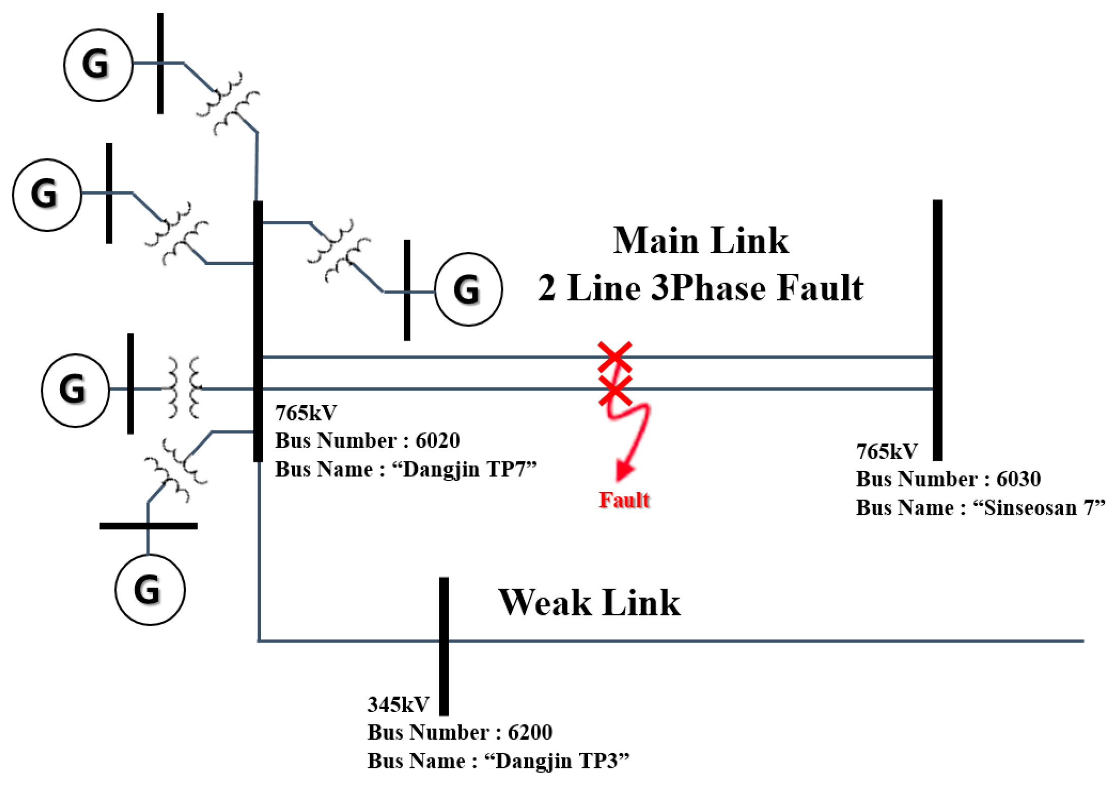
In this section, a two-line contingency failure scenario connecting a 6020 bus (Dangjin TP7 765 kV) and 6030 bus (Sinseosan 7 765 kV) is introduced, as its configuration is the most similar to that shown in Figure 5 and Figure 6.

Figure 8 shows the system diagram elaborated with the power system analysis program PSS/E.

In the system diagram, the 6020 (Dangjin TP7 765 kV) bus is similar to the transmission bus 2 in Figure 6. The 6030 (Sinseosan 7 765 kV) bus, which is connected through two lines, is a receiving bus similar to bus 3 in Figure 6. Several generators are connected to the 6020 (Dangjing TP7 765 kV) bus, corresponding to bus 1 in Figure 6. The 6200 (Dangjing TP3 345 kV) lower bus can be considered as the weak link in Figure 5.

In fact, if the two lines connecting the 6030 (Sinseosan 7) and 6020 (Dangjing TP7) buses, corresponding to the main link in Figure 5 and Figure 6, drop out, all power currents in the area flow to the 6200 (Dangjin TP3) bus, but the large current cannot pass smoothly through the weak link. To express this easily, Figure 8 is an extension of Figure 5 because a weak link cannot smoothly conduct large currents. Figure 9 is also an extension of Figure 5, showing a schematic of the case study scenario of an actual accident based on Figure 5.

Line 2 of the transmission line in the corresponding 765 kV bus scenario was completed in 1998 to transport a maximum power of 6.015 GW generated by the Dangjin thermal power plant, located on the west coast. It is capable of outputting power equivalent to six nuclear power plants. Therefore, in the event of an accident, when the generators of the power generation complex are operating at full load, the phase angle of the generator continuously increases, resulting in an out-of-sync operation risk [13]. To prevent this, the system operator takes protective action, tripping 10 generators when a corresponding line failure occurs with the SPS [15,16,17].

Figure 10 shows the locations of the FR-ESS installations owned and operated by KEPCO. In the next section, based on the 765 kV 2 line drop-out failure scenario, the FR-ESS connected to the bus in Figure 10 is input individually, and the sensitivity index calculated through the output frequency is reviewed.

To verify the sensitivity index under more diverse accidents, we selected two additional contingency failure scenarios and performed three contingency failure analyses. Scenario 1 involved a two-line dropout connecting the 6020 (Dangjin TP7) and 6030 (Sinseosan 7) buses. This scenario represents the main western power transmission line connecting the west coast and the metropolitan area, which is the primary focus of this study. Scenario 2 involved the dropout of the second line connecting the 4010 (Sinanseong) and 1020 (Shingapyeong7) buses, which are responsible for power transportation in the eastern part of the metropolitan area. Scenario 3 involved a line connecting the 8010 (N. Gyeongnam7) and 9010 (Singori7) buses, which was additionally selected to examine the impact on the sensitivity index in Gyeongnam and Busan, which are relatively far from the metropolitan area.

The domestic FR-ESS installations are located at the same location, as shown on the left side of Figure 10a, and are connected to the 154 kV substation in the form shown on the right side of Figure 10b. The degree of frequency change is reviewed according to the FR-ESS installation location. The ESS model uses the “CBEST” model provided by PSS/E, which is described in the PSS/E 33.0 Power Operation Manual [17,18]. The model provides charging and discharging conditions and a comprehensive efficiency model for the PCS and batteries [19]. However, since this study is only interested in frequency control, only the output of the FR-ESS, that is, the PCS, is controlled. The resulting ESS model controls the frequency droop monitors $\frac{df}{dt}$ (rate of change of frequency), discharges when the slope is negative, and charges the ESS when the slope is positive. However, in this study, since only the degree of frequency drop is analyzed, operation control is omitted in the positive slope.

Additionally, we would like to introduce the detailed model, CBEST. The auxiliary controller of the battery model, CBEST, uses the CHAAUT model, which serves as an active power output signal generator. As this control component is not included in the CBEST model, it was compiled using the CONEC command in PSS/E and then input [20].

In this study, considering that the dynamic model parameters for the 13 FR-ESS units to be discussed may vary depending on the manufacturer, all dynamic model parameters for FR-ESS were applied using the parameters provided in the EPRI [21] report. Here, since there is no need to perform reactive power control according to Equations (12)–(15), the reactive power gain was changed to 0.0. As a result, the FR-ESS responds only to frequency and does not track line voltage.

The grid voltage fluctuates in response to the balance between the reactive power supply and demand, and the voltage fluctuation is localized by the reactance X component of the grid; therefore, it has different sizes depending on the measurement point.

In the case of frequency, when the balance between the power supply and demand is broken because the power consumption is greater than the total generated power, the frequency decreases. Conversely, when the generated power is greater than the consumed power, the frequency increases. The frequency fluctuates owing to the influence of the supply and demand of the entire system, resulting in a similar value for all buses of the power system. Therefore, the frequencies measured simultaneously were similar, regardless of the point of observation in the system. Taking this into account, the bus selected for frequency observation under all scenarios was 4600 (Seo Seoul 3 345 kV), and the overall sensitivity table was composed based on this.

Table 1. Sensitivity index and result review table for Scenario 1.

Bus Name Number	${\mathit{S}}_{\mathit{E}\mathit{S}\mathit{S}}$	${\mathit{E}\mathit{S}\mathit{S}}_{\mathit{C}\mathit{a}\mathit{p}}$ [MW]	$∆\mathit{F}$[%]	${\mathit{T}}_{\mathit{t}\mathit{a}\mathit{r}\mathit{g}\mathit{e}\mathit{t}}$ [s]
Sinyongin 4710	0.04314	24	6.1	8.642862
Seoanseong 4310	0.02706	28	6.3	8.642862
Sinchungju 4920	0.04600	16	5.9	8.645863
Singyeryong 6710	0.04769	24	6.1	8.641861
Gimje 6575	0.06353	48	6.7	8.641861
Singimje 6460	0.04681	24	6.1	8.643862
Sinhwasun 7510	0.05525	24	6.1	8.643862
Sogcho 5970	0.06227	24	6.4	8.643862
Nongong 8830	0.06219	36	6.5	8.640861
Gyeongsan 8380	0.04769	48	6.6	8.640861
Ulju 8260	0.03714	24	6.0	8.642862
Ulsan 9830	0.05264	32	6.2	8.640861
Uilyeong 10,310	0.04853	24	6.1	8.641861

lists the sensitivity indices obtained under contingency failure Scenario 1. The following is a detailed explanation:

In Table 1, $S_{ESS}$ is the active power sensitivity corresponding to the indicated bus name, and it is calculated based on Equation (18).

That is, $S_{ESS}$ represents the degree of frequency increase for each bus on the left side of Figure 9 under the two-line contingency failure connecting buses 6020 (Dangjin TP7) and 6030 (Sinseosan 7). The closer $S_{ESS}$ is to 1, the better the frequency-raising effect. ${ESS}_{Cap}$ is the rated output of the FR-ESS, and $∆F$ is the reference frequency of the scenario. The FR-ESS is applied to all buses from the 4710 (Sinyongin) bus to the 10310 (Uilyeong) bus in Table 1. It expresses the effect of frequency variation on the event that occurs as a percentage. When calculating the frequency fluctuation $∆F$, the time at which the lowest frequency occurs is different depending on the bus in which the FR-ESS is applied. Therefore, $T_{target}$ is the point at which the lowest frequency is confirmed (t-axis = x-axis in all graphs), which is the point at which $∆F$ is calculated.

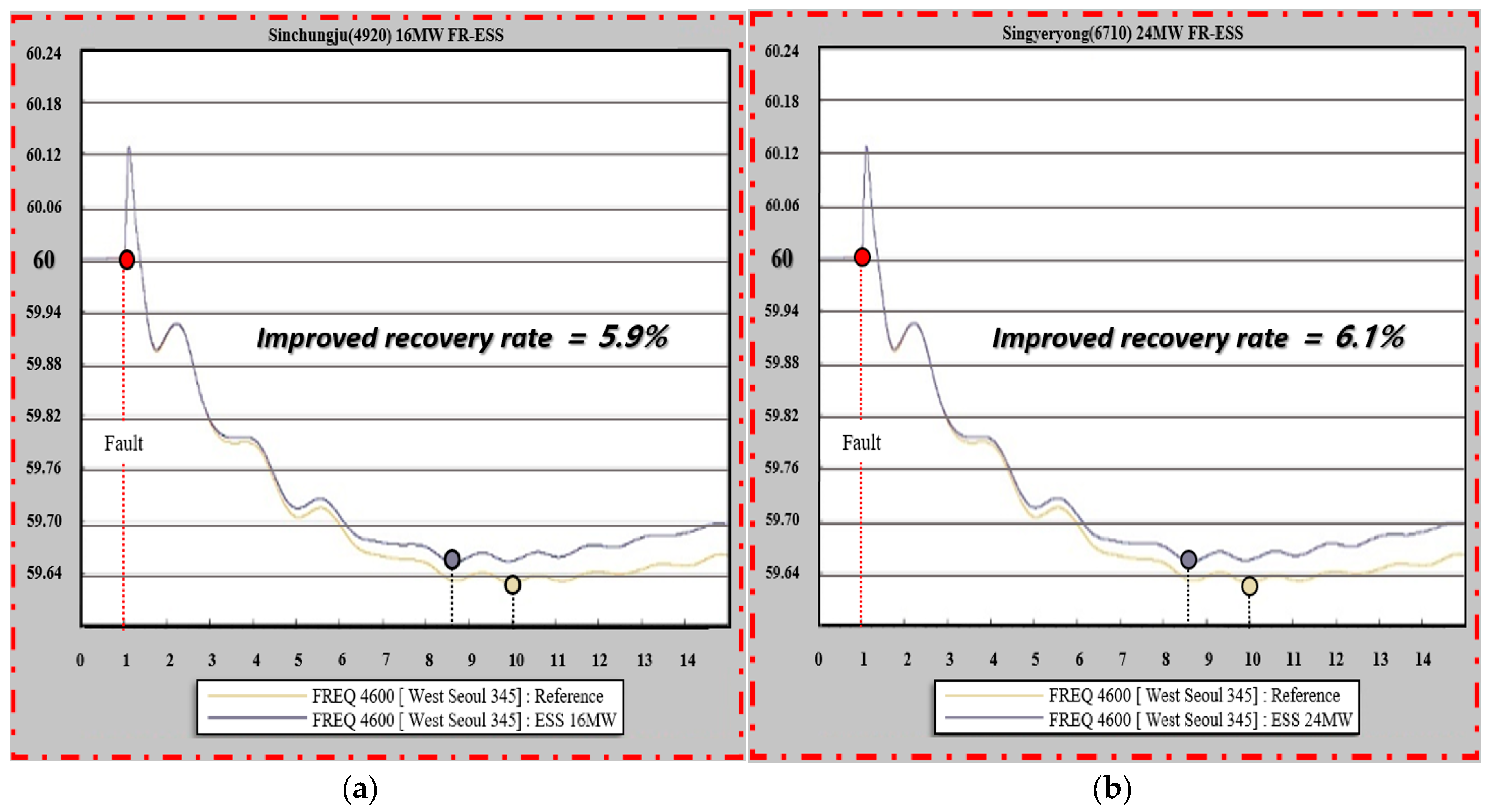
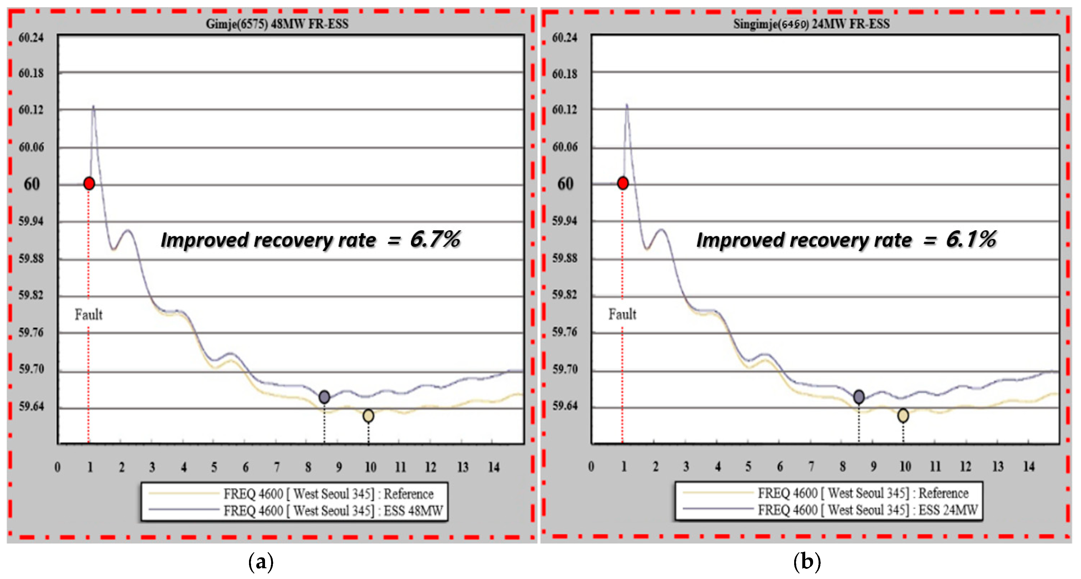
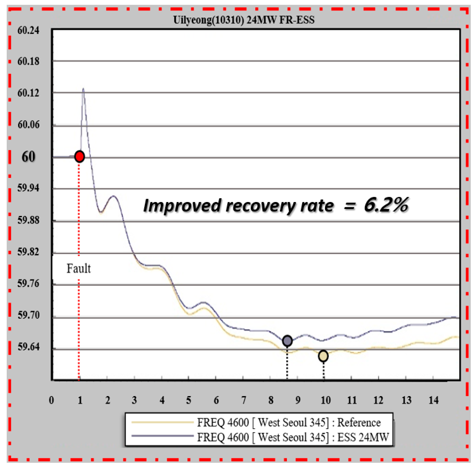
Consequently, if the ${ESS}_{Cap}$ of the BESS is the same, the degree of frequency increase of the bus with a large $S_{ESS}$ is superior than that of the bus without it, and if the frequency fluctuation rate $∆F$ calculated as a result of the review shows the same characteristics, it can be regarded as an ideal research result. The results in Table 1 are shown in Figure 11, Figure 12, Figure 13, Figure 14, Figure 15 and Figure 16.

This allows for the calculation of the $S_{ESS}$ sensitivity for all transmission lines for a given fault scenario. However, since this metric is calculated solely from the perspective of active power, errors can occur in terms of the voltage and reactive power [14,15].

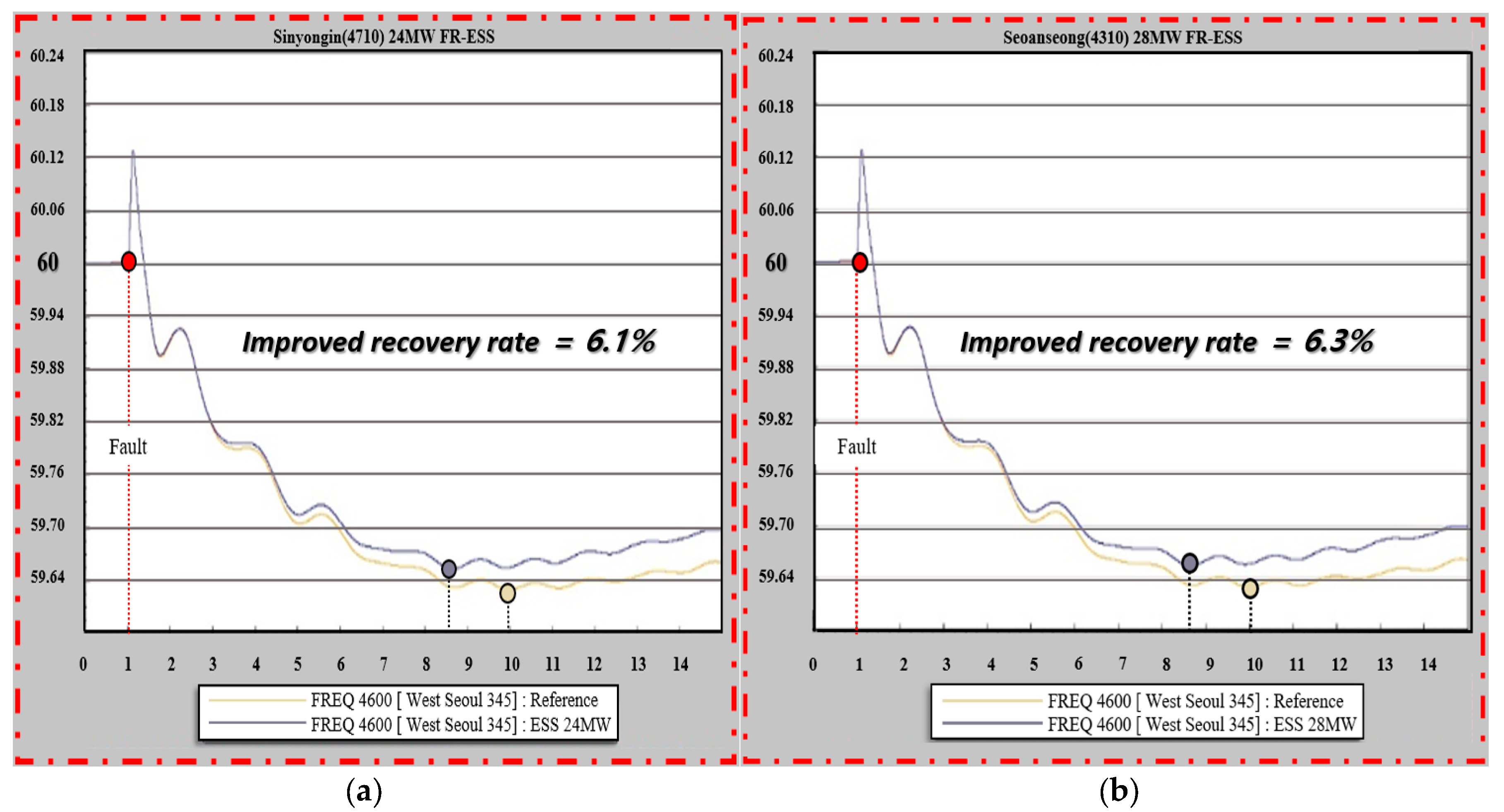
A notable discrepancy can be observed in Table 1 at the 4710 (Sinyongin) and 4310 (Sinseosan) buses. Despite their ESS capacities being nearly identical, it was found that the frequency recovery capability of the 4710 (Sinyongin) bus, with a higher $S_{ESS}$ index, is 0.2% lower. This discrepancy is attributed to its impact on voltage. Currently, the 4710 (Sinyongin) bus is in close proximity to the fault area, and the regional voltage drop could have influenced it. This underscores the inherent limitations in the observability of sensitivity indices.

However, if a wide range of hypothetical faults in the system are considered, and their $S_{ESS}$ indices are calculated as shown in

Table 2. Sensitivity index and result review table for scenarios.

Bus Name Number	${∆}_{\mathit{E}\mathit{S}\mathit{S}}$ (BusNum)	${\mathit{E}\mathit{S}\mathit{S}}_{\mathit{C}\mathit{a}\mathit{p}}$ (MW)	6020-6030 Scenario 1	6030-4010 Scenario 2	8010-9010 Scenario 3
Sinyongin	4710	24	0.04314	0.031944	0.023361
Seoanseong	4310	28	0.02706	0.015861	0.007278
Sinchungju	4920	16	0.04600	0.034806	0.026222
Singyeryong	6710	24	0.04769	0.036500	0.027917
Gimje	6575	48	0.06353	0.052306	0.043722
Singimje	6460	24	0.04681	0.035611	0.027028
Sinhwasun	7510	24	0.05525	0.04411	0.035528
Sogcho	5970	24	0.06227	0.073220	0.081810
Nongong	8830	36	0.06219	0.051139	0.042556
Gyeongsan	8380	48	0.04769	0.036694	0.028111
Ulju	8260	24	0.03714	0.026000	0.017417
Ulsan	9830	32	0.05264	0.041500	0.032917
Uilyeong	10,310	24	0.04853	0.037417	0.028833

, determining the installation location for FR-ESS as the area with the highest average $S_{ESS}$ among them, then it is anticipated that it could be a flexible and deployable FR-ESS installation location for almost all faults.

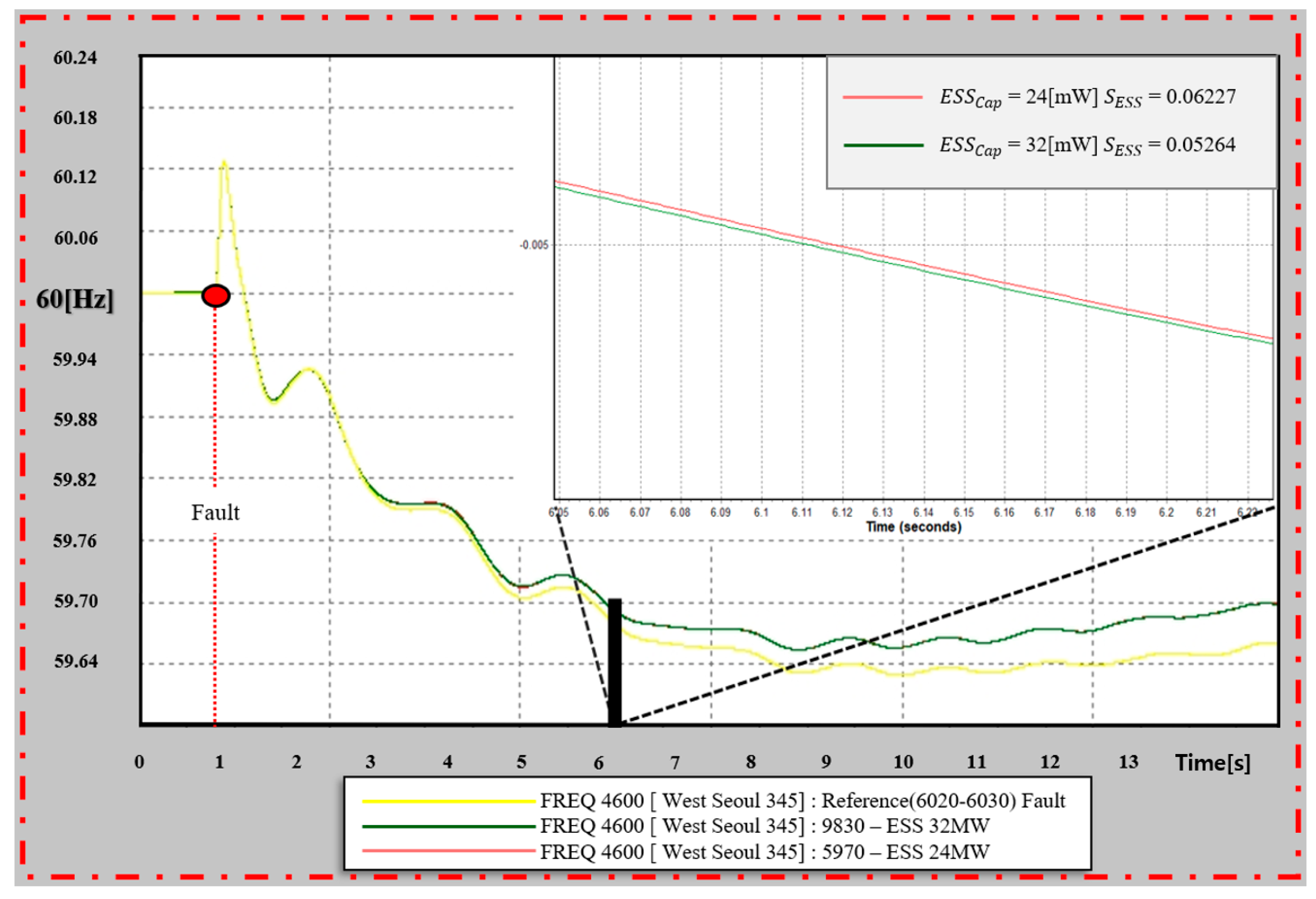
Figure 17 shows an example of the detailed analysis during the simulation. The x-axis of the graph is 60 Hz based on 0, which indicates the rate of change in frequency (i.e., 0 = 60 Hz), and yellow is the reference frequency. The reference represents the result of an accident in the case of no FR-ESS, and the frequency is the lowest because it does not assist in frequency recovery after an accident. The graphs in red (5970 (Sogcho)) and green (9830 (Ulsan)) express the purpose of this study. Here, red has a 24 MW output, and green has a 32 MW output.

However, in the case of red, the sensitivity of $S_{ESS}$ was 0.06627, and in the case of green, $S_{ESS}$ was 0.05264. The output of the FR-ESS connected to the green graph (9830 (Ulsan) bus) is 32 MW, which is approximately 8 MW higher than the 24 MW of the red graph (5970 (Sogcho) bus) in the comparison group. However, according to the sensitivity index, the red (5970 (Sogcho) bus) bar exhibited excellent sensitivity.

Frequency sensitivity. If a sensitivity table is created for the entire bus of the system, the $S_{ESS}$ index should be considered sufficiently when incorporating facilities related to the active power output, such as the FR-ESS, into the system. The above analysis method was applied equally to Figure 17, Figure 18 and Figure 19 below.

Table 2 shows the frequency $S_{ESS}$ sensitivity review results for additional domestic 765 kV lines.

Here, $∆$ESS is the installation location of the FR-ESS, and it is the same as the bus number. Here, $∆{\theta }_{ESS}$ is the value measured at the installation location of the FR-ESS and follows the bus number.

In Table 2, for the sensitivity calculation, the bus lines compared with the 6030 (Sinseosan7), 4010 (Sinansung7), and 9010 (Singori7) buses were specified at the back of the scenario.

The table shows that the buses showing the highest effect on the FR-ESS response in the contingency failure of the 6020 (DanginTP7) and 6030 (Sinseosan7) buses are as follows: the 6575 (Gimje) bus with SESS = 0.0635, according to Scenario 2, can be expected as the 5970 (Sogcho) bus with SESS = 0.0732, according to Scenario 3, is the 6575 (Gimje) bus with SESS = 0.0138. Depending on the scenario, the $∆{\theta }_F$ fluctuates, which, in turn, causes a change in sensitivity.

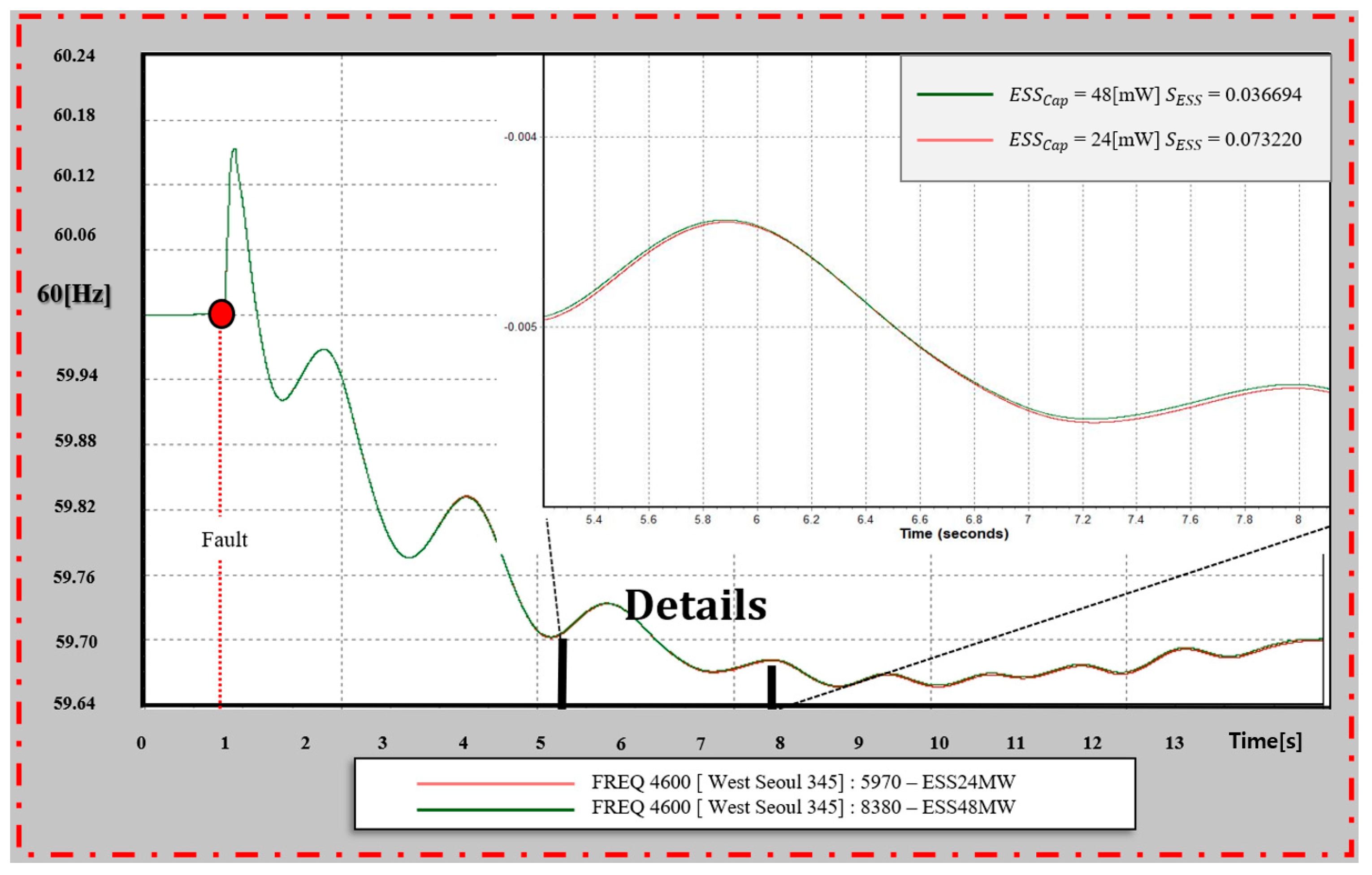
Figure 19 presents a graph of the frequencies of the 5970 (Sogcho) and 8380 (Gyeongsan) buses according to Scenario 2. The reason for introducing the results for the parent ship is that it most effectively represents the purpose and results of this study, as shown in Figure 18. The 5970 (Sogcho) bus has the highest sensitivity among the scenarios in this paper, with $S_{ESS}=$ 0.07322. The sensitivity index of the comparison bus, 8380 (Gyeongsan), is $S_{ESS}=0.036694$, which is located in the lower range of the frequency sensitivity of the scenario. The frequency increase effect of the two buses was superior to that of the 8380 (Gyeongsan) bus, with a very slight difference, as shown in Figure 19.

However, the rated output of the two has a difference of about two times, and if we compare the results of the FR-ESS output Table 2, it is evident that this result is not an insignificant difference. The results showed a significant encouraging effect. Interpreting this in the opposite way, if the installation location of the 24 MW FR-ESS is well selected through the sensitivity index $S_{ESS}$, it can have almost an equivalent performance to the 48 MW class FR-ESS, corresponding to 200%.

The review of Scenario 1 is omitted because it was replaced, as shown in Figure 16. Presumed failure Scenario 3 is further reviewed in the same manner as above.

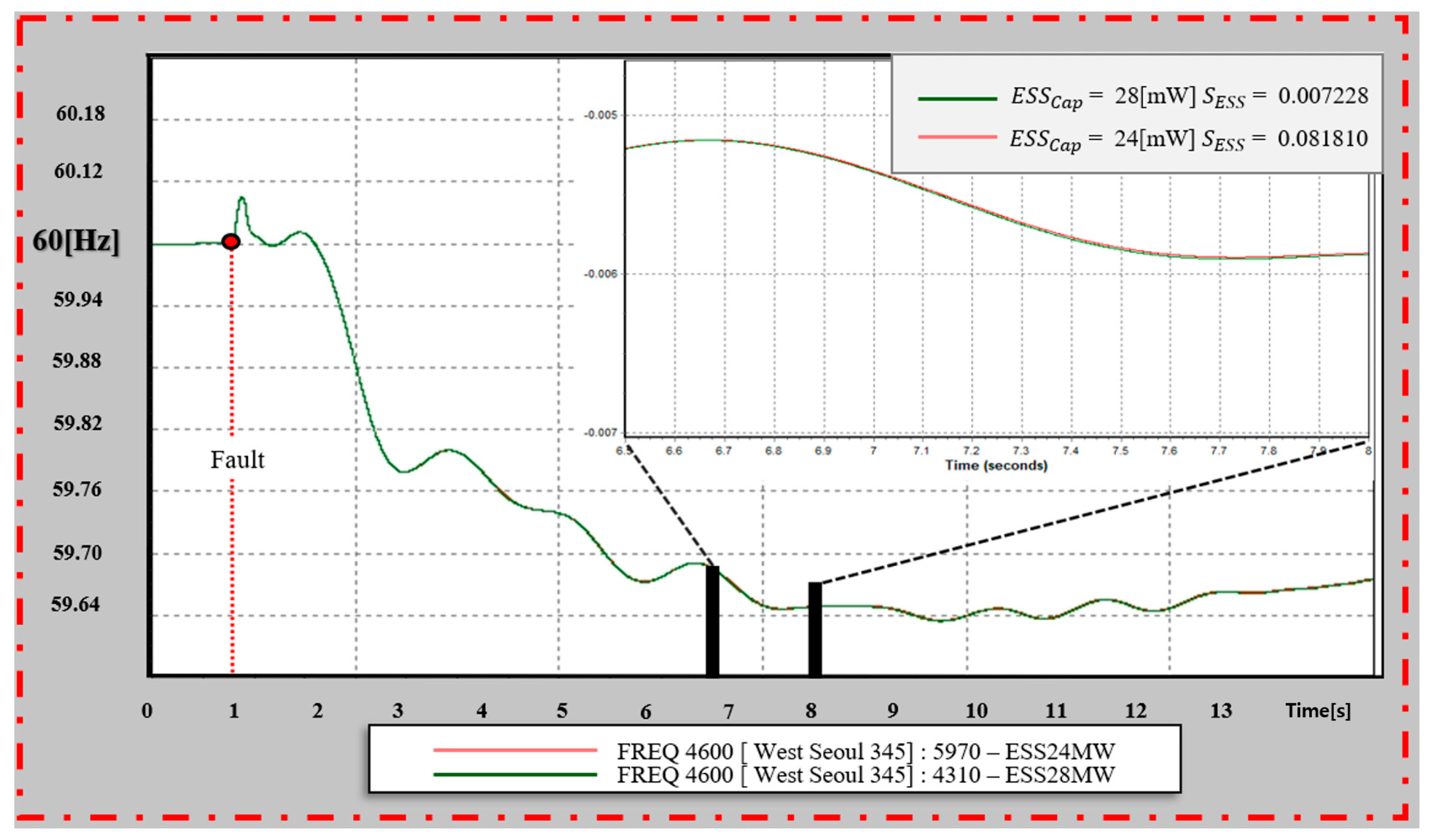
Figure 20 is the frequency review result for scenario 3. This scenario is a contingency failure of the 765 kV line 1 connecting the 8010 (N.Gyeongnam7) bus and the 9010 (Singori7) bus. An additional frequency review was performed because it was a failure in a location far from the metropolitan area. Among the scenario results, the frequency change results of the 5970 (Sogcho) and 4310 (Seoansung) motherships are cited.

Through Table 2, it can be confirmed that the 5970 (Sogcho) bus has a high sensitivity with S = 0.08181, and the 4310 (Seoansung) bus has a low sensitivity with S = 0.02811.

In the case of the 5970 (Sogcho) bus, the output is approximately 15% smaller than that of the 4310 (Seoansung) bus; however, it shows a higher frequency increase rate of accidents.

In this section, three failure scenarios are analyzed based on the frequency stability. If the table provided in Table 2 is fully utilized, it is necessary to fully consider the index when feeding facilities related to active power as well as the FR-ESS to the system. For example, in the case shown in Figure 17, if a 24 MW FR-ESS is replaced with a simple PV, it is possible to secure the same level of frequency stability as a PV with an output of 48 MW.

4. Conclusions

This study examines the optimal location for the installation of an FR-ESS for frequency control. Using the basic power flow formula, the power magnitude across a bus can be determined from the voltage magnitude and phase angle. In this study, an active power sensitivity index, $S_{ESS}$, was developed to predict the change in the bus unit frequency when a contingency failure occurs. This was carried out using the Jacobian and sensitivity matrices used for power flow calculations. To verify the proposed index, three contingency failure scenarios were analyzed on a 765 kV transmission line connecting six different buses, namely, 6020 (DangjinTP7), 6030 (Sinseosan7), 4010 (Shinanseong7), 1020 (Shingapyeong7), 8010 (NorthGyeongnam7), and 9010 (Singori). An intentional system frequency drop was induced by applying these scenarios to the eighth supply and demand plan. The condition for excellent sensitivity was identified as the situation where $S_{ESS}$ is closest to 1, that is, $S_{ESS}\cong 1$. The frequency sensitivity index $S_{ESS}$ was then calculated for buses with ESS installed, finding many buses with poor active power outputs but better frequency recovery abilities. In particular, Scenario 2 demonstrated that a 24 MW FR-ESS connected to a high-sensitivity bus had a higher frequency recovery performance than a 48 MW FR-ESS with relatively low sensitivity. Consequently, the validity of the sensitivity index $S_{ESS}$ was confirmed, providing it with an encouraging effect for follow-up studies.

However, through a review of the results in Figure 17, Figure 18 and Figure 19 and Table 1 and Table 2, the limitations of this study were identified, along with potential areas for improvement in future studies.

First, the proposed $S_{ESS}$ involves a very theoretical approach that disregards various factors that become relevant when an actual MW-class FR-ESS is incorporated into the system, such as the capacity of the substation transformer, overload of the lines near the FR-ESS response bus, operational constraints caused by the system situation and environment, and geographical features like the location and installation area.

Second, the study neglected the quantitative characteristics of the sensitivity index, which could compromise its reliability. Here, we have two buses with sensitivities of $S_{ESS}$ = 0.05 and $S_{ESS}$= 0.1. In such a case, the current sensitivity index cannot quantitatively determine the degree of frequency gain of the two buses. Although the sensitivity table predicts that the bus with $S_{ESS}$ = 0.1 will have a better frequency-raising effect than the one with $S_{ESS}$ = 0.05, estimating the degree of the effect remains challenging. Therefore, it is necessary to improve the sensitivity index to quantitatively determine this effect.

Third, the omission of $∆Q$ from the sensitivity index is a concern. The $S_{ESS}$ was calculated in terms of extremely active power. However, the fluctuation of $∆P$, which is composed of the Jacobian sensitivity matrix of the tidal current calculation, affects the partial derivative $(\partial$) component, $∆V$, while its size is insignificant compared to $∆\delta$. Thus, the existence of $∆P$ clearly introduces a potential for error in calculating the $S_{ESS}$ sensitivity.

Finally, new technology facilities, such as flexible AC transmission system (FACTS) facilities, Back-to-Back (BTB) systems, and inertial auxiliary synchronous ancestors, which are currently being used in many power systems, define reactive power as their main control target. Therefore, analytical techniques that examine the effects of components on active power and frequency must be further advanced compared to traditional techniques.

Keeping the above in mind, in a follow-up study, we intend to develop a sustainable sensitivity $S_{ESS}$ model that takes into account factors such as renewable energy, inertia, new power facilities, and reactive power.