Abstract
Accurate online parameter identification and state of charge (SOC) estimation are both very crucial for ensuring the operating safety of lithium-ion batteries and usually the former is a base of the latter. To achieve accurate and stable SOC estimation results, this paper proposes a model-based method, which incorporates a vector forgetting factor least square (VFFLS) algorithm and an improved adaptive cubature Kalman filter (IACKF). Firstly, considering it is difficult for the traditional forgetting factor recursive least square (FFRLS) algorithm to balance the accuracy, convergence, and stability for multiple parameters with different time-varying periods, an improved VFFLS method is employed to determine the multiple parameters of the first-order RC battery model online. It supersedes the single forgetting factor in the FFRLS with multiple forgetting factors in a vector form for improving adaptive capability to multiple time-varying parameters. Secondly, aiming at the fact that the standard cubature Kalman filter (CKF) cannot operate properly when the error covariance matrix is non-positive definite, which is caused by disturbance, initial error, and the limit of the computer word length, the UR decomposition rather than the Cholesky decomposition is applied, thus improving the algorithm stability. In addition, an adaptive update strategy is added to the CKF to enhance accuracy and convergence speed. Finally, comparative experiments with different operating patterns, positive and non-positive definite error covariance matrices, and temperatures are carried out. Experimental results showed that the proposed method can estimate the SOC accurately and stably.
1. Introduction
With the increasing energy crisis and environmental pollution, new/clean/renewable energy power generation such as nuclear power, water power, wind power, and solar power have been rapidly developed around the world in the last decades [1,2]. In addition, electric vehicles (EVs) have been widely used in both industry and academia communities for reducing the emission of greenhouse gases [3,4,5]. The energy storage system (ESS) is a key component of EVs. Lithium-ion batteries (LIBs) are known to have high energy capacity, high columbic rate, no memory effect, and long cycle life, so they have been commonly used as the ESS of EVs [6,7,8]. LIBs are subjected to significant nonlinearity and dynamics. Thus, in order to ensure the operating safety of the LIBs, an effective battery management system (BMS) is required to monitor battery parameters and states, such as state of charge (SOC), state of energy (SOE), and state of health (SOH) [9,10,11]. Among these states, SOC, indicating the current capacity state of the LIBs, is an important index for avoiding abnormal charging/discharging of the LIBs. However, SOC cannot be acquired directly using a sensor, so it is often estimated based on other measurable parameters, including voltage, current, and temperature. Additionally, the accuracy of SOC estimation is influenced nonlinearly by many factors such as model error, current rate, ambient temperature, battery degradation, and cell inconsistency [12,13]. Consequently, the quick and accurate estimation of battery SOC is still an open and challenging issue.
Currently, a large number of methods have been put forward for SOC estimation. In general, they can be divided into four categories: the Coulomb counting (CC) method [14], the open-circuit voltage (OCV) method [15], model-based methods, and data-driven methods. The CC method is commonly used in real-world applications because of its easy implementation, simple calculation, and low cost. However, as an open-loop method, it is highly dependent on the accuracy of the current sensor and requires an accurate initial SOC value [16]. The OCV method calculates the SOC based on a nonlinear OCV–SOC relationship, which is usually stored in a lookup table. Accurate measurement of the OCV can accurately estimate the SOC. Nevertheless, it requires a long time to measure the OCV, thus the OCV method is unsuitable for online estimation [17]. The data-driven methods do not require the assumption of an explicit battery model and, accordingly, they are becoming increasingly popular [18]. Commonly used data-driven methods include artificial neural networks [19], support vector machines [20], and fuzzy logic [21,22]. The data-driven methods can learn a nonlinear mapping model between the SOC and measured data such as voltage, current, and temperature, and they do not require extensive domain knowledge about the LIBs [23,24]. However, the data-driven approaches are still limited by factors including the small simple data, tedious feature extraction, huge computational cost, and strong dependency on battery operation conditions [25].
In contrast, the model-based methods are more suitable for online use in actual conditions because of their reasonable trade-off abilities among accuracy, complexity, and computation load [26]. The process of a model-based method generally involves three steps: battery modeling, parameter identification, and algorithm implementation.
Electrochemical models (ECMs) [27,28] and electrical equivalent circuit models (EECMs) [29,30,31] are the two most commonly used battery models. Compared to the ECMs, the EECMs have lower complexity and higher compatibility, so they are more favorable for online SOC estimation with embedded systems. EECMs mainly include three categories: the Rint model [29], the Randles model [30], and the nRC models [31]. Among them, the first-order and second-order RC models are the most widely used because they give good consideration to both accuracy and complexity. After selecting an appropriate model, the model parameters need to be further determined.
The accuracy of battery model parameter identification has a high impact on the precision of SOC estimation. The parameters of EECMs can be identified offline or online. However, due to the high sensitivity of the battery parameters to the depth of charging/discharging, current profiles, and battery aging levels [32], the offline method may cause errors in actual working conditions. As a result, the recursive least square (RLS) family has been commonly used to identify battery model parameters online [33]. However, it is challenging for the classical RLS algorithm to meet both the accuracy requirement and the short-term memory capability, and with the increasing amount of observation data, the time variability becomes worse and even leads to data saturation [34]. In contrast, the FFRLS method can strengthen the influence of new data but weaken the contribution of history data to the current identification result by introducing a forgetting factor, maintaining a fast convergence rate, and a high storage capability for long-term data. Nevertheless, the FFRLS easily experiences abnormal fluctuations and even divergence under complex working conditions [35]. Furthermore, the model parameters to be identified change at different rates when the battery is in operation. Hence, it is not recommended to identify multiple parameters changing at different rates [36] by using a single forgetting factor and, accordingly, some improved FFRLS methods have been proposed to address this issue [37,38]. For example, the authors of [38] proposed a vector forgetting factor least square (VFFLS) algorithm to identify the parameters of different battery types on the basis of fully reducing the complexity of the identification process. It employs a set of forgetting factors rather than a single forgetting factor to improve adaptive capability to multiple time-varying parameters with different time scales simultaneously. This feature makes it favorable for EV applications, where battery model parameters such as open circuit voltage, ohmic resistance, and polarization resistance/capacitance vary at different rates [39].
In terms of estimation algorithms, the most widely used methods are Kalman filters, including the extended Kalman filter (EKF), unscented Kalman filter (UKF), cubature Kalman filter (CKF), etc. [40,41]. Among them, the CKF, first proposed in 2009 by Arasaratnam and Haykin [42], has high fitting accuracy, especially for high-order nonlinear systems, which is conducive to achieving high-precision battery SOC estimation. The Cholesky decomposition used in the UKF and CKF requires the matrix to be symmetric positive definite. However, the rounding and discretization in hardware calculation may cause a cumulative error. Then, the covariance matrix may not always be symmetric and positive definite, further resulting in filter divergence [43]. To address this problem, scholars have proposed some improved algorithms. Zhang et al. [25] used the singular value decomposition (SVD) as a substitute for the Cholesky decomposition in the conventional AUKF to realize robust SOC estimation. Wang et al. [44] proposed a combined method, which incorporates the alternative generalized least square method with the forgetting factor and the robust H∞-CKF based on singular value decomposition for SOC estimation of LIBs. Li et al. [45] combined an adaptive cubature Kalman filter (ACKF) using Frobenius-norm-based QR decomposition and an H-infinity filter to estimate the battery SOC. Tian et al. [46] compared and analyzed the differences in the performance of the CKF algorithm caused by using SVD, UR, and LU decomposition instead of Cholesky decomposition. The results showed that all three matrix decomposition strategies can avoid filter failure caused by the non-positive definiteness of the error covariance matrix, and in general, the UR decomposition outperformed the other two methods, showing moderate convergence speed and computational cost, and it is robust against the initial value of the error covariance matrix.
This paper proposes an approach that incorporates a multi-forgetting factor recursive least square algorithm and an improved adaptive cubature Kalman filter for online estimating of the model parameters and SOC of LIBs. The VFFLS algorithm is used for model parameter identification, which replaces the single forgetting factor in the classical FFRLS with multiple forgetting factors, so as to deal with the issue that it is difficult for the traditional FFRLS algorithm to make a trade-off among accuracy, convergence rate, and stability of parameter identification. The UR decomposition is introduced to be a substitute for the Cholesky decomposition used in the traditional CKF so that the filter can always work well no matter whether the error covariance matrix is positive or non-positive definite. To assess the efficacy of the proposed method comprehensively, experiments are carried out under a set of typical driving cycles and temperatures with both positive and non-positive definite error covariance matrices. The proposed method provides an effective solution for online estimating of battery model parameters and SOC under highly dynamic operating conditions.
The remainder of this paper is structured as follows: Section 2 introduces the battery equivalent circuit model and the parameter identification method. Section 3 details the improved ACKF algorithm based on UR decomposition for SOC estimation. Section 4 introduces the experimental setup. Section 5 presents the experimental results and discussion. Finally, the paper is concluded in Section 6.
2. Battery Model and Parameters Identification
2.1. Battery Model
In order to realize SOC estimation using the Kalman filter algorithms, an EECM is requisite. Since the first-order RC model can reconcile the accuracy and efficiency, revealing superiority over other EECMs [47], it is applied to simulate the battery dynamic behaviors in this paper. The first-order EECM is illustrated in Figure 1, where Uoc stands for open circuit voltage, Rp and Cp are polarization resistance and capacitance, respectively, Ro is ohmic resistance, IL indicates load current, and Ut represents terminal voltage. In this paper, load current, IL, is supposed to be positive during discharging and negative during charging.
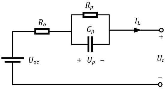
Figure 1.
The first-order RC battery model.
Based on Kirchhoff’s law and the characteristics of capacitance, the state-space equations of the first-order RC battery model can be formulated as:
where Up stands for the terminal voltage of Cp, with representing its first derivative with respect to time; Uoc changes with SOC, so it is written as Uoc (SOC).
Since the recorded voltage and current data are generally discrete values, the continuous state-space equation in Equation (1) is not applicable. As a result, Equation (1) is discretized into:
where Ts is the sampling period. Considering the limited data recording capacity of the battery test system and the processing capacity of the BMS based on the microprocessor, the sampling period is set to be one second in this paper.
2.2. Model Parameter Identification Using VFFLS
In order to accurately obtain battery model parameters with different varying rates, an improved VFFLS method is employed. The specific process of the VFFLS algorithm is detailed below.
In order to apply the VFFLS method on the battery model in Figure 1, an auto regressive exogenous (ARX) model needs to be constructed. For this purpose, the transfer function of the battery model is expressed as:
where τ = RpCp is the time constant of the RC branch. Then, using the bilinear transform rule in Equation (4) discretizes the system transfer function Equations (3)–(5).
where
After discretization, the time domain difference equation of Equation (5) is rewritten as:
Assuming that the sampling time interval Ts is very small, which is 1 s in this paper, the OCV can be considered constant within a sampling interval, i.e., . As a result, Equation (7) can be rewritten as:
Because Uoc,k−1 is unmeasurable, its offline calculation process will inevitably introduce large errors, so it is also regarded as a parameter to be identified in this paper.
Assuming yields:
Finally, the model in Equation (9) can be rewritten in the ARX form:
With
where represents the system output, stands for the data vector, and θk is the parameter vector to be identified.
The parameter vector θk can be resolved by the FFRLS algorithm, which is formulated as:
where stands for the actual observation value at the current moment; indicates the estimated parameter value at the previous time; is the predicted value; is the prediction error; is the gain coefficient, and the product of the prediction error and the gain coefficient is the correction of the predicted value at this time; is the covariance matrix; and is the forgetting factor.
Based on Equation (11), it is clear that the covariance matrix is divided by the forgetting factor at each iteration of identification, lowering its decay rate, and thus the FFRLS can remain a good track capability to system parameters. Typically, a single fixed forgetting factor between 0 and 1 is configured to adjust the weights of old history and new data. It is known that the smaller the forgetting factor is, the greater the weight of new data is, and the better the tracking ability is, but the lower the stability and convergence rate are. In contrast, the larger the forgetting factor is, the greater the weight of the old history data is, and the better the stability and convergence rate are, but the lower the tracking ability is. Consequently, if we can achieve both the fast convergence rate caused by a large forgetting factor and the fast tracking due to a small forgetting factor, the performance of the algorithm will be improved; however, this cannot be achieved by using a single forgetting factor [38,48].
It has been demonstrated that when the input data have poor dynamics, the single forgetting factor will forget the old history data completely. In this case, if there is no new dynamic data inputting the system, then the covariance matrix will increase exponentially, resulting in very high sensitivity of the FFRLS algorithm to noise [49]. In addition, it is very difficult for a single forgetting factor to accommodate multiple parameters with different ranges and change rates. For example, the OCV varies gradually with a SOC in the range of about 2 V, Ro is nearly constant in the moderate SOC range while changing a few mΩ at both a low and high SOC, and Cp changes hundreds or even thousands of F which is highly dependent on the dynamics of driving cycles. These different dynamic features necessitate deploying multiple forgetting factors in the parameter identification. Nevertheless, it is clear from Equation (11) that the classical FFRLS considers that each component of the parameter vector varies at similar rates. Consequently, if there is a divergence in estimating one parameter, the same correction will be applied to all the other parameters, causing estimation overshoot or undershoot [36].
In summary, it is very difficult for a single forgetting factor to achieve accurate estimation for every parameter of the battery model. Aiming for this, an improved VFFLS method is employed, which is an effective solution to keep different-dynamic-rate parameters on track simultaneously.
Unlike the traditional FFRLS algorithm using a single forgetting factor, the VFFLS method uses multiple forgetting factors in a vector form as follows:
where represent the forgetting factor corresponding to the parameters to be identified. In this paper, the multiple forgetting factors are set to be [0.985 0.990 0.998 0.985].
Finally, the model parameters at the kth iteration, including Ro,k, Rp,k, Cp,k, and Uoc,k, can be calculated according to the obtained parameter vector, θk = [a1,k, a2,k, a3,k, a4,k], as follows:
Generally, these model parameters vary at different rates under the same operating conditions such as SOC, current patterns, temperature, and aging. To improve the identifying accuracy of these parameters, this paper will deploy different forgetting factors for them, and mainly consider the impacts of the first three operating conditions, while that of the aging will be considered in future work.
3. SOC Estimation Based on IACKF
3.1. SOC Definition
Before estimating the SOC of the LIBs, the expression for calculating the SOC needs to be determined first. In this paper, it is defined based on the ampere-hour integration principle, which is formulated as follows:
where Cn indicates the nominal capacity of the LIB; η stands for the coulombic efficiency, which is ignored in this paper, meaning that it is taken as 1; SOC(t0) and SOC(t) represent the SOC value at time steps of t0 and t, respectively.
3.2. State-Space Equations of the Battery Model
To estimate the SOC of the lithium-ion battery using Kalman filters, the battery state-space model needs to be constructed first. By discretizing Equation (14) and incorporating it with Equation (2), the state-space equations of the first-order RC battery EECM in Figure 1 can be obtained as follows.
- a.
- State equation:
- b.
- Measurement equation:
Assuming x(= [SOC, Up]T), u(= IL) and y(= Ut) separately are the immeasurable state vector, the input vector, and the observed output vector, it is easy to rewrite Equations (15) and (16) as:
where , with wk−1 and vk being the process nose and measurement noise, respectively.
3.3. Adaptive CKF Algorithm
Based on the constructed nonlinear state-space model in Equation (17), the cubature Kalman filter (CKF) can be employed to estimate the battery’s inner SOC. The CKF was originally raised to achieve the optimal state estimation of nonlinear systems. Generally, for iterative operation online using the CKF, the state and measurement equations of a nonlinear system are required to be expressed in discrete form, as follows:
where f(.) and h(.) represent the nonlinear state transition function and measurement function, respectively.
The process noise covariance matrix Q and measurement noise covariance matrix R both have a high impact on the accuracy of the SOC estimation based on Kalman filters. In the standard CKF algorithm, Q and R are considered constants and need to be specified in advance [50]. However, in an actual battery system, their values may vary randomly with the external sensor disturbances and internal parameter uncertainties of the battery. Therefore, this paper introduces an adaptive CKF (ACKF) for improving the performance of the CKF when the system suffers from uncertainly random noises. In the ACKF method, the Sage–Husa maximum posterior estimator is applied to update the process and measurement noise covariances [51]. The specific steps of the ACKF are introduced simply as follows.
- (1)
- Initialization.
Appropriately set the initial posterior values for process noise covariance Q0 and measurement noise covariance R0. Meanwhile, a randomly selected state vector x0 is used to calculate the initial state mean and error covariance P0.
- (2)
- Time update.
- a.
- Factorizing the previous error covariance Pk−1:
where represents the Cholesky decomposition, namely,- b.
- Calculating the cubature points:
where ξ represents a set of standard cubature points, which can be determined by:In Equation (24), stands for the ith column vector of the identity matrix with i = 1, 2, …, 2n, where n represents the dimension of the state variable.- c.
- Propagating cubature points via the state process equation:
- d.
- Calculating the predicted state value via the cubature points:
- e.
- Calculating the propagated covariance based on the cubature points and the predicted state values:
where Qk−1 represents the process noise covariance matrix.
- (3)
- Measurement update.
- a.
- Factorizing the current error covariance matrix Pk:
- b.
- Recalculating the cubature points:
- c.
- Propagating the cubature points via the measurement equation:
- d.
- Calculating the predicted measurement values via cubature points:
- e.
- Calculating the estimated covariance:
where Rk−1 represents the measurement noise covariance matrix.- f.
- Calculating the Kalman gain according to the estimated covariance:
- g.
- Updating state prediction using predicted values and Kalman gain:
- h.
- Updating the error covariance:
- (4)
- Adaptive adjustment of Q and R
When ,
While ,
where is a weight factor to adjust the process noise covariance matrix and the measurement noise covariance matrix, with a forgetting factor of b ranging from 0.9 to 1; is the voltage residual squared error with ek standing for the voltage residual; L is the time when the biased estimator is changed into the unbiased estimator; and S represents the step length. In this paper, we select b = 0.98, L = 10, and S = 100.
It can be seen from the above analysis that in the standard CKF algorithm, the Cholesky transformation is required to factorize the square root of the error covariance matrix P before calculating cubature points, that is:
where S is a lower triangular matrix.
3.4. Improved ACKF Based on UR Decomposition
A square matrix P of degree n is called positive definite when it meets xTPx > 0 for any non-zero vectors x. According to the definition and properties of a positive definite matrix, if all the eigenvalues of matrix P are positive, then P is considered positive definite, otherwise it is a non-positive definite. It is notable that the Cholesky decomposition used in the standard CKF algorithm can only factorize a positive definite matrix. In real-world applications, however, the discretization and rounding operation in hardware may cause a cumulative error, leading to non-positive definite noise covariance matrices. In this case, the CKF no longer works properly [43]. In view of the fact that the UR decomposition can factorize both positive and non-positive definite matrices, in this paper it is introduced as a substitute for the Cholesky decomposition, thus enhancing the stability and convergence of the ACKF.
Using UR decomposition, the error covariance matrix P can be factorized as:
where U is a column-vector normalized unitary matrix, and R is an upper triangular matrix. Before computing the cubature points, weighting factors are required for U and R. According to our previous study [46], the infinite norm r of P is served as the weighting factor. Therefore, the square root of the error covariance matrix P can be expressed as:
In summary, when calculating cubature points through the UR decomposition, the corresponding formulas are as follows:
where qr means UR decomposition, norm is the norm operation of the matrix, and inf means calculating the infinite norm of the matrix.
Finally, the overall flowchart of the proposed SOC estimation method is summarized in Figure 2. First, the first-order RC model parameters are identified online using the VFFLS algorithm in Section 2.2. Then, based on the parameter-updated state-space equations in Equation (15), the battery SOC is estimated using the improved ACKF algorithm in Equations (19)–(45).
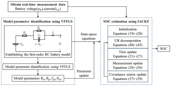
Figure 2.
The flowchart of SOC estimation framework.
4. Experiments
To successfully simulate the dynamics of LIBs under actual complex working conditions, a battery dataset, including the Beijing Dynamic Stress Test (BJDST) [52], the Federal Urban Driving Schedule (FUDS), and the Dynamic Stress Test (DST) at 0 °C, 25 °C, and 45 °C, was employed for evaluating the efficacy of the proposed SOC estimation method. The corresponding voltage and current profiles under the three driving cycles are plotted in Figure 3. The tested 18,650 lithium-ion battery has a nominal capacity of 2.0 Ah, and its lower discharging cut-off voltage is 2.5 V. The data sampling period is 1 s. Both the VFFLS and UR decomposition-based improved ACKF algorithms are programmed in MATLAB R2021a.
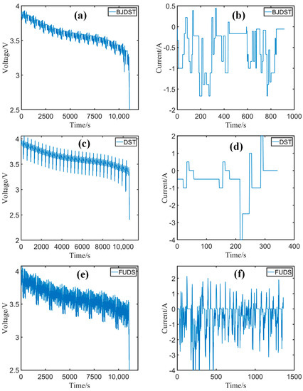
Figure 3.
Voltage and current profiles: voltage profiles of (a) BJDST, (c) DST, and (e) FUDS cycles; current profiles of (b) BJDST, (d) DST, and (f) FUDS cycles.
5. Validation Results and Discussion
5.1. Model Parameter Identification Results
In this section, the model parameter identification results at 25 °C will be presented and discussed. The parameters of first-order EECM are affected by many factors during charging and discharging, so in this paper, they are identified online by the improved VFFLS introduced in Section 2.2. The model parameter vector θ is initialized as [1 × 10⁻² 2 × 10⁻² 1 × 10⁻² 4], the multiple forgetting factors are [0.985 0.990 0.998 0.985], and the initial error covariance matrix P(0) is set as .
Parameter identification results of the first-order RC model are illustrated in Figure 4. It can be seen that the model parameters obviously vary at the end of discharging, i.e., at the range of high depth of discharging. To better quantify the accuracy of model parameter identification, herein, the measured battery terminal voltages are served as referenced values. Figure 5 presents the estimated terminal voltages from the battery model with the identified parameters in Figure 4, the reference terminal voltages, and the errors between them.
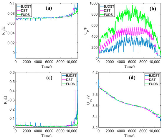
Figure 4.
The results of parameter identification at 25 °C: (a) Ro, (b)Cp, (c) Rp, and (d) Uoc.
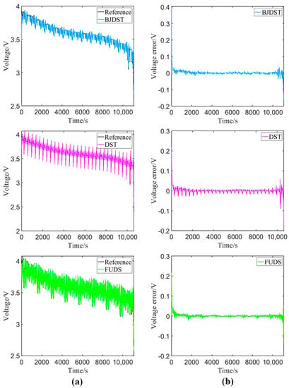
Figure 5.
Measured and estimated terminal voltage profiles: (a) voltage and (b) errors.
Table 1 lists the statistical results of the estimated terminal voltage errors, including the mean absolute error (MAE) and the root mean square error (RMSE). The MAE can avoid the cancellation between positive and negative errors, so it is usually employed to indicate the actual model error. The RMSE is applied to quantify the deviation between the estimated voltage and the referenced voltage. The MAE and RMSE can be formulated as follows:
where is the reference value, and represents the estimated value.

Table 1.
The errors between the estimated and reference terminal voltage.
It is clear from Table 1 that the MAE of the terminal voltage estimated by the first-order RC battery model with online parameter identification is lower than 5.1 mV, and the RMSE is within 11.2 mV. Hence, it can be concluded that the first-order RC battery model with the VFFLS-based online parameter identification has high accuracy and good adaptability to different driving cycles.
5.2. SOC Estimation Results
5.2.1. Results with Positive Definite Error Covariance Matrix
In this section, the SOC estimation at 25 °C is carried out with the configuration of the positive definite error covariance matrix for comparing the accuracy of the CKF family algorithms, including the CKF [53], ACKF [51], UR-CKF [46], and UR-ACKF. In actual working conditions, the initial SOC error occurs easily because of the capacity recovery of the battery, so it is important for the SOC estimators to have a high convergence speed for correcting an initial error quickly. Herein, to assess the correction capability of the algorithm to the initial SOC error, the initial SOC is set to 0.6, which is 0.2 lower than the actual value of 0.8. The error covariance matrix P, process noise matrix Q, and measurement noise matrix R are initially set in Equation (48).
The SOC estimation results with the aforementioned four algorithms are plotted in Figure 6. It is worth mentioning that the referenced SOC values are calculated using the ampere-hour integration method with accurate initial SOC and high-precision current measurements. To make a comparative study on the accuracy of the four CKF algorithms in more detail, the RMSE and MAE of the SOC estimation are calculated and the results are visualized in Figure 7.
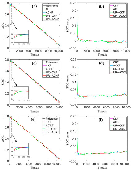
Figure 6.
The SOC estimation results of CKF family algorithms in a positive definite situation: (a,b) BJDST cycle; (c,d) DST cycle; (e,f) FUDS cycle.
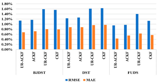
Figure 7.
The statistical results of SOC estimation using CKF family algorithms in a positive definite situation.
It is evident from Figure 6 and Figure 7 that all the CKF algorithms can operate properly under the condition of a positive definite error covariance matrix. Overall, the estimated SOC can precisely track the variation of the reference values. Under the same working conditions, the CKF and UR-CKF achieve very similar results, and the SOC estimation results of the ACKF and UR-AUKF are also consistent with each other. Taking the BJDST cycle as an example, the RMSEs of the UR-ACKF and ACKF are 1.14% and 1.17%, respectively, which are almost the same, and the MAEs are 0.68% and 0.72%, respectively. The reason is that, in theory, the factorizing results of a positive definite matrix with the Cholesky decomposition are equal to that with the UR decomposition. However, their actual factorizing results may be slightly different due to some reasons, such as random data truncation caused by the limitation of computer character length.
In addition, it can be seen from Figure 6 that the adaptive algorithms converge faster and the estimated SOC is more accurate compared with the non-adaptive algorithms, which can also be observed clearly from the statistical error results in Figure 7. For example, under the BJDST condition, the RMSE and MAE of UR-ACKF are 1.14% and 0.68%, respectively, while those of UR-CKF are 1.59% and 0.80%, respectively. This indicates that the CKF algorithms are unable to eliminate the impact of inaccurate initial parameters if the noise covariance matrices are not self-corrected, resulting in disordered changes in the SOC estimation error. Unlike the CKF, the ACKF algorithms present relatively orderly changes in estimation error, and they perform better in following the variations of the referenced SOC. Particularly, the proposed UR-ACKF algorithm achieves a RMSE of within 1.23% and a MAE of under 0.88%.
5.2.2. Results with Non-Positive Definite Error Covariance Matrix
In real-world applications, the situation of a non-positive definite error covariance matrix is likely to occur because of rounding and discretizing operations in hardware. Therefore, to simulate this situation, herein the error covariance matrix is initialized to be non-positive definite, as shown in Equation (49), and other conditions are kept unchanged. In this case, the Cholesky decomposition will fail to decompose the non-positive definite matrix, thus the CKF-family algorithms based on Cholesky decomposition no longer work. As a result, this section compares four different algorithms based on UR decomposition. To better reveal the advantages of the proposed SOC estimation method, in addition to the proposed VFFLS-ACKF, there is also the CKF based on the improved VFFLS parameter identification (VFFLS-CKF), the ACKF algorithms based on FFRLS parameter identification (FFRLS-ACKF) [25], and offline parameter identification (offline-ACKF). The forgetting factor λ is set as 0.98 for the FFRLS, and the offline parameter identification refers to the exponential fitting function method [54]. The comparative results of SOC estimation at 25 °C are shown in Figure 8, and the corresponding RMSE and MAE are visualized in Figure 9.
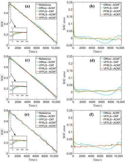
Figure 8.
The SOC estimation results and errors at 25 °C in a non-positive definite situation with CKF family algorithms of different battery tests. (a,b) BJDST cycle; (c,d) DST cycle; (e,f) FUDS cycle.
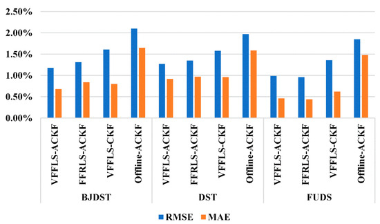
Figure 9.
The statistical results of SOC estimation at 25 °C using CKF family algorithm in a non-positive definite situation.
It is evident from Figure 8 and Figure 9 that the UR decomposition-based CKF algorithms can still operate normally even if the error covariance matrix is non-positive definite. In general, the estimated SOC values are highly consistent with the reference ones. For the two algorithms for online parameter identification, the VFFLS outperforms the FFRLS. For example, under the DST condition, the RMSE and MAE of VFFLS-ACKF are about 1.27% and 0.92%, respectively, while those of FFRLS-ACKF are about 1.35% and 0.97%, respectively.
It is also clear from Figure 8 that the SOC values estimated by the algorithm based on offline parameter identification deviate significantly from the references compared with those using the online parameter identification and are subjected to more fluctuation. Taking the BJDST cycle as an example, the RMSE and MAE of the VFFLS-ACKF are lower at 1.18% and 0.68%, respectively, while those of the offline-ACKF reach 2.10% and 1.65%, respectively, which are significantly larger than the former. This is because the internal parameters of LIBs vary continuously in practical working conditions. The online parameter identification can update the model parameters of LIBs correctly, so it can improve the accuracies of the battery model and SOC estimation.
5.2.3. Validation at Different Temperatures
The above experiments are conducted at 25 °C. In EV applications, the LIBs may operate under a wide range of temperatures, so it is important to evaluate the adaptability of the proposed algorithm to different temperatures. Therefore, in this section, the proposed method is further validated under BJDST conditions at 0 °C and 45 °C. The experiments also consider both cases of positive and non-positive definite error covariance matrices. The SOC estimation results are shown in Figure 10, while the RMSE and MAE are visualized in Figure 11.
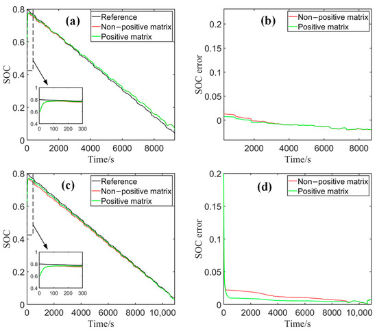
Figure 10.
The SOC estimation results and errors at different temperatures: (a,b) 0 °C; (c,d) 45 °C.
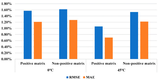
Figure 11.
The statistical results of SOC estimation at 0 °C and 45 °C.
From the results in Figure 10 and Figure 11, it can be concluded that under the BJDST condition, the SOC estimation errors at 0 °C are higher than those at 45 °C. The reason is that lithium-ion batteries may exhibit more complex nonlinear dynamic behavior at lower temperatures, resulting in a decrease in the accuracy of the first-order RC battery EECM. In addition, the RMSE remains within 1.62%, and the MAE remains within 1.27% at the two temperatures, indicating that the proposed method performs good adaptability to a wide temperature range.
6. Conclusions
This paper has proposed a SOC estimation method for lithium-ion batteries by incorporating a vector forgetting factor least square (VFFLS) algorithm and an improved adaptive cubature Kalman filter (ACKF). The VFFLS operation is implemented by substituting the single forgetting factor in the classical FFRLS method with multiple forgetting factors, enabling it to balance multiple parameters that change at different time scales. The Cholesky decomposition used in the standard CKF is substituted by the UR decomposition so that the filter can work no matter whether the error covariance matrix is positive or non-positive definite. In addition, an adaptive strategy for updating the noise covariances is introduced to the CKF. Statistical analysis of the RMSE and MAE of the predicted terminal voltage shows that the model parameters obtained by the VFFLS method can characterize the battery dynamics accurately. Experiments under DST, BJDST, and FUDS driving cycles at 25 °C demonstrate that the proposed method can work normally under both conditions of positive and non-positive definite error covariance matrices. Particularly, the RMSE is within 1.27%, and the MAE is within 0.92%. Compared with other algorithms, including the FFRLS-ACKF and offline-ACKF, the proposed method performs better in accuracy, stability, and convergence speed. In addition, validation under the BJDST cycle at 0 °C and 45 °C shows that the proposed method exhibits good adaptability to temperature.
The SOC estimation accuracy of LIBs is highly influenced by many factors. This work has provided a potential solution for the real-time battery management application of electric vehicles. However, there is still some room for improvement. In the future, we will further reveal the effect of battery aging on the efficacy of the proposed method. Moreover, the strategies for adaptively updating the multiple forgetting factors, which are helpful to the further efficacy improvement of the proposed method, are also worth investigating.
Author Contributions
Content organization and original draft preparation, Y.G.; conceptualization and supervision, J.T.; project administration and data curation, X.L.; validation and data curation, B.S.; review and delivery, Y.T. All authors have read and agreed to the published version of the manuscript.
Funding
This work was supported partly by the Science and Technology Plan Project of Shenzhen (No. JCYJ20220818100012026, No. 20220807222119001), the Natural Science Foundation of Guangdong Province (2021A1515010525), and the open research fund from Guangdong Laboratory of Artificial Intelligence and Digital Economy (SZ) (No. GML-KF-22-19).
Data Availability Statement
No new data were created. Data sharing is not applicable.
Conflicts of Interest
The authors declare no conflict of interest.
References
- Liu, Z.F.; Zhao, S.X.; Zhao, S.L.; You, G.D.; Hou, X.X.; Yu, J.L.; Li, L.L.; Chen, B. Improving the economic and environmental benefits of the energy system: A novel hybrid economic emission dispatch considering clean energy power uncertainty. Energy 2023, 285, 128668. [Google Scholar] [CrossRef]
- Ali, M.; Alkaabi, A.K.; Alameri, S.A.; Addad, Y. Overall efficiency analysis of an innovative load-following nuclear power plant-thermal energy storage coupled cycle. Int. J. Exergy 2021, 36, 98–122. [Google Scholar] [CrossRef]
- Xiong, R.; Kim, J.; Shen, W.X.; Lv, C.; Li, H.L.; Zhu, X.Y.; Zhao, W.Z.; Gao, B.Z.; Guo, H.Y.; Zhang, C.M.; et al. Key technologies for electric vehicles. Green Energy Intell. Transp. 2022, 1, 100041. [Google Scholar] [CrossRef]
- Shahjalal, M.; Roy, P.K.; Shams, T.; Fly, A.; Chowdhury, J.I.; Ahmed, M.R.; Liu, K. A review on second-life of Li-ion batteries: Prospects, challenges, and issues. Energy 2022, 241, 122881. [Google Scholar] [CrossRef]
- Liang, J.; Wu, T.; Wang, Z.; Yu, Y.; Hu, L.; Li, H.; Zhang, X.; Zhu, X.; Zhao, Y. Accelerating perovskite materials discovery and correlated energy applications through artificial intelligence. Energy Mater. 2022, 2, 200016. [Google Scholar] [CrossRef]
- Li, X.Y.; Huang, Z.J.; Hua, W.; Rao, L.; Tian, Y.; Tian, J. Mechanical vibration modeling and characterization of a plastic-cased lithium-ion battery. Green Energy Intell. Transp. 2022, 1, 100006. [Google Scholar] [CrossRef]
- Zhan, J.C.; Deng, Y.F.; Ren, J.Y.; Gao, Y.H.; Liu, Y.; Rao, S.; Li, W.F.; Gao, Z.H. Cell design for improving low-temperature performance of lithium-ion batteries for electric vehicles. Batteries 2023, 9, 373. [Google Scholar] [CrossRef]
- Yan, Y.; Zeng, T.; Liu, S.; Shu, C.Z.; Zeng, Y. Lithium metal stabilization for next-generation lithium-based batteries: From fundamental chemistry to advanced characterization and effective protection. Energy Mater. 2023, 3, 300002. [Google Scholar]
- Shrivastava, P.; Soon, T.K.; Idris, M.Y.I.B.; Mekhilef, S.; Adnan, S.B.R.S. Comprehensive co-estimation of lithium-ion battery state of charge, state of energy, state of power, maximum available capacity, and maximum available energy. J. Energy Storage 2022, 56, 106049. [Google Scholar] [CrossRef]
- Chen, C.; Xiong, R.; Yang, R.; Li, H. A novel data-driven method for mining battery open-circuit voltage characterization. Green Energy Intell. Transp. 2022, 1, 100001. [Google Scholar] [CrossRef]
- Guo, F.; Wu, X.W.; Liu, L.L.; Ye, J.L.; Wang, T.; Fu, L.J.; Wu, Y.P. Prediction of remaining useful life and state of health of lithium batteries based on time series feature and Savitzky-Golay filter combined with gated recurrent unit neural network. Energy 2023, 270, 126880. [Google Scholar] [CrossRef]
- Habib, A.K.M.A.; Hasan, M.K.; Issa, G.F.; Singh, D.; Islam, S.; Ghazal, T.M. Lithium-ion battery management system for electric vehicles: Constraints, challenges, and recommendations. Batteries 2023, 9, 152. [Google Scholar] [CrossRef]
- Chen, J.; Zhou, Z.; Zhou, Z.; Wang, X.; Liaw, B. Impact of battery cell imbalance on electric vehicle range. Green Energy Intell. Transp. 2022, 1, 100025. [Google Scholar] [CrossRef]
- Ng, K.S.; Moo, C.S.; Chen, Y.P.; Hsieh, Y.C. Enhanced coulomb counting method for estimating state-of-charge and state-of-health of lithium-ion batteries. Appl. Energy 2009, 86, 1506–1511. [Google Scholar] [CrossRef]
- Xing, Y.; He, W.; Pecht, M.; Tsui, K.L. State of charge estimation of lithium-ion batteries using the open-circuit voltage at various ambient temperatures. Appl. Energy 2014, 113, 106–115. [Google Scholar] [CrossRef]
- Mohammadi, F. Lithium-ion battery state-of-charge estimation based on an improved Coulomb-counting algorithm and uncertainty evaluation. J. Energy Storage 2022, 48, 104061. [Google Scholar] [CrossRef]
- Lee, S.; Kim, J.; Lee, J.; Cho, B.H. State-of-charge and capacity estimation of lithium-ion battery using a new open-circuit voltage versus state-of-charge. J. Power Sources 2008, 185, 1367–1373. [Google Scholar] [CrossRef]
- Tian, Y.; Lai, R.C.; Li, X.Y.; Tian, J.D. State-of-charge estimation for lithium-ion batteries based on attentional sequence-to-sequence architecture. J. Energy Storage 2023, 62, 106836. [Google Scholar] [CrossRef]
- Tian, J.P.; Xiong, R.; Shen, W.X.; Lu, J.H. State-of-charge estimation of LiFePO4 batteries in electric vehicles: A deep-learning enabled approach. Appl. Energy 2021, 291, 116812. [Google Scholar] [CrossRef]
- Anton, J.C.A.; Nieto, P.J.G.; Viejo, C.B.; Vilan, J.A.V. Support vector machines used to estimate the battery state of charge. IEEE Trans. Power Electron. 2013, 28, 5919–5926. [Google Scholar] [CrossRef]
- Malkhandi, S. Fuzzy logic-based learning system and estimation of state-of-charge of lead-acid battery. Eng. Appl. Artif. Intell. 2006, 19, 479–485. [Google Scholar] [CrossRef]
- Singh, P.; Vinjamuri, R.; Wang, X.; Reisner, D. Design and implementation of a fuzzy logic-based state-of-charge meter for Li-ion batteries used in portable defibrillators. J. Power Sources 2006, 162, 829–836. [Google Scholar] [CrossRef]
- How, D.N.T.; Hannan, M.A.; Lipu, M.S.H.; Ker, P.J. State of charge estimation for lithium-ion batteries using model-based and data-driven methods: A Review. IEEE Access 2019, 7, 136116–136136. [Google Scholar] [CrossRef]
- Zeng, Y.; Li, Y.; Yang, T. State of charge estimation for lithium-ion battery based on unscented Kalman filter and long short-term memory neural network. Batteries 2023, 9, 358. [Google Scholar] [CrossRef]
- Zhang, S.Z.; Guo, X.; Zhang, X.W. An improved adaptive unscented kalman filtering for state of charge online estimation of lithium-ion battery. J. Energy Storage 2020, 32, 101980. [Google Scholar] [CrossRef]
- Zhang, S.Z.; Zhang, C.; Jiang, S.Y.; Zhang, X.W. A comparative study of different adaptive extended/unscented Kalman filters for lithium-ion battery state-of-charge estimation. Energy 2022, 246, 123423. [Google Scholar] [CrossRef]
- Rahman, M.A.; Anwar, S.; Izadian, A. Electrochemical model parameter identification of a lithium-ion battery using particle swarm optimization method. J. Power Sources 2016, 307, 86–97. [Google Scholar] [CrossRef]
- Jokar, A.; Rajabloo, B.; Désilets, M.; Lacroix, M. Review of simplified Pseudo-two-Dimensional models of lithium-ion batteries. J. Power Sources 2016, 327, 44–55. [Google Scholar] [CrossRef]
- He, H.W.; Xiong, R.; Fan, J.X. Evaluation of lithium-ion battery equivalent circuit models for state of charge estimation by an experimental approach. Energies 2011, 4, 582–598. [Google Scholar] [CrossRef]
- Nejad, S.; Gladwin, D.T.; Stone, D.A. A systematic review of lumped-parameter equivalent circuit models for real-time estimation of lithium-ion battery states. J. Power Sources 2016, 316, 183–196. [Google Scholar] [CrossRef]
- Tian, Y.; Huang, Z.J.; Long, T.; Tian, J.D.; Li, X.Y. Performance analysis and modeling of three energy storage devices for electric vehicle applications over a wide temperature range. Electrochim. Acta 2020, 331, 135317. [Google Scholar] [CrossRef]
- Ling, L.; Sun, D.M.; Yu, X.L.; Huang, R. State of charge estimation of Lithium-ion batteries based on the probabilistic fusion of two kinds of cubature Kalman filters. J. Energy Storage 2021, 43, 103070. [Google Scholar] [CrossRef]
- Zhang, C.; Allafi, W.; Dinh, Q.; Ascencio, P.; Marco, J. Online estimation of battery equivalent circuit model parameters and state of charge using decoupled least squares technique. Energy 2018, 142, 678–688. [Google Scholar] [CrossRef]
- Ouyang, T.C.; Xu, P.H.; Chen, J.X.; Lu, J.; Chen, N. Improved parameters identification and state of charge estimation for lithium-ion battery with real-time optimal forgetting factor. Electrochim. Acta 2020, 353, 136576. [Google Scholar] [CrossRef]
- Ge, C.A.; Zheng, Y.P.; Yu, Y. State of charge estimation of lithium-ion battery based on improved forgetting factor recursive least squares-extended Kalman filter joint algorithm. J. Energy Storage 2022, 55, 105474. [Google Scholar] [CrossRef]
- Duong, V.H.; Bastawrous, H.A.; Lim, K.; See, K.W.; Zhang, P.; Dou, S.X. Online state of charge and model parameters estimation of the LiFePO4 battery in electric vehicles using multiple adaptive forgetting factors recursive least-squares. J. Power Sources 2015, 296, 215–224. [Google Scholar] [CrossRef]
- Song, Q.; Mi, Y.X.; Lai, W.X. A novel variable forgetting factor recursive least square algorithm to improve the anti-interference ability of battery model parameters identification. IEEE Access 2019, 7, 61548–61557. [Google Scholar] [CrossRef]
- Tang, J.; Liu, S.Q.; Liu, J.W.; Liu, Q.S.; Zhao, Y.; Lian, Z.X. Parameter identification in urban rail train energy storage elements using a vector multi-forgetting factor least square method. Eng. J. Wuhan Univ. 2020, 53, 527–533. (In Chinese) [Google Scholar]
- Dai, H.F.; Xu, T.J.; Zhu, L.T.; Wei, X.Z.; Sun, Z.C. Adaptive model parameter identification for large capacity Li-ion batteries on separated time scales. Appl. Energy 2016, 184, 119–131. [Google Scholar] [CrossRef]
- Hossain, M.; Haque, M.E.; Arif, M.T. Kalman filtering techniques for the online model parameters and state of charge estimation of the Li-ion batteries: A comparative analysis. J. Energy Storage 2022, 51, 104174. [Google Scholar] [CrossRef]
- Khan, Z.A.; Shrivastava, P.; Amrr, S.M.; Mekhilef, S.; Algethami, A.A.; Seyedmahmoudian, M.; Stojcevski, A. A comparative study on different online state of charge estimation algorithms for lithium-ion batteries. Sustainability 2022, 14, 7412. [Google Scholar] [CrossRef]
- Arasaratnam, I.; Haykin, S. Cubature Kalman filters. IEEE Trans. Autom. Control 2009, 54, 1254–1269. [Google Scholar] [CrossRef]
- Liu, Z.; Dang, X.J.; Jing, B.Q.; Ji, J.B. A novel model-based state of charge estimation for lithium-ion battery using adaptive robust iterative cubature Kalman filter. Electr. Pow. Syst. Res. 2019, 177, 105951. [Google Scholar] [CrossRef]
- Wang, Y.C.; Meng, D.W.; Chang, Y.J.; Zhou, Y.Q.; Li, R.; Zhang, X.Y. Research on online parameter identification and SOC estimation methods of lithium-ion battery model based on a robustness analysis. Int. J. Energy Res. 2021, 45, 21234–21253. [Google Scholar] [CrossRef]
- Li, K.Q.; Zhou, F.; Chen, X.; Yang, W.; Shen, J.J.; Song, Z.B. State-of-charge estimation combination algorithm for lithium-ion batteries with Frobenius-norm-based QR decomposition modified adaptive cubature Kalman filter and H-infinity filter based on electro-thermal model. Energy 2023, 263, 125763. [Google Scholar] [CrossRef]
- Tian, Y.; Huang, Z.J.; Tian, J.D.; Li, X.Y. State of charge estimation of lithium-ion batteries based on cubature Kalman filters with different matrix decomposition strategies. Energy 2022, 238, 121917. [Google Scholar] [CrossRef]
- Wang, C.; Xu, M.Y.; Zhang, Q.J.; Feng, J.H.; Jiang, R.Z.; Wei, Y.; Liu, Y.C. Parameters identification of Thevenin model for lithium-ion batteries using self-adaptive particle swarm optimization differential evolution algorithm to estimate state of charge. J. Energy Storage 2021, 44, 103244. [Google Scholar] [CrossRef]
- Paleologu, C.; Benesty, J.; Ciochina, S. A robust variable forgetting factor recursive least-squares algorithm for system identification. IEEE Signal Proc. Lett. 2008, 15, 597–600. [Google Scholar] [CrossRef]
- Stefanopoulou, A. Recursive least squares with forgetting for online estimation of vehicle mass and road grade: Theory and experiments. Vehicle Syst. Dyn. 2005, 43, 31–55. [Google Scholar]
- Tian, Y.; Lai, R.C.; Li, X.Y.; Xiang, L.J.; Tian, J.D. A combined method for state-of-charge estimation for lithium-ion batteries using a long short-term memory network and an adaptive cubature Kalman filter. Appl. Energy 2020, 265, 114789. [Google Scholar] [CrossRef]
- Zeng, Z.B.; Tian, J.D.; Li, D.; Tian, Y. An online state of charge estimation algorithm for lithium-ion batteries using an improved adaptive cubature kalman filter. Energies 2018, 11, 59. [Google Scholar] [CrossRef]
- Yang, K.; Tang, Y.G.; Zhang, S.J.; Zhang, Z. A deep learning approach to state of charge estimation of lithium-ion batteries based on dual-stage attention mechanism. Energy 2022, 244, 123233. [Google Scholar] [CrossRef]
- Peng, J.K.; Luo, J.Y.; He, H.W.; Lu, B. An improved state of charge estimation method based on cubature Kalman filter for lithium-ion batteries. Appl. Energy 2019, 253, 113520. [Google Scholar] [CrossRef]
- Lu, L.G.; Han, X.B.; Li, J.Q.; Hua, J.F.; Ouyang, M.G. A review on the key issues for lithium-ion battery management in electric vehicles. J. Power Sources 2013, 226, 272–288. [Google Scholar] [CrossRef]
Disclaimer/Publisher’s Note: The statements, opinions and data contained in all publications are solely those of the individual author(s) and contributor(s) and not of MDPI and/or the editor(s). MDPI and/or the editor(s) disclaim responsibility for any injury to people or property resulting from any ideas, methods, instructions or products referred to in the content. |
© 2023 by the authors. Licensee MDPI, Basel, Switzerland. This article is an open access article distributed under the terms and conditions of the Creative Commons Attribution (CC BY) license (https://creativecommons.org/licenses/by/4.0/).