Abstract
A typical method for measuring the radial thermal conductivity of cylindrical objects is the pipe method. This method introduces a heating wire in combination with standard thermocouples and optical Fiber Bragg grating temperature sensors into the core of a cell. This experimental method can lead to high uncertainties due to the slightly varying setup for each measurement and the non-homogenous structure of the cell. Due to the lack of equipment on the market, researchers have to resort to such experimental methods. To verify the measurement uncertainties and to show the possible range of results, an additional method is introduced. In this second method the cell is disassembled, and the thermal conductivity of each cell component is calculated based on measurements with the laser flash method and differential scanning calorimetry. Those results are used to numerically calculate thermal conductivity and to parameterize a finite element model. With this model, the uncertainties and problems inherent in the pipe method for cylindrical cells were shown. The surprising result was that uncertainties of up to 25% arise, just from incorrect assumption about the sensor position. Furthermore, the change in radial thermal conductivity at different states of charge (SOC) was measured with fully functional cells using the pipe method.
1. Introduction
Cylindrical Lithium-ion secondary battery (LIB) cells can be found in many devices such as consumer products as well as electric cars due to their energy density of up to 270 Wh/kg, their high cycle stability, intrinsic safety, high availability and relatively low cost [1,2]. In order to ensure safe operation and to maximize service life, the thermal boundaries of LIB cells must be respected all the time. For a proper module and system design, it is crucial to know in advance the thermal properties like heat generation during operation as well as the thermal conductivity and heat capacity of the cell [3,4,5]. Current battery management systems (BMS) measure the surface temperature of cells to check whether their temperature limits have been exceeded. In most cases, the cell temperature is only measured at pre-selected points in a module. However, this surface temperature can differ greatly from the internal (core) temperature of the cell. Depending on the C-rate, a temperature difference of up to 15 C can occur [6]. In extreme situations such as a thermal runaway, the difference between internal and external temperature can be even higher. In this case temperature sensors mounted on the surface would show an increased temperature only after a certain time delay. With precise estimation models or with additional internal temperature sensors, such an event could be detected earlier. Due to the fast thermal buildup of such an event, a fast detection is necessary to shut off all processes like charging or discharging which might aggravate the actual state. The effective thermal conductivity in radial and axial direction shown in Table 1 is necessary to estimate the thermal propagation during, for example, a thermal runaway of a single cylindrical cell in a battery pack.
In addition, there is also a trend towards bigger cells, such as the 4680 form factor. This form factor means a 46 mm diameter and a 80 mm height of the cylindrical cell, which leads to an increase of the volume by a factor of eight in comparison to an 18650 cell geometry. Especially in automotive applications, attempts are made to use the space within battery packs more effectively. However, due to larger cells, there can also be greater inhomogeneities in cell temperature. As this work will show, even the inhomogeneous shape of the bulk material can cause fluctuations in the thermal conductivity. Precise knowledge of the thermal conductivity plays an important role for thermal models within a BMS and for the thermal design of the battery pack. Figure 1 shows possible directions of heat flow in cylindrical cells or pouch cells. When measuring the thermal conductivity of cylindrical cells, the effective radial and axial thermal conductivity is measured. In the case of pouch cells, the effective in-plane and out-of-plane thermal conductivity is typically measured.
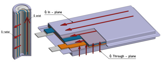
Figure 1.
Different heat flow directions in cylindrical cells and pouch cells.
The heat rate and heat capacity of cylindrical cells can already be measured well with commercial, reliable equipment such as calorimeters [7]. However, to the knowledge of the authors, no suitable device is available for the measurement of the effective radial thermal conductivity of cylindrical cells. Therefore, only experimental methods like the pipe method explained in Section 1.1 can be used. The literature research, which follows in the next paragraph, shows that most researchers chose a single method without documented reference measurements.
In [8], they used a flexible Kapton heater on the top or on the curved surface of the cell to heat in radial or axial direction. T-Type thermocouples are attached in various location along the cell outer wall or on the top of the cell to measure the axial or radial thermal conductivity. The thermal conductivity is then calculated by comparison with an analytical model. Yang et al. [9] measured the thermal conductivity of the separator with the hot plate method, which is part of the steady state methods explained in Section 1.1. To reduce the influence of the thermal resistance, multiple layers of separators were stacked together. In [10] the effective radial thermal conductivity is measured using the pipe method with a nichrome wire in the center of the cell and type K thermocouples on the inside and the outside of the cell.
Table 1 shows different values which can be found in literature for the thermal conductivity of cylindrical cells. Furthermore it shows the in-plane and out-of-plane conductivity of single anode and cathode layers, as well as the thermal conductivity of the separator.

Table 1.
Values found in literature for the thermal conductivity of cylindrical cells and their individual layers.
Table 1.
Values found in literature for the thermal conductivity of cylindrical cells and their individual layers.
| Material/Layer | Cross-Plane | In-Plane | Geometry | Capacity | Refs. | ||
|---|---|---|---|---|---|---|---|
| [Wm−1·K−1] | [Wm−1·K−1] | [Wm−1·K−1] | [Wm−1·K−1] | [Ah] | |||
| NMC, LCO, NCA | 0.15–2.59 | 1.78–32 | 18650 | 2.14–3.5 | [8,10,11,12,13] | ||
| 3 | 21,700 | [11] | |||||
| 0.2 | 30.4 | 26,650 | [8,10] | ||||
| Single Layer | |||||||
| LiCoO2 (LCO) (Cathode) | 1.58–3.5 | 21.6–28 | [5,9,14,15] | ||||
| Graphite (Anode) | 0.89–1.2 | 8.72–139 | [9,14,15,16] | ||||
| Separator | 0.1–1 | [9,14,16,17] |
As shown in Table 1, the effective radial thermal conductivity found in literature varies between 0.15 and 2.59 Wm−1·K−1. Using the data found in the references [8,10,11,12,13], for the radial thermal conductivity for 18650 cells, a standard deviation of 1.61 Wm−1·K−1 can be calculated, which can be considered very high, especially compared to the actual measured values. Therefore, this paper’s objective is to analyze the experimental process and to identify reasons why these deviations in the radial thermal conductivity occur when the pipe method is used.
To pursue this goal, two different methods are used, the first one being the pipe method and the second one being a combination of the laser flash method (LFA) and differential scanning calorimetry (DSC). To eliminate all unknowns in the measurement setup, reference measurements were conducted with materials, for which the exact value of the thermal conductivity can be found in literature (see Section 2.3). The first measurement results with the reference samples showed high deviations compared to the thermal conductivities that are common in the literature for these materials. To counteract these high uncertainties, several improvements of the measurement setup were made. This includes, among other things, the usage of optical Fiber Bragg grating (FBG) sensors, which offer a higher precision in comparison to standard type K thermocouples. Furthermore, a thermal paste with a high thermal conductivity (5 Wm−1·K−1) was used to reduce the influence of the contact resistance. Even with these improvements, the deviation of the radial thermal conductivity could not be adequately reduced. Therefore, a second independent method, which was intended to further limit the possible range of results, was introduced. This second method calculates the effective thermal conductivity from the results of the LFA and DSC measurements that are described in Section 1.2. However, this second method is not intended to serve as a benchmark, since the cell must be completely disassembled and therefore influences like the missing electrolyte cannot be considered. Using this second method, the thermal conductivity values of each of the materials of a LIB were established, which made it possible to create a simplified FEM-model that depicts the measurement setup of the pipe-method for a cylindrical cell. With the help of this thermal simulation, the authors were able to show that not only the slightest changes in the measurement setup can lead to major variations. Furthermore, a minor deviation in the structure of the cell can lead to a major variation in the measured thermal conductivity. For the first time, uncertainties in the pipe method used for LIB-based thermal conductivity measurements were analyzed in detail. In addition to this discovery, the authors also investigated the influence of the separator on the thermal conductivity and analyzed the state-of-charge (SOC) dependency of the thermal conductivity on functional cells. Figure 2 shows the flowchart of the methods used, including the process to measure or calculate the radial thermal conductivity.
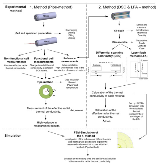
Figure 2.
Flowchart of the methods used, including a description of the performed steps.
1.1. Steady-State Methods
A typical method for determining the thermal conductivity is the heat flow meter (HFM) method, which is similar to the single-specimen guarded hot plate method. This method belongs to the steady-state methods whereby the thermal conductivity [Wm−1·K−1] can be calculated after the system reaches a steady state, which is the case when the heat flux through the specimen is constant. This method uses two calibrated heat flux sensors to measure the heat flux density [W/m2]. With known sensor area, the heat flux [W] through the specimen can be calculated. Therefore, the specimen is put between a heated and a cooled plate. With a defined temperature gradient and the measured heat flux, the thermal conductivity of the specimen can be calculated according to Equation (1).
It should be noted that this method in comparison to other methods needs a relatively thick specimen if materials with high thermal conductivity should be measured. When increasing the thickness of the specimen, the thermal resistance of the sample increases and the influence of the thermal contact resistance on the measurement result decreases [18,19]. This method works well for pouch cells where the heating and cooling plate can be fully attached on the surface area of the flat cell. However, for 18650 cells this measurement method is not suitable, as, due to the cylindrical shape, the heat flux will not distribute evenly.
The pipe method, which is also one of the steady-state methods, can be used to directly measure the radial thermal conductivity of a cylindrical cell. A heating rod or heating wire is inserted axisymmetrically into the sample, which transfers the heat evenly to the surrounding material. This creates a uniform heat flux from the inside to the outside of the cylinder. The heat flux can be determined via the power losses of the heating wire or with the help of a heat flux sensor. Temperature sensors mounted on the inner and outer surface measure the temperature difference. Axial heating losses should be avoided with insulation material or with the help of active heating on the front surface of the cylinder. By using the pipe method, the radial thermal conductivity for a cylindrical wall can be calculated, depending on the number of considered layers using Equation (2) or (3).
When using the pipe method, an exact knowledge of the heating wire and temperature sensor position is important. Due to the small space (∼3.8 mm) in the center of 18650 cells, it is difficult to place the temperature sensor on the inner surface of the cell winding. To minimize the thermal resistance between the sensor and the cell surface, it is important to use a thermal paste with high conductivity, which is also difficult to position within the cell. Using an ideal model assuming perfect thermal contact between each layer shows that the results of direct measurements can be strongly influenced by unknown or wrong assumptions about the position of the temperature sensor and heating wire. Missing thermal paste or a non-ideal circular shape of the cell winding can also influence the direct measurement method.
1.2. Transient Methods
Transient methods are another way of measuring the thermal conductivity. These include, for example, the laser flash method (LFA) together with the differential scanning calorimetry (DSC) technology, as well as the hot wire method. These methods analyze the transient response of the temperature versus time. During this process, the thermal diffusivity can be determined with the sample thickness and the measured half time as shown in Equation (4) [20].
An advantage of the LFA method is that it eliminates thermal contact resistance problems. To determine the heat capacity of the different battery layers, a DSC was used. Part of the DSC are two pans. In the first pan, the specimen was placed, and in the second one, a reference material. The temperatures of the reference material and the specimen are measured and compared after heating up both pans equally. If the sample material has the same thermal properties as the reference material, the heat flow between the materials and the furnace is also identical. If the heat flow changes due to different material parameters, a temperature difference is measured. With the measured temperature difference and a previously determined calibration coefficient, the heat flow can be calculated. Integration of the heat flow over time results in the total amount of heat Q. The specific heat capacity can finally be calculated with the following equation [21]:
The thermal conductivity can now be calculated using the thermal diffusivity and the heat capacity as well as the density:
The thermal conductivity can thus be calculated using the measurement results from the LFA and the DSC measurements. This is one approach to separately measure the thermal conductivity of each layer of the battery.
2. Experimental Method
To evaluate the uncertainties and to limit the possible range of results, two approaches were chosen to determine the radial thermal conductivity. The first approach utilizes the pipe method and directly measures the conductivity of the bulk material and the case of the cell. The second approach is to separately determine the material parameters of each layer and calculate the thermal conductivity of the cell afterwards analytically or by simulation. For the pipe method approach, two different types of temperature sensors were used. In the first measurement setup, a standard Type K-based thermocouple is used to determine the temperature difference. The second setup measures the temperature with optical Fiber Bragg grating (FBG) sensors. The FBG-based setup offers some advantages compared to the thermocouple-based setup. The FBG sensors offer a higher accuracy and within one fiber, multiple sensors can be measured. This can improve the measurement accuracy when measuring materials or objects with higher thermal conductivities.
2.1. Thermocouple Based Setup
Figure 3 shows the measurement setup using type K thermocouples. For the inner temperature measurement, thermocouples with a diameter of 0.5 mm are used. The tip is made of stainless steel, which is long-term stable to the chemical environment in the cell. The wire and the junction are electrically insulated from the casing, so the potential in the cell does not influence the measurement. For the measurements inside the cylinder, relatively thin temperature sensors should be used to leave enough space for several windings of heating wire. The used thermocouples meet the tolerance class 1 ± 1.5 C) according to IEC 584.
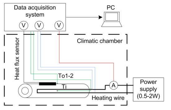
Figure 3.
Thermocouple-based measurement setup.
The temperature sensors were compared with a calibrated PT100 which has a measurement uncertainty of . The maximum measured temperature deviation was 0.53 C. The used enameled copper wire had a diameter of 0.4 mm. Multiple windings of copper wire were used to heat up the specimen. The varnish was removed at the end of the cylinder and the voltage drop, and thus the power loss was measured via the current. The heat flux sensor type FHF03 from Hukseflux had a sensitivity of V/(W/m and a calibration uncertainty of V/(W/m according to the datasheet. The heat flux sensor had a sensing area of m2. The heat flow can be calculated according to Equation (7)–(9).
The heat flux sensor was used to compare the measured heat flow with the steady state power dissipation. The final assembled cylinder was then placed in a box to minimize the influence of drafts. The measurement data was recorded periodically using a data acquisition system. The thermal conductivity measurements were carried out within a climatic chamber at 20 C.
2.2. FBG Sensor-Based Setup
Figure 4 shows the measurement setup using FBG sensors. Two fibers with two measurement points; hence, two FBGs are used. A glass capillary protects the FBGs and serves as strain compensation. Due to the capillary, the diameter of the sensors is 0.25 mm. Even with a capillary protecting the fiber, the sensor is thinner than the thermocouples, which allowed the integration of an additional heating wire. One sensor is attached to the housing of the 18650 cell and one is inside the cell together with the copper wire.
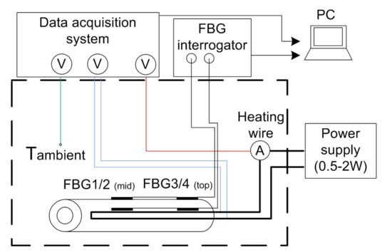
Figure 4.
FBG-based measurement setup.
Previously the FBG sensors were calibrated in a climatic chamber type WKL 100 from Weiss in an aluminum block. A HYPERION si155 interrogation unit from Luna Inc. (Roanoke, VA, USA) was used for data acquisition. A precision thermometer type T4200 from Dostmann electronic monitored the temperature of the aluminum block. This reference thermometer has an accuracy of 15 mK. The temperature range was between 25 C and 80 C. Each temperature was kept for 45 min to ensure equilibrium. In Figure 5, the calibration curve for one FBG is shown. In Table 2, the sensitivities for all the used FBGs are listed.
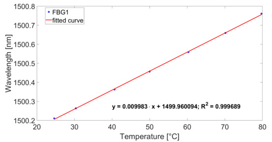
Figure 5.
Calibration curve for FBG1 from Sensor 1.
Table 2.
Sensitivity of each FBG.
2.3. Reference Material Measurements
Before the measurements on the 18650 LIB started, two materials with known thermal conductivity were measured in order to validate the measurement setup. The reference materials were chosen such that their radial thermal conductivities are within the expected ranges for the cell. If the measurement technique works for both reference values, it can be assumed that it also works for values in between. One specimen of acrylic glass ( Wm−1·K−1), which represents the lower range of thermal conductivity for this setup, and one specimen of fused quartz ( Wm−1·K−1), which represents the upper bound of this measurement setup, were selected. The dimensions of the reference materials were chosen to be comparable to those of the cylindrical cell, to ensure similar conditions as for the measurements conducted later. According to Equation (2) the expected for Polymethylmethacrylate (PMMA) is 32 C and for fused quartz it is 10 C. Therefore, the influence in temperature measurement uncertainty increases the greater the thermal conductivity of the reference material is.
To determine whether the thermal conductivity value can be measured more precisely by using the more expensive FBGs, these sensors were additionally placed on the fused quartz, where the possible measurement variance caused by the lower together with the accuracy of the sensors is higher. The sensors and the heating wire were placed inside and outside the specimen as shown in Figure 3 and Figure 4. Figure 6 shows the step response of the different specimen.
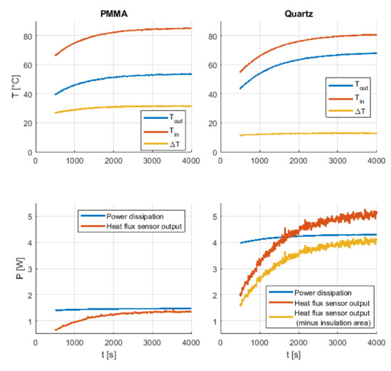
Figure 6.
Reference material measurements carried out with the thermocouple-based measurement setup: measured temperatures and dissipation power from the PMMA specimen (left side) and from the Quartz-specimen (right side).
For the PMMA specimen, which can be seen on the left side in Figure 6, a difference in the measured power dissipation and the heat flux sensor output occurs in the steady state area. This 0.26 W difference could be explained by the cylindrical form of the specimen, which caused a poor surface contact with parts of the heat flux sensor. To avoid this problem, zip ties were used to mount the heat flux sensor in an axial direction, due to its low radial bending radius of 25 mm. Additionally, thermal paste was used between the sensor and the cylinder to reduce the thermal resistance. Another important thing that can be seen in Figure 6 is that due to the rising temperature of the heating wire, which leads to an increase in its electrical resistance, the dissipation power also increases over time. To obtain a constant power over the duration of the measurement, a control loop would be needed. However, the heating wire reaches its maximum temperature after a certain time, which leads to a constant heat flow. It can take more than one hour until the steady state is reached, which is a big disadvantage compared to transient methods where the result is available after a short measurement time. With the measurement results (Figure 6) it is now possible to calculate together with Equation (3) the thermal conductivity, which is Wm−1·K−1 for the PMMA cylinder. For the fused quartz cylinder, a 0.75 W higher heat flow compared to the steady-state power dissipation was measured. For these measurements the insulation material, which was put on the poles to mitigate axial heat flow, partially covered some surface area of interest, leading to a reduced surface area for heat dissipation. If the fused quartz cylinder area is reduced by the area of the insulation material, the calculated heat flow is 0.25 W smaller than the measured power dissipation. Using the heat flow based on the reduced cylinder area leads to Wm−1·K−1 for the fused quartz cylinder.
Table 3 shows the dimensions used and the measured data from the steady-state condition together with the measured and known thermal radial conductivities. The ranges for the measured thermal conductivity is due to the temperature measurements at two different positions on the specimen.
Table 3.
Measurement results of the pipe method for the reference materials.
To better point out the difference between the measured values and the values from literature, the relative measurement uncertainty was calculated by computing the difference between them. These differences are then related to the literature value and multiplied by 100 to get the percentage.
A measurement uncertainty of 4.9% for the thermocouple-based setup and an uncertainty of 12.7% for the FBG-based setup was achieved for the quartz specimen. For the PMMA specimen measurement an uncertainty of 3.7% was achieved.
According to these results, the calculated radial thermal conductivities are surprisingly less precise with the FBGs than with the thermocouples. From this, it can be concluded that the accuracy of the temperature sensor is not the main influencing factor in the measurement uncertainty. Thus, in this section the goal of validating the test setup for the possible values in which the thermal conductivity for 18650-cells might lie, was achieved. A closer look at the problems of the positioning of the sensors and possible other factors for the cylindrical cell will be undertaken in the following chapters.
2.4. 18650 Cell Measurements
The section below shows the methods used for the 18650 cell measurements.
2.4.1. Pipe Method Inactive Cell Measurements
Seven Samsung INR18650-25R cells with lithium nickel cobalt aluminum oxide (NCA) as cathode material and graphite as anode material were prepared for the measurements. Five of them (C1–C5) were discharged to 0.1 V with a C/2 rate, and the potential was held until the current reached C/50. This allowed for safely drilling a hole in the terminal of the cell, filling it with thermal paste and inserting a heating wire and temperature sensor. Finally, the drilled hole was closed with an epoxy glue. The weight of the cells was measured before and after to see if enough thermal paste was inserted in the free space in the middle of the cell. One cell was only discharged to the minimum recommended cell voltage of 2.5 V to keep the cell functional after preparation. This cell was not filled with thermal paste. Another cell was disassembled to estimate the layer thickness and the structure of the cell. Furthermore, samples of the anode and cathode material as well as samples from the housing were obtained for analysis with the LFA and a DSC. Figure 7 shows the prepared cell as well as the heating wire with the additional FBG sensor before plugging it into the cell.
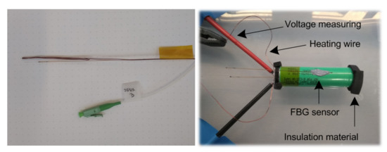
Figure 7.
Heating wire together with the FBG sensor (left) and the prepared cell (right).
Table 4 shows the dimensions of the cell, the temperature difference between the inside and outside of the cell, the heat flow and the effective thermal conductivities obtained by the pipe method. The effective thermal conductivity was calculated using Equation (3). The ranges for the effective thermal conductivity are due to multiple sensor measurements.
Table 4.
Measurement results of the pipe method for the 18650 cells.
Using Equation (3) leads to several assumptions. The first assumption is that the thermal paste is equally distributed in the inner hole of the cell. The second assumption is that the heating wire is located exactly in the center of the cell and radiates the heat evenly. In addition, it is assumed that the temperature drop between the heating wire and the surface of the internal bulk material is negligible, since the thermal paste has a significantly higher thermal conductivity than the cell. The effective radial thermal conductivity of the measured cells is between Wm−1·K−1 and Wm−1·K−1. Due to safety reasons the maximum inner temperature of the cell was limited to 55 C, which also limits the maximum power dissipation and therefore the maximum temperature difference between the inner and outer surface of the cell. The temperature difference achieved in the measurements varies between 6.8 C and 12 C depending on the power dissipation. Except for cell number 4, two temperature sensors were mounted on the outer surface of each cell. For the thermocouple-based setup each temperature sensor is mounted with thermal adhesive on the middle of the cell on different sides. Between these outer temperature sensors, a maximum difference of 1 C occurred. This can happen due to the tolerance of each temperature sensor, but also because of uneven distributed heat. Due to the high fluctuations in the individual measurement results, the influence in heating wire and sensor position will be analyzed more accurately in the simulation chapter.
2.4.2. Measurements at Different State of Charge (SOC) Levels Using the Pipe Method
The prepared still-functional cell is used to measure the effective thermal conductivity at different SOC levels. To calculate the effective radial thermal conductivity at different SOC levels, the cell was charged to 50% and 100% SOC by applying a constant current (CC) phase with 0.5C, followed by a constant voltage (CV) phase with 3.7 V and 4.2 V, respectively. The termination criterion for the CV phase was reached when the current was less than 0.05C. After finishing the charging process, a relaxation phase of 30 min was introduced. Subsequently, the thermal conductivity measurement was started. After heating up the cell and performing the measurements, the heating was stopped and the cell was allowed to cool down and to reach equilibrium state again. This procedure was repeated at each SOC level. Figure 8 shows that the thermal conductivity rises slightly at 100% SOC.
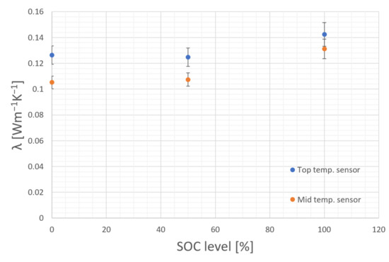
Figure 8.
SOC dependency of the effective thermal conductivity.
The used cell is the only one without thermal paste between the heating wire and the inner bulk material of the cell to maintain operation. Therefore, the thermal conductivity between the heating wire and the inner surface of the cell is low resulting in a high temperature difference between the outer and inner sensor. Due to the high temperature difference, caused by the high thermal resistance between the heating wire and the bulk material, the measured values do not represent the effective thermal conductivity of the cell. The estimated values should not be used for further simulations or calculations. For this measurement only the difference in effective thermal conductivity between the different SOC levels is relevant. The active material used for LIB is subjected to permanent changes both during a cycle as well as over its lifetime. Insertion and subtraction of Lithium-ions (Li) leads the materials to expand and contract upon charge or discharge [22]. Graphite, which is commonly used as anode-active material for commercial cylindrical cells [1], shows an expansion of around 10%, while cathode-active materials usually exhibit smaller changes [22]. Due to the layered structure of LIB those thickness changes are superimposed. As the anode exhibits higher changes in volume over the SOC it is the dominant part during cycling. The degree of lithiation for the anode is highest at SOC 100%, meaning a fully charged cell. This is where prismatic LIB cells usually show their greatest thickness [23,24] or cylindrical cells show their greatest diameter [25]. In cylindrical cells this also leads to surface strain [26] caused by the mechanical force arising from the bulk materials. As these forces are significant enough to deform the metal can of a cylindrical cell, the authors of this work assume that also the heat conductivity of the cell might change during cycling as both the density of the bulk as well as the contact between each surface changes. The higher the pressure in the bulk material, the higher the radial thermal conductivity.
2.4.3. LFA and DSC Based Cell Measurements
Besides the pipe method, another approach to measure the effective thermal conductivity of a cylindrical cell is to analyze each layer separately with the laser flash method and a differential scanning calorimeter. By knowing the thermal conductivity of each layer, the thermal resistance can be calculated according to Equation (10) [27]:
To obtain the size and the number of each layer in radial direction a computerized tomography (CT) scan of the same cell type was taken. To simplify the calculation, the total thickness of each layer (anode, cathode and separator layer) is summed up. Figure 9 shows the CT scans of the cell. These scans were taken with an X-ray Inspection system of type XT V 160 from Nikon. With these pictures it was possible to count the number of each layer in radial direction and to estimate the diameter of the inner hole. Furthermore, it is possible to measure the thickness of each layer.
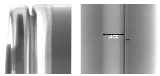
Figure 9.
CT scan of the cell showing the different layers and the diameter of the inner hole (Left: A horizontal scan of an 18650 cell. Right: Vertical scan showing the diameter of the inner hole).
Table 5 shows the measured thickness of each cell layer including the case. Summing up all layer thicknesses including the radius of the inner hole leads to a cell radius of 9042 µm.
Table 5.
Thickness and number of the different cell layer.
After measuring the thickness of each layer, the anode and cathode layer as well as the cell case specimen were analyzed with the LFA. For the LFA-based measurements the HyperFlash system type LFA 467 from Netzsch was used. Thereby the thermal diffusivity of each specimen was measured. With the differential scanning calorimeter, the heat capacity can be measured. For this purpose, the heat-flux DSC system type 204 F1 Phoenix from Netzsch was used. Using the density of the specimen, the thermal conductivity according to Equation (6) can be calculated. Table 6 shows the results of the LFA and the DSC measurements.
Table 6.
LFA and DSC measurement results.
Because of the transparency and the low thickness of the separator it could not be measured as the laser did not heat the material but penetrated it. Common polymer-based separators have a thermal conductivity as low as 0.1–0.5 Wm−1·K−1 [9,14,16,17]. Therefore, they have a great impact on heat transfer in the cell [9]. By varying the value of the thermal conductivity of the separator within the previously mentioned range and calculating the thermal resistance with Equation (10) together with the obtained values from Table 6, the influence of the separator can be seen in Figure 10.
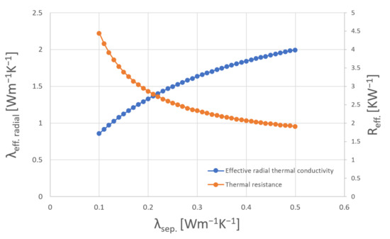
Figure 10.
Influence in varying thermal conductivity values of separator material on the effective thermal conductivity of a 18650 cylindrical cell.
Figure 10 shows that the effective radial thermal conductivity varies between 0.86 and 2 Wm−1·K−1 depending on the separator material. In comparison to the pipe method measurements, where the results vary between 0.51 and 0.73 Wm−1·K−1, the LFA and DSC based measurement results are much higher. A possible explanation is given in the simulation chapter where the temperature sensor position inside the cell is varied and an additional layer of air, indicating the possibility of missing thermal paste, is simulated.
3. Simulation
In this chapter, a simplified 2D-FEM-based model of a cylindrical cell is shown. The simulations were realized using FEMM (finite element method magnetics), version 4.2 by David Meeker [28]. To reduce computation time, only a cross section of a quarter circle was simulated, assuming axial symmetry of both axes. The heat flux on the outer surface of the cell and the heating wire temperature were defined as boundary conditions. The FEM tool automatically chooses the mesh size and density. For the following simulations the layer thickness and the measurement results from Table 5 and Table 6 were used. A thermal conductivity of Wm−1·K−1 was assumed for the separator layer. Therefore, the effective thermal conductivity of this simplified battery model is Wm−1·K−1, which can be calculated using Equation (2). The primary purpose of the simulation model is to determine the effects of an incorrectly assumed temperature sensor position. Furthermore, the effects of missing thermal paste between the temperature sensor and the bulk material of the cell are shown, as well as the influence of different heating wire positions on the calculation result. For this simplified model, the thickness of the anode, cathode and separator layer is calculated by summing up all the individual layer thicknesses in radial direction. Due to this simplification, no statement about the temperature distribution in the bulk material can be made. However, the core and the surface temperature of the cell can be simulated. Figure 11 shows the simulation model and the cross-section showing possible uncertainties. The simulation model contains a heat source in the center of the circle that represents the heating wire. A heat flux boundary condition on the outer surface of the cylinder is added to create similar conditions as in the measurements. With this boundary condition, a constant heat flow of 1.38 W is created. Different virtual measurement points (T1–T9) next to the heating wire are placed to represent the possible locations of the introduced temperature sensor as shown in Figure 11c.
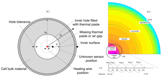
Figure 11.
Cross section of the cell (a) showing possible uncertainties that can influence the measurement results of the radial thermal conductivity. The simulation model (b) with virtual temperature sensors (T1–T9) and different positions (Pos.0–Pos.4) of the heating wire (c).
Using the results of these virtual temperature sensors leads to variations in the calculated radial thermal conductivity, shown in Figure 12. For this first simulation, the inner hole of the cell is completely filled with thermal paste. The thermal paste has a thermal conductivity of 5 Wm−1·K−1 to create the same conditions as in the pipe method. As shown in Figure 12 the closer the virtual sensor moves to the heating wire, the smaller the calculated effective thermal conductivity becomes. At a sensor distance of 1.7 mm to the inner surface the calculated thermal conductivity of the cell is 0.87 Wm−1·K−1, which is already a reduction of 25% compared to the given effective thermal conductivity of 1.17 Wm−1·K−1. For the second simulation an additional air gap was inserted between the sensor and the bulk material. This gap simulates the absence of thermal paste between the inner surface and the temperature sensor. The gap is varied between 10 µm to 100 µm, which is in the range of the thickness of a single separator layer and a negative electrode. Figure 12 also shows that a 50 µm air gap reduces the thermal conductivity to 0.56 Wm−1·K−1.
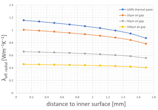
Figure 12.
Simulation results of different temperature sensor positions and missing thermal paste leading to wrong calculations.
These results lead to the conclusion that already a small space of 50 µm without thermal paste can cause large inaccuracies or variations in the radial thermal conductivity measurements. At this point the heating wire in the simulation model is located at the center of the cell, which is an ideal assumption. Therefore, additional simulations were performed, where the heating wire is moved stepwise from the central position to the inner surface of the cell. Figure 11c shows the different heating wire positions (Position 0 to Position 4). The heating wire is moved in 0.4 mm steps until the inner surface is reached. Each 0.2 mm, a virtual temperature sensor is placed, whose measurement results are taken to calculate the thermal conductivity. These calculation results and the possible error that can occur due to wrong assumptions are shown in Figure 13.
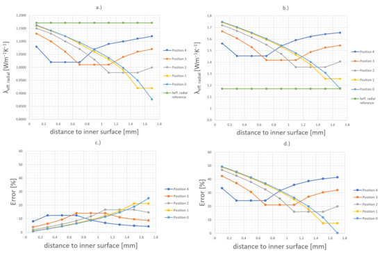
Figure 13.
Influence of different heating wire positions on the calculated thermal conductivity when the sensor position is unknown. The left side (a,c) shows the results when the thermal paste is not considered by using Equation (2). The right side (b,d) shows the results when the thermal paste is considered by using Equation (3).
Due to the unknown position of the heating wire and the temperature sensor, it is not possible to know how many layers should be considered in the calculation. In order to know whether a second layer should be taken into account, it is necessary to estimate the distance between the temperature sensor and the bulk material. If the thermal paste within the cell is taken into account, a misjudgment of the sensor position can lead to a larger error more quickly than if it is not taken into account, as can be seen in Figure 13b. In this case, a misjudgment leads to a significantly higher radial thermal conductivity. If the thermal paste is not taken into account, a misjudgment of the sensor position can lead to a lower radial thermal conductivity. Using Equation (2), which only considers one layer, leads to Figure 13a. Using the two-layer Equation (3) where the thermal conductivity of the first layer is 5 Wm−1·K−1, which is the conductivity of the used thermal paste, leads to an even higher deviation in the simulation results, as shown in Figure 13d.
4. Conclusions
This work analyzes the uncertainties of the pipe method when used for cylindrical LIB based effective radial thermal conductivity measurements. Two independent methods were used for this purpose. The first method, based on the pipe method, showed lower values for the thermal conductivity compared to the second approach which determines the effective radial thermal conductivity by measuring each layer type of the cell separately.
Due to the measurement setup of the pipe method, which can differ slightly from cell- to- cell, non-negligible tolerances can occur. The difficulties in sensor placement within the cell and the possibility of poor connection between the sensor and the bulk material, as well as other uncertainties, can lead to considerable tolerances. The type of temperature sensor must be also considered. Both sensors have their advantages and disadvantages. The FBGs are sensitive and small, and multiplexing is possible. The accuracies of the used sensors are ±1.5 C and ±0.8 C for the thermocouples and FBGs, respectively. However, influences such as strain and humidity can decrease the accuracy of the FBGs. This makes FBGs more difficult to handle than thermocouples. To show how these tolerances can affect the measurement, a simplified model was created with measurement results from the individual layers of the cell. It is important to mention that the simulation does not serve as a benchmark or reference for the first method, but it can be used to estimate the respective influences of the different measurement uncertainties. The simulation results of the model show that the results of the pipe method can be heavily influenced by an unknown position of the temperature sensor and the heating wire. The hole tolerance shown in Figure 11a and the possibility of missing or poorly distributed thermal paste, which leads to a higher thermal resistance between the sensor and the bulk surface, can also greatly influence the measurement results. The results also show that the separator has a major impact on the thermal conductivity.
A major disadvantage when measuring the thermal properties of the individual layers is that the cell structure must be known to calculate the effective thermal conductivity of the LIB. Furthermore, the influence of the thermal resistance from layer to layer is not taken into account with this method. Therefore, it must be considered in the subsequent calculation. As a result, the effective thermal conductivity can be lowered, depending on the assumption. With the help of these methods, an overall picture can be obtained, where the measurement of the individual layers, i.e., the second method, provides a more idealized result and thus represents an upper limit for the thermal conductivity. Conversely, the pipe method, due to the poor connection between the sensors and the bulk material, represents the lower limit of the radial thermal conductivity of the cell.
Furthermore, the effective radial thermal conductivity at three different SOC levels was measured, which increases slightly with increasing SOC. The authors of this work assume that due to the higher pressure in between the bulk material at higher SOC levels the thermal contact resistance between each layer decreases, which could result in a higher effective thermal conductivity.
In order to prevent possible uncertainties when using the pipe method, the positioning of the sensor and the heating wire should not be done manually. By positioning these with an automated process, measurement deviations between different cells that are caused by placement errors can be reduced and the comparability can be increased. Furthermore, it is important to minimize the possible contact resistance between the temperature sensor and the heating wire as well as the bulk material. The reference measurements showed that the literature values are most accurately achieved if the entire inner hole of the cylinder is filled with thermal paste. When a heat flux sensor is used to measure the heat flow through the bulk material, it is important to consider the area of the insulation material in the calculation. The tolerances of the bulk material, which cause a variable inner radius of the cell, should also be considered.
Author Contributions
M.K., J.U., D.L. and G.G. performed the experiments; M.K., D.L. and H.P. conceived and designed the experiments; M.K, J.U. and D.L. analyzed the data; M.K. and H.P. conceptualized the manuscript; M.K. performed overall writing of the manuscript; J.U. wrote the FBG section; H.P. partially wrote the abstract, introduction and measurement section; A.B. and H.P. took charge of scientific supervision. All authors have read and agreed to the published version of the manuscript.
Funding
This work received funding from the Austrian Research Promotion Agency (FFG) within the collaborative project MOGLI (Grant Agreement No. 879610).
Institutional Review Board Statement
Not applicable.
Informed Consent Statement
Not applicable.
Data Availability Statement
Data are available upon request from the corresponding author.
Acknowledgments
The authors would like to thank all our colleagues from AIT Austrian Institute of Technology and Graz University of Technology for the perfect support and the good teamwork.
Conflicts of Interest
The authors declare no conflict of interest.
Abbreviations
The following abbreviations are used in this manuscript:
| BMS | Battery management system |
| CT | Computed tomography |
| DSC | Differential scanning calorimetry |
| FBG | Fiber Bragg grating |
| FEM | Finite element method |
| HFM | Heat flow meter |
| LFA | Laser flash method |
| LIB | Lithium-ion secondary battery |
| NCA | Nickel cobalt aluminium oxide |
| PMMA | Polymethylmethacrylate |
| SOC | State of charge |
| Thermal conductivity (Wm−1·K−1) | |
| Heat flow (W) | |
| Heat flux density (W/m2) | |
| Temperature difference (C) | |
| A | Surface area of the specimen (m2) |
| a | Thermal diffusivity (m2/s) |
| Density (kg·m−3) | |
| Heat capacity (J/K) | |
| Thermal resistance (K/W) | |
| Outer radius (m) | |
| Inner radius (m) | |
| Sensor radius (m) | |
| Surface area of cell without top and bottom area (m2) |
References
- Stampatori, D.; Raimondi, P.P.; Noussan, M. Li-Ion Batteries: A Review of a Key Technology for Transport Decarbonization. Energies 2020, 13, 2638. [Google Scholar] [CrossRef]
- Cerdas, F.; Titscher, P.; Bognar, N.; Schmuch, R.; Winter, M.; Kwade, A.; Herrmann, C. Exploring the Effect of Increased Energy Density on the Environmental Impacts of Traction Batteries: A Comparison of Energy Optimized Lithium-Ion and Lithium-Sulfur Batteries for Mobility Applications. Energies 2018, 11, 150. [Google Scholar] [CrossRef] [Green Version]
- Kim, Y.; Siegel, J.B.; Stefanopoulou, A.G. A computationally efficient thermal model of cylindrical battery cells for the estimation of radially distributed temperatures. In Proceedings of the 2013 American Control Conference, Washington, DC, USA, 17–19 June 2013; pp. 698–703. [Google Scholar] [CrossRef]
- Wang, Z.; Ma, J.; Zhang, L. Finite Element Thermal Model and Simulation for a Cylindrical Li-Ion Battery. IEEE Access 2017, 5, 15372–15379. [Google Scholar] [CrossRef]
- Guo, M.; White, R.E. Mathematical model for a spirally-wound lithium-ion cell. J. Power Sources 2014, 250, 220–235. [Google Scholar] [CrossRef]
- Wei, Z.; Zhao, J.; He, H.; Ding, G.; Cui, H.; Liu, L. Future smart battery and management: Advanced sensing from external to embedded multi-dimensional measurement. J. Power Sources 2021, 489, 229462. [Google Scholar] [CrossRef]
- Isothermal Battery Calorimeter Cell Format: Cylindrical. Available online: https://www.thermalhazardtechnology.com/battery-products/isothermal-battery-calorimeter (accessed on 22 December 2021).
- Drake, S.; Wetz, D.; Ostanek, J.; Miller, S.; Heinzel, J.; Jain, A. Measurement of anisotropic thermophysical properties of cylindrical Li-ion cells. J. Power Sources 2014, 252, 298–304. [Google Scholar] [CrossRef]
- Yang, Y.; Huang, X.; Cao, Z.; Chen, G. Thermally conductive separator with hierarchical nano/microstructures for improving thermal management of batteries. Nano Energy 2016, 22, 301–309. [Google Scholar] [CrossRef] [Green Version]
- Bhundiya, H. Radial Thermal Conductivity Measurements of Lithium-Ion Battery Cells. Available online: https://curj.caltech.edu/2020/06/20/radial-thermal-conductivity-measurements-of-lithium-ion-battery-cells/r (accessed on 7 February 2022).
- Tousi, M.; Sarchami, A.; Kiani, M.; Najafi, M.; Houshfar, E. Numerical study of novel liquid-cooled thermal management system for cylindrical Li-ion battery packs under high discharge rate based on AgO nanofluid and copper sheath. J. Energy Storage 2021, 41, 102910. [Google Scholar] [CrossRef]
- Al-Zareer, M.; Michalak, A.; Da Silva, C.; Amon, C.H. Predicting specific heat capacity and directional thermal conductivities of cylindrical lithium-ion batteries: A combined experimental and simulation framework. Appl. Therm. Eng. 2021, 182, 116075. [Google Scholar] [CrossRef]
- Keil, P.; Rumpf, K.; Jossen, A. Thermal impedance spectroscopy for Li-ion batteries with an IR temperature sensor system. In Proceedings of the 2013 World Electric Vehicle Symposium and Exhibition (EVS27), Barcelona, Spain, 17–20 November 2013; pp. 1–11. [Google Scholar] [CrossRef] [Green Version]
- Oehler, D.; Bender, J.; Seegert, P.; Wetzel, T. Investigation of the Effective Thermal Conductivity of Cell Stacks of Li-Ion Batteries. Energy Technol. 2021, 9, 2000722. [Google Scholar] [CrossRef]
- Maleki, H.; Al-Hallaj, S.; Selman, J.; Dinwiddie, R.; Wang, H. Thermal Properties of Lithium-Ion Battery and Components. J. Electrochem. Soc. 1999, 146, 947–954. [Google Scholar] [CrossRef]
- Muratori, M. Thermal Characterization of Lithium-Ion Battery Cell. Ph.D. Thesis, Politecnico Di Milano, Milano, Italy, 2008. [Google Scholar]
- Chen, S.C.; Wang, Y.Y.; Wan, C.C. Thermal Analysis of Spirally Wound Lithium Batteries. J. Electrochem. Soc. 2006, 153, A637. [Google Scholar] [CrossRef]
- Al-Ajlan, S.A. Measurements of thermal properties of insulation materials by using transient plane source technique. Appl. Therm. Eng. 2006, 26, 2184–2191. [Google Scholar] [CrossRef]
- Yüksel, N. The Review of Some Commonly Used Methods and Techniques to Measure the Thermal Conductivity of Insulation Materials; IntechOpen: London, UK, 2016; Available online: https://www.intechopen.com/chapters/51497 (accessed on 7 February 2022).
- Parker, W.J. Flash Method of Determining Thermal Diffusivity, Heat Capacity, and Thermal Conductivity. J. Appl. Phys. 1961, 32, 1679–1684. [Google Scholar] [CrossRef]
- Matteo, L. Characterizing the Measurement Uncertainty of a High-Temperature Heat Flux Differential Scanning Calorimeter. Master’s Thesis, TU-Graz, Graz, Austria, 2014. [Google Scholar]
- Popp, H.; Koller, M.; Jahn, M.; Bergmann, A. Mechanical methods for state determination of Lithium-Ion secondary batteries: A review. J. Energy Storage 2020, 32, 101859. [Google Scholar] [CrossRef]
- Oh, K.Y.; Epureanu, B.I. A novel thermal swelling model for a rechargeable lithium-ion battery cell. J. Power Sources 2016, 303, 86–96. [Google Scholar] [CrossRef] [Green Version]
- Grimsmann, F.; Brauchle, F.; Gerbert, T.; Gruhle, A.; Knipper, M.; Parisi, J. Hysteresis and current dependence of the thickness change of lithium-ion cells with graphite anode. J. Energy Storage 2017, 12, 132–137. [Google Scholar] [CrossRef]
- Hemmerling, J.; Guhathakurta, J.; Dettinger, F.; Fill, A.; Birke, K.P. Non-Uniform Circumferential Expansion of Cylindrical Li-Ion Cells—The Potato Effect. Batteries 2021, 7, 61. [Google Scholar] [CrossRef]
- Willenberg, L.K.; Dechent, P.; Fuchs, G.; Sauer, D.U.; Figgemeier, E. High-Precision Monitoring of Volume Change of Commercial Lithium-Ion Batteries by Using Strain Gauges. Sustainability 2020, 12, 557. [Google Scholar] [CrossRef] [Green Version]
- University, W.S. Steady Heat Condition. 2021. Available online: http://cecs.wright.edu/~sthomas/htchapter03.pdf (accessed on 7 February 2022).
- Finite Element Method Magnetics: HomePage. Available online: https://www.femm.info/wiki/HomePage (accessed on 21 December 2021).
Publisher’s Note: MDPI stays neutral with regard to jurisdictional claims in published maps and institutional affiliations. |
© 2022 by the authors. Licensee MDPI, Basel, Switzerland. This article is an open access article distributed under the terms and conditions of the Creative Commons Attribution (CC BY) license (https://creativecommons.org/licenses/by/4.0/).