Quantitative Design for the Battery Equalizing Charge/Discharge Controller of the Photovoltaic Energy Storage System

Abstract

The purpose of this paper is to develop a photovoltaic module array with an energy storage system that has equalizing charge/discharge controls for regulating the power supply to the grid. Firstly, the boost converter is used in conjunction with maximum power point tracking (MPPT) such that the photovoltaic module array (PVMA) can output maximum power at any time. The battery equalizing charge/discharge architecture is composed of multiple sets of bidirectional buck–boost soft-switching converters in serial connection in order to achieve zero-voltage switching (ZVS) and zero-current switching (ZCS) so that when the charge/discharge power is above 150 W, the converter efficiency can be increased by 3%. The voltage and current signals from the battery are captured and input into the digital signal processor (DSP) to establish an equalizing charge/discharge control rule. For the output voltage control of the bidirectional buck–boost soft-switching converter, the dynamic mode is derived by first using the step response at chosen operating point, then quantitatively designing the controller parameters for the converter, so that the output voltage response can meet the pre-defined performance specifications. Finally, actual test results prove that the equalizing charge/discharge time of the quantitative design controller is shortened by more than 10% when compared to the traditional proportional-integral (P-I) controller regardless of charging or discharging; this also proves that the design of the photovoltaic module array with an energy storage system (ESS) that has equalizing charge/discharge controls is valid.

1. Introduction

Currently, power from most photovoltaic module arrays (PVMAs) is connected directly to the power company’s power grid after being converted from DC to AC by the inverter, thereby achieving maximum economic benefits. However, photovoltaic power generation is not a stable source of power and is easily affected by factors such as environmental changes and the amount of sunlight [1]. The drastic changes in its output can cause deviations in the voltage and frequency of the grid system, and thus has a significant impact on the quality of power from the grid. By building microgrids, the burden on the grid can be reduced. Microgrids are small-scale power grids that are combined with renewable energy [2], among which, photovoltaic energy is the most common source of power in microgrids [3,4], furthermore, microgrid systems are able to operate independently. Nonetheless, photovoltaic power generation efficiency is affected by changes in the weather, leading to unstable energy generation. Thus, to regulate power, an energy storage battery system must be used for photovoltaic power generation to store the excess energy in the battery [5]. Then, when the microgrid is unable to produce sufficient power, the battery can be used as an auxiliary power supply, so that the microgrid can obtain greater economic benefits while solving the problem of unstable power supply quality from the grid under high renewable energy proportions.

The energy storage system for photovoltaic power generation can regulate the power via the bidirectional buck–boost converter to provide stable DC-link voltage output [6]. Since the output power from photovoltaic energy changes due to changing amount of sunlight, in order to maintain the DC-link voltage at a set value, the controller parameters for the bidirectional buck–boost converter must be designed properly so that the converter will have good output performance. The architecture of the commonly adopted traditional P-I controller is simple and does not require complex calculations, but the controller parameters can only be adjusted through the trial-and-error method, thus requiring more time to obtain the controller parameters [6,7,8]. Furthermore, whereas the controller designed using the Bode plot can obtain the controller parameters quickly but does not take the converter’s dynamic characteristic of wide operating spectrum into consideration, and thus is only able to obtain the dynamic response under certain conditions; once the operating point changes, the system will be unable to operate under the better performance response [9,10]. For other existing intelligent controllers such as the particle swarm optimization (PSO) [11,12], genetic algorithm (GA) [13,14], sliding mode control [15,16], fuzzy control [17,18,19], and neural network [20], although these above controllers can all incorporate the traditional P-I controller into the design, the calculation process for these intelligent algorithms are complex, leading to difficulty in obtaining the design parameters, and is also more difficult to implement in actual application.

For these reasons, this paper will carry out the quantitative design of the DC bus voltage controller for the bidirectional buck–boost soft-switching converter [21,22]. The controller parameters designed will enable the battery to reach charge equalization quickly, and when used with the photovoltaic power generation system, the battery can store energy and become an auxiliary power supply, thereby stabilizing the DC-link voltage. The overall architecture is shown in Figure 1. The power output of the PVMA changes along with the amount of sunlight, so the perturb and observe method (P&O) [23,24] needs to be used to maintain the output power at the maximum power point (MPP) by incorporating the boost converter. For the equalizing charge/discharge architecture adopted in this paper, it is composed of multiple sets of bidirectional buck–boost soft-switching converters [21,22] in serial connection, using the sensor circuit to send the voltage and current of the maximum power point tracker (MPPT) and equalizing charge/discharge circuit back to digital signal processor (DSP)TMS320F2809 [25] for calculation. At the same time, we established an equalizing charge/discharge rule to limit the battery’s maximum charge/discharge current to prevent battery damage from over-current and validate the feasibility of the adopted equalizing charge/discharge architecture through an actual test. Lastly, we designed the controller for the bidirectional buck–boost soft-switching converter through quantitative methods so the voltage response output by the converter can meet defined specifications and compared it with the charge/discharge speed of the traditional P-I controller.

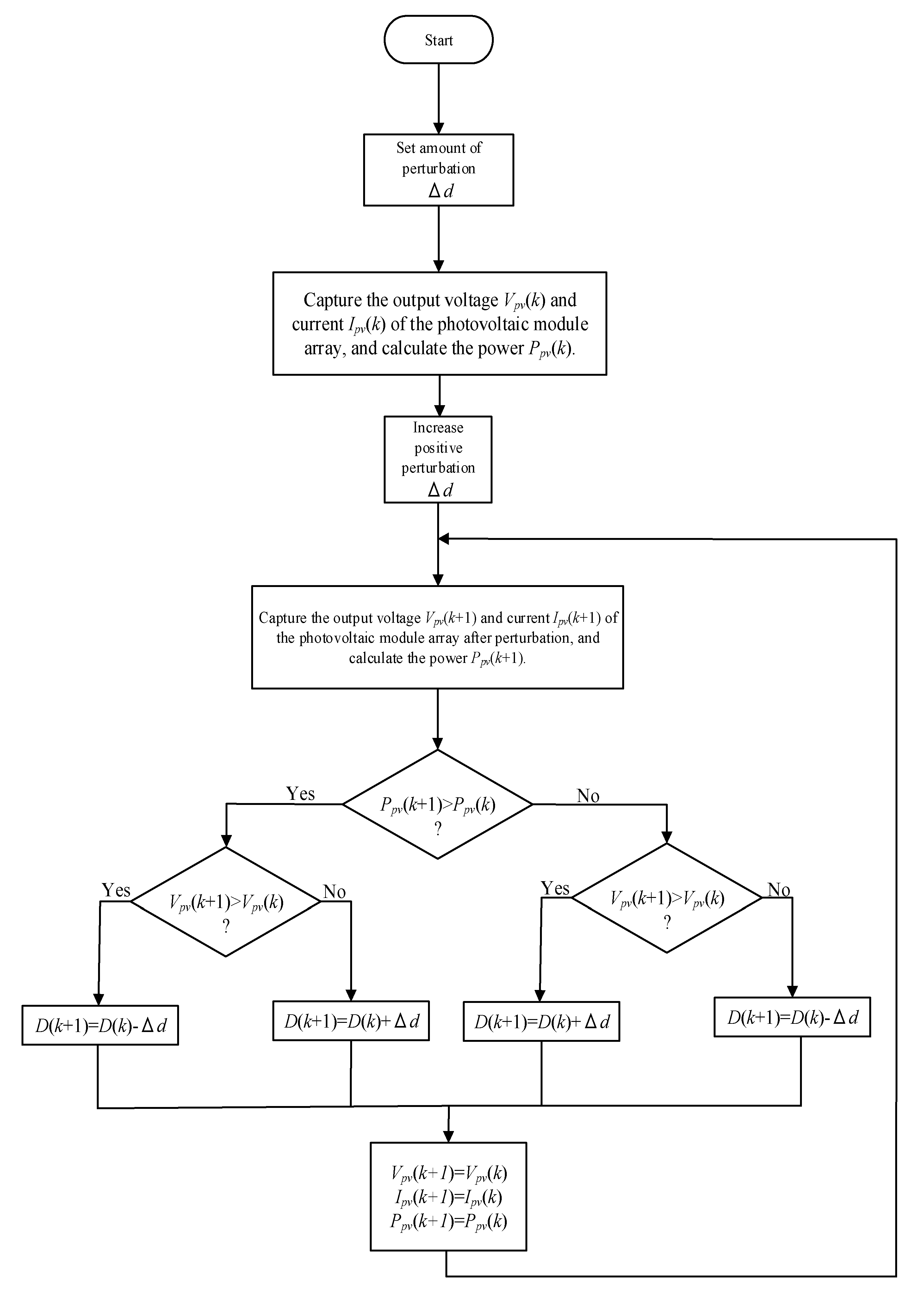
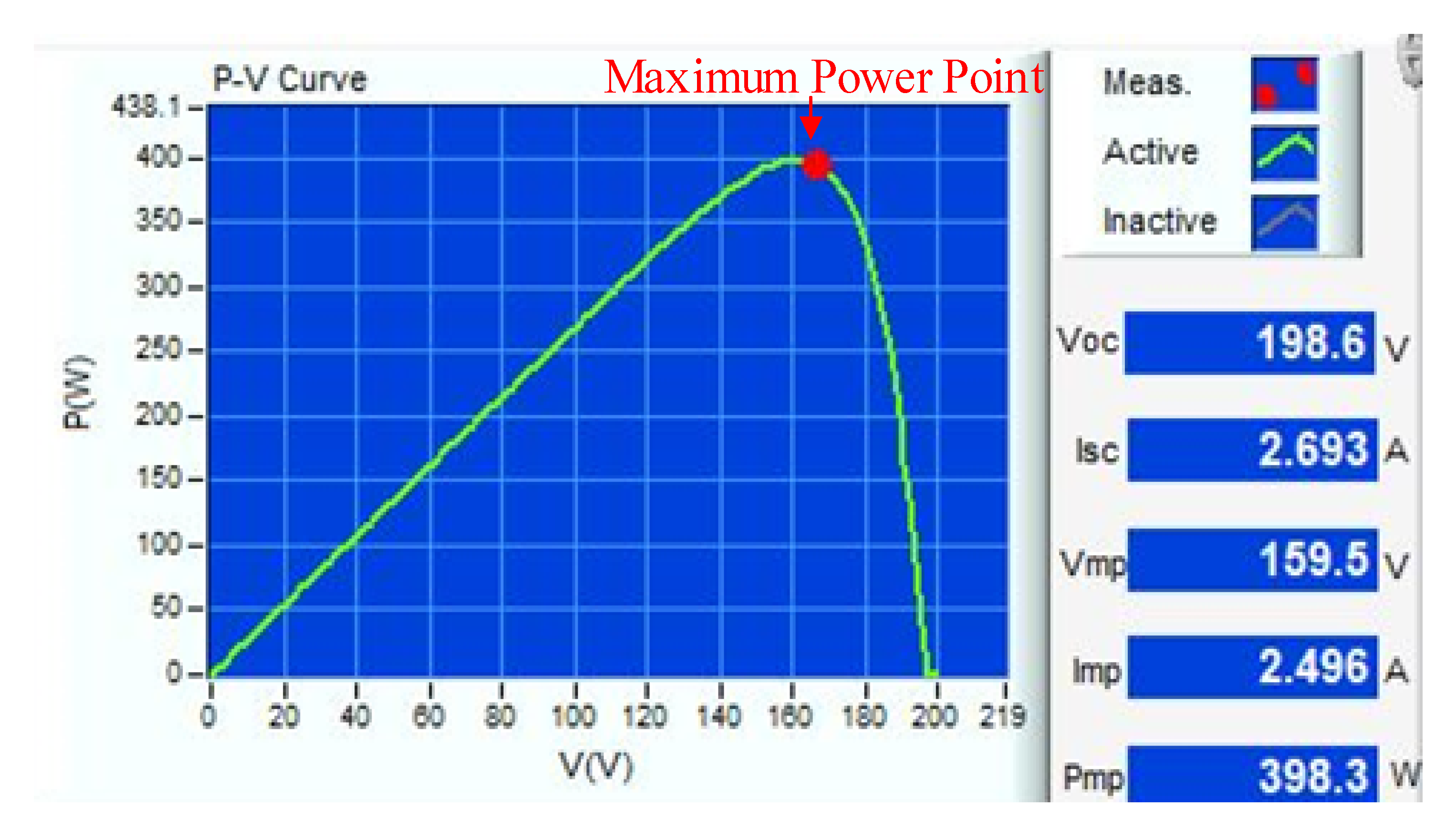
2. The Adopted MPPT Method

The perturb and observe (P&O) MPPT method compares the current output power against the output power before perturbation and determines the direction of the next perturbation. If the current output power of the PVMA is higher than the power before perturbation, the perturbation will continue in the same direction; conversely, if the current output power of the PVMA is lower than the power before perturbation, then the direction of the next perturbation will change to achieve MPPT. Since there are few parameters requiring measurement and due to the simple architecture, the P&O MPPT method has become the most commonly used method; its perturbation process is shown in Figure 2 [23,24].

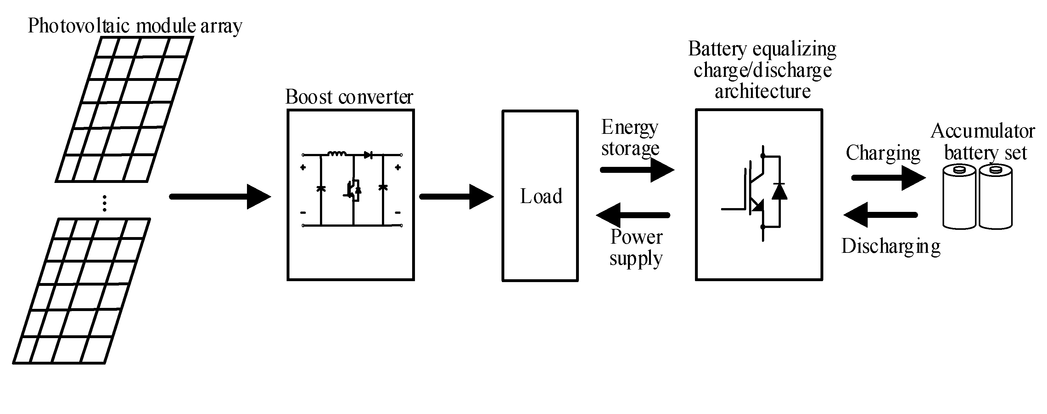
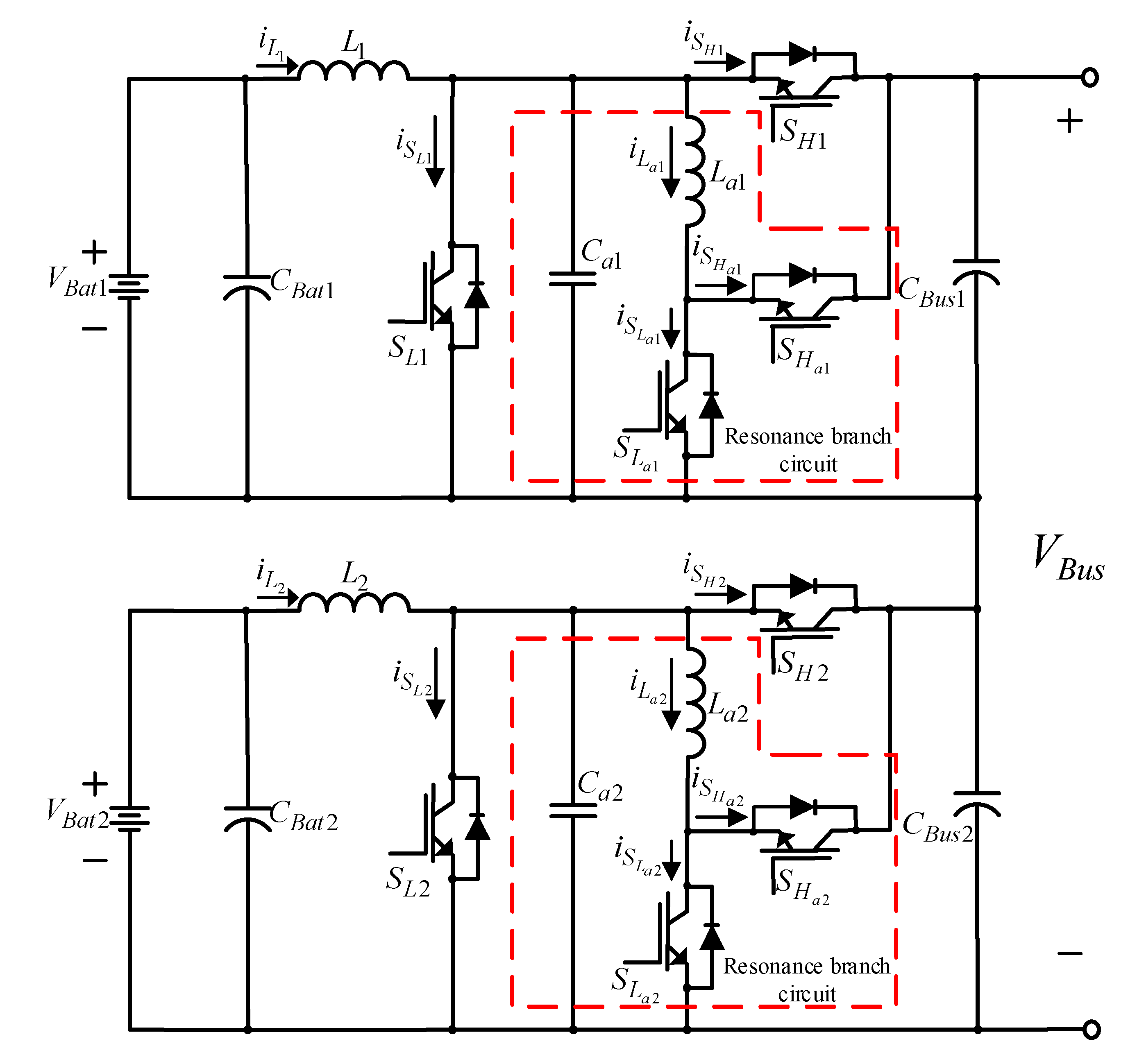
3. The Adopted Equalizing Charge/Discharge Architecture

As the condition of each battery is different, when multiple sets of serial-connected batteries are charging/discharging, it can lead to conditions of over-charge and over-discharge. To solve this problem, this paper serial-connects two sets of bidirectional buck–boost soft-switching converters [21,22] into equalizing charge/discharge architecture to carry out equalizing charge/discharge control of two sets of serial-connected batteries. The circuit layout is shown in Figure 3, and the electrical specifications and component parameters of the equalizing charge/discharge architecture are compiled separately into

Table 1. The electrical specifications of the bidirectional buck–boost soft-switching converter.

Parameters	Specifications
Voltage at high-voltage side(VBus)	240 V
Voltage of first battery set at low-voltage side (VBat1)	12 V
Voltage of second battery set at low-voltage side (VBat2)	12 V
Switching frequency (f)	25 kHz
Maximum operating power (Pmax)	300 W
Voltage ripple at high-voltage side (ΔVBus,ripple)	0.5%
Voltage ripple at low-voltage side (ΔVBat,ripple)	0.5%

and

Table 2. The component parameters of the bidirectional buck–boost soft-switching converter.

Component Name	Specifications
Main inductor (L1, L2)	1.425 mH
Resonance inductor (La1, La2)	18 μH
Capacitor at high-/low-voltage side (CBat1, CBat2, CBus1, CBus2)	270 μF/450 V
Main switch and auxiliary switch	IGBT-IXGH48N60C3D1 (600 V/48 A)

[22]. The component parameters of the bidirectional buck–boost soft-switching converter listed in Table 2 are derived in [22]. This architecture is composed of multiple sets of serial-connected bidirectional buck–boost soft-switching converters; its pulse width modulation (PWM) control signal first conducts the auxiliary switch, enabling resonance from the resonance inductor and resonance capacitor, then the main switch is activated, which carries out the energy transfer of the serial-connected battery set, thereby achieving equalizing charge/discharge [22].

The equalizing charge/discharge architecture adopted in this paper enables the individual charge/discharge of each battery to achieve the goal of equalizing charge/discharge; this architecture can effectively limit the charge/discharge current, thereby reducing the problem of battery degradation. Lead-acid batteries are the storage battery type commonly seen in the commercial market because they are designed with the following advantages: lower cost, better stability and wider working temperature range, etc. Being easily accessible, lead-acid batteries are used in this paper as the research target. Attributing to the development of innovative battery structure and materials in recent years, the performance of the conventional lead-acid battery has also been significantly improved. The batteries used in this paper are lead-acid batteries; therefore, the limit of the charge/discharge current is set to 0.3 C to extend the battery life [26]. This architecture adopted the digital signal processor TMS320F2809 as the control core, and the voltage and current signals are sent back to the digital signal processor through the sensor for calculations, then, through the quantitatively designed equalizing charge/discharge controller, outputs the corresponding pulse width modulation (PWM) control signal. Before initiating the charge/discharge control, the photovoltaic power generation conditions must first be evaluated before deciding on the mode of charge/discharge. If the power generated from photovoltaic energy is greater than the load demand, then the charging of the battery can be equalized; on the other hand, if the power generated from photovoltaic energy is lower than the load demand, then the discharging control of the battery can be equalized to act as an auxiliary power supply to the load end.

The soft switching converter selected for this experiment is equipped with a resonant circuit for executing the resonance process before energizing the high-voltage/low-voltage (HV/LV) main switches (S_H1, S_H2, S_L1 and S_L2) to obtain the characteristics required for zero-voltage switching (ZVS) and zero-current switching (ZCS). Therefore, when using the soft switching function, the converter must be operated under heavy load conditions to achieve higher conversion efficiency. When operating under a lighter load (under 150 W), because the inductive current is under the discontinuous conduction mode, it may prevent the resonance circuit from smoothly executing the resonance. As a result, limited efficiency can be noted for the soft switching converter only, and the efficiency will become even lower than the conventional hard switching converter.

4. Quantitative Design of the Bidirectional Buck–Boost Soft-Switching Converter Controller

The equalizing charge/discharge controls of the traditional P-I controller are simple and do not require complex calculations, but the controller parameters can only be adjusted through the trial-and-error method, thus requiring more time to obtain the controller parameters. Furthermore, good control performance cannot be obtained under different operating points. In order for the battery equalizing charge/discharge control to achieve good control performance under various operating conditions, the quantitative design [27] of the controller parameters for the bidirectional buck–boost soft-switching converter is adopted such that the output voltage response can meet the defined performance specifications, and through the controls of the controller, the battery equalizing charge/discharge speed response can be increased.

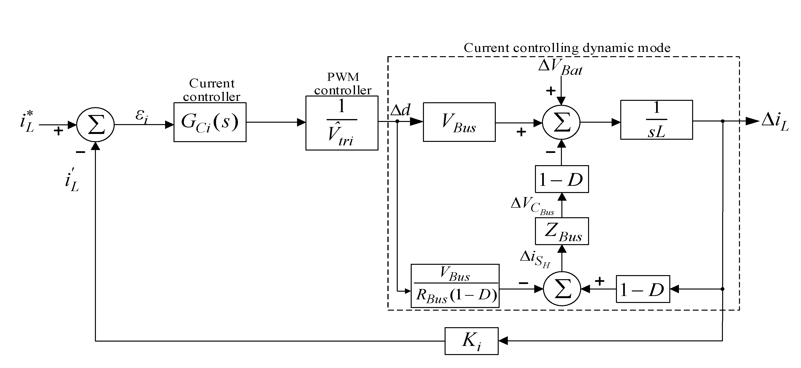
4.1. Quantitative Design of the Current Controller

The current controller for the bidirectional buck–boost soft-switching converter is designed so that the converter can operate under the current continuous conducting mode. Compared to the whole switching period, the auxiliary branch switching time for the bidirectional buck–boost soft-switching converter is comparatively shorter; therefore during the dynamic mode analysis process, the auxiliary branch switching time can be omitted [6,21,22]. In addition, since the main switches of the converter S_L and S_H are complementarily controlled, the results derived from both the boost mode or the buck mode are the same; therefore, the analysis process below is derived from the dynamic mode of the converter only under the boost mode.

In order to ensure that Equation (1) meets the requirements regardless of a light load or heavy load, the maximum value of the inductor current I_L—that is, the peak value of i_L at full load ${({\widehat{I}}_L)}_{\mathit{max}}$ is used to determine the on-time $t_D$ of the auxiliary switch, and $t_D$ is usually 5~10% of the switching period T [6]. In addition, a margin time $t_{\epsilon }$ is required to obtain a reliable t_D, so here, we set $t_D$ = 0.1 T = 4 µs, and $t_{\epsilon }$ = 0.01 T = 0.4 μs, and then used Equation (1) to derive a maximum resonance inductance value L_a1 = L_a2 = 18 μH, so we can select a resonance inductance value smaller than 18μH, which would be acceptable. In addition, the selected switching component IGBT-IXGH48N60C3D1 has a stray capacitance of 202pF, so the resonance capacitors C_a1 and C_a2 can be replaced by stray capacitors:

$$\begin{array}{ll}{t}_d& =t_D+t_{\epsilon }\\ & =\frac{{\widehat{I}}_{{}_{Lm}}}{V_H}{L}_r+\frac{\pi }{\mathit{2}}\sqrt{L_a{C}_a}+t_{\epsilon }\end{array}$$

(1)

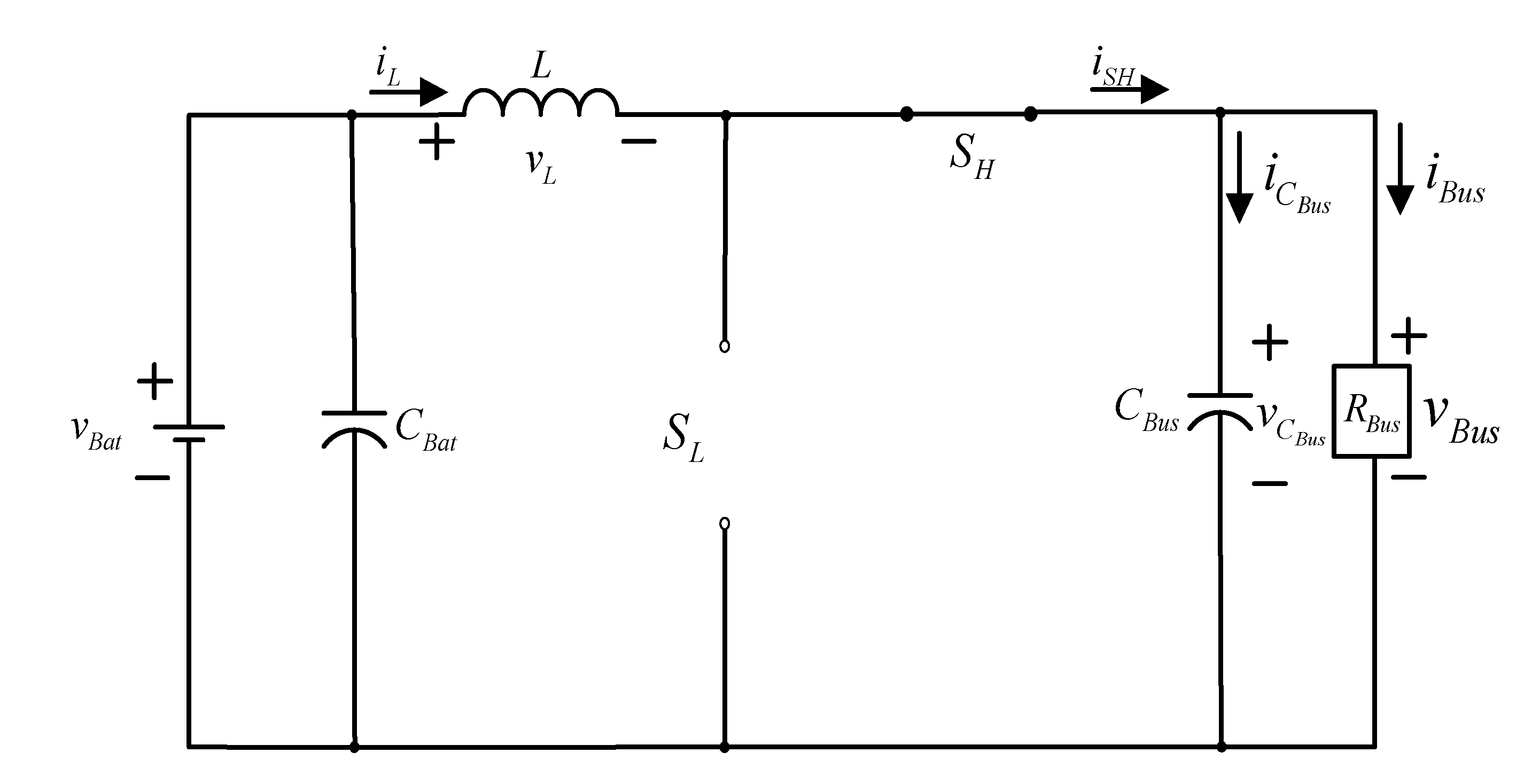
4.1.1. Conducting State of Low-Voltage Side Switch S_L ($0\le t\le dT$)

When the low-voltage side switch S_L is conducting, the high-voltage side switch S_H is in a cut-off state at this time; the equivalent circuit is shown in Figure 4. The state equation for the converter can be represented by:

$$\left\{\begin{array}{l}\frac{d}{dt}\left[\begin{array}{l}{i}_L\\ v_{C_{Bus}}\end{array}\right]=\left[\begin{array}{cc}0& 0\\ 0& -\frac{1}{C_{Bus}{R}_{Bus}}\end{array}\right]\left[\begin{array}{l}{i}_L\\ v_{C_{Bus}}\end{array}\right]+\left[\begin{array}{c}\frac{1}{L}\\ 0\end{array}\right]v_{Bat}\\ v_{Bus}=\left[\begin{array}{ll}0\hfill & 1\hfill \end{array}\right]\left[\begin{array}{l}{i}_L\\ v_{C_{Bus}}\end{array}\right]{,}_{}{i}_{S_H}=0\end{array}\right.$$

(2)

4.1.2. Cut-Off State of Low-Voltage Side Switch S_L ($dT\le t\le T$)

When the low-voltage side switch S_L is in a cut-off state, the high-voltage side switch S_H is conducting; the equivalent circuit can be presented in Figure 5. The load in the equivalent circuit is pure resistance R_Bus. Then, the state equation can be obtained in Equation (3).

$$\left\{\begin{array}{l}\frac{d}{dt}\left[\begin{array}{l}{i}_L\\ v_{C_{Bus}}\end{array}\right]=\left[\begin{array}{cc}0& -\frac{1}{L}\\ \frac{1}{C_{Bus}}& -\frac{1}{C_{Bus}{R}_{Bus}}\end{array}\right]\left[\begin{array}{l}{i}_L\\ v_{C_{Bus}}\end{array}\right]+\left[\begin{array}{c}\frac{1}{L}\\ 0\end{array}\right]v_{Bat}\\ v_{Bus}=\left[\begin{array}{ll}0\hfill & 1\hfill \end{array}\right]\left[\begin{array}{l}{i}_L\\ v_{C_{Bus}}\end{array}\right]{,}_{}{i}_{S_H}=i_L\end{array}\right.$$

(3)

Then, the state space averaging method is used on the state equation for the switch S_L to obtain the average over one period, where Equation (2) is multiplied by dT, plus Equation (3) multiplied by (1 − d) T and divided by T, to arrive at:

$$\left\{\begin{array}{l}\frac{d}{dt}\left[\begin{array}{l}{i}_L\\ v_{C_{Bus}}\end{array}\right]=\left[\begin{array}{cc}0& -\frac{(1-d)}{L}\\ \frac{(1-d)}{C_{Bus}}& -\frac{1}{C_{Bus}{R}_{Bus}}\end{array}\right]\left[\begin{array}{l}{i}_L\\ v_{C_{Bus}}\end{array}\right]+\left[\begin{array}{c}\frac{1}{L}\\ 0\end{array}\right]v_{Bat}\\ v_{Bus}=\left[\begin{array}{ll}0\hfill & 1\hfill \end{array}\right]\left[\begin{array}{l}{i}_L\\ v_{C_{Bus}}\end{array}\right]{,}_{}{i}_{S_H}=(1-d)i_L\end{array}\right.$$

(4)

Equation (4) is a nonlinear equation; to linearize Equation (4), the perturbation signal is added to the operating point to make $v_{Bat}=V_{Bat}+\Delta v_{Bat}$, $v_{C_{Bus}}=V_{C_{Bus}}+\Delta v_{C_{Bus}}$, $v_{Bus}=V_{\mathrm{Bus}}+\Delta v_{Bus}$, $i_L=I_L+\Delta i_L$, $i_{S_H}=I_{S_H}+\Delta i_{S_H}$ and duty cycle $d=D+\Delta d$, where V_Bat, ${\mathrm{V}}_{C_{Bus}}$, V_Bus, I_L, $I_{S_H}$ and D are the values for the respective operating points; the perturbation signal is then substituted into Equation (4) to arrive at Equation (5) after rearrangement.

$$\left\{\begin{array}{l}\frac{d}{dt}\left[\begin{array}{l}{I}_L+\mathrm{\Delta }{i}_L\\ V_{C_{Bus}}+\mathrm{\Delta }{v}_{C_{Bus}}\end{array}\right]=\left[\begin{array}{cc}0& -\frac{\left[1-(D+\mathrm{\Delta }d)\right]}{L}\\ \frac{[1-(D+\mathrm{\Delta }d)]}{C_{Bus}}& -\frac{1}{C_{Bus}{R}_{Bus}}\end{array}\right]\left[\begin{array}{l}{I}_L+\mathrm{\Delta }{i}_L\\ V_{C_{Bus}}+\mathrm{\Delta }{v}_{C_{Bus}}\end{array}\right]\\ +\left[\begin{array}{c}\frac{1}{L}\\ 0\end{array}\right](V_{\mathit{Bat}}+\mathrm{\Delta }{v}_{Bat})\\ V_{Bus}+\mathrm{\Delta }{v}_{Bus}=\left[\begin{array}{ll}0\hfill & 1\hfill \end{array}\right]{\left[\begin{array}{l}{I}_L+\mathrm{\Delta }{i}_L\\ V_{C_{Bus}}+\mathrm{\Delta }{v}_{C_{Bus}}\end{array}\right]}_{}\\ I_{S_H}+\mathrm{\Delta }{i}_{S_H}=\left[1-(D+\mathrm{\Delta }d)\right](I_L+\mathrm{\Delta }{i}_L)\end{array}\right.$$

(5)

Equation (5) is divided into two parts: the steady state and dynamic state—they are analyzed below.

4.1.3. Steady State

The differential item and perturbation amount of Equation (5) must be set to zero, and the steady-state equation of the operating point after the transpositioning rearrangement can be obtained with the following:

$$\left\{\begin{array}{l}{V}_{Bat}=(1-D)V_{C_{Bus}}\\ V_{Bus}=V_{C_{Bus}}=(1-D)I_L{R}_{Bus}\\ I_{S_H}=\frac{V_{Bus}}{R_{Bus}}=(1-D)I_L\end{array}\right.$$

(6)

4.1.4. Dynamic State

From Equation (4), the equation for small perturbation signal of the operating points (I_L, V_Bus, $I_{S_H}$, D, $V_{C_{Bus}}$) is:

$$\left\{\begin{array}{l}\frac{d\Delta i_L}{dt}=-\frac{(1-D)}{L}\Delta v_{C_{Bus}}+\frac{1}{L}\Delta v_{Bat}+\frac{V_{C_{Bus}}}{L}\Delta d\\ \frac{d\Delta v_{C_{Bus}}}{dt}=\frac{(1-D)}{C_{Bus}}\Delta i_L-\frac{1}{R_{Bus}{C}_{Bus}}\Delta v_{C_{Bus}}-\frac{I_L}{C_{Bus}}\Delta d\\ \Delta v_{Bus}=\Delta v_{C_{Bus}}\\ \Delta i_{S_H}=(1-D)\Delta i_L-I_L\Delta d\end{array}\right.$$

(7)

In order to deduce the transfer function of the state equation, Laplace transformation on Equation (7) must be performed to obtain Equations (8)–(11), then the above equation can be used to draw the block diagram containing the current controlling dynamic mode as shown in Figure 6.

$$\Delta i_L(s)=\frac{-(1-D)}{sL}\Delta v_{C_{Bus}}(s)+\frac{1}{sL}\Delta v_{Bat}(s)+\frac{V_{C_{Bus}}}{sL}\Delta d(s)$$

(8)

$$\begin{array}{ll}\Delta v_{C_{Bus}}\left(s\right)& =\frac{\left(1-D\right)}{C_{Bus}s}\Delta i_L\left(s\right)-\frac{1}{R_{Bus}{C}_{Bus}s}\Delta v_{C_{Bus}}\left(s\right)-\frac{I_L}{C_{Bus}s}\Delta d\left(s\right)\hspace{0.33em}\\ & =Z_{Bus}(s)\left[\left(1-D\right)\Delta i_L\left(s\right)-I_L\hspace{0.33em}\Delta d\left(s\right)\right]\end{array}$$

(9)

$$\begin{array}{ll}\Delta i_{S_H}\left(s\right)& =\left(1-D\right)\Delta i_L\left(s\right)-I_L\Delta d\left(s\right)\hspace{0.33em}\\ & =\left(1-D\right)\Delta i_L\left(s\right)-\frac{V_{Bus}}{R_{Bus}\left(1-D\right)}\hspace{0.33em}\Delta d\left(s\right)\end{array}$$

(10)

where:

$$Z_{\mathit{Bus}}(s)=\frac{R_{Bus}}{1+R_{Bus}{C}_{Bus}s}$$

(11)

The transfer function $\frac{\Delta i_L(s)}{\Delta d(s)}\left|\begin{array}{l}\\ {}_{\Delta v_{Bat}(s)=0}\end{array}\right.$ in Figure 4 can be derived from Equation (7), where Equation (7) is re-written into the transfer function in Equation (12):

$$\frac{\Delta i_L\left(s\right)}{\Delta d\left(s\right)}\left|\begin{array}{l}\\ {}_{\Delta v_{Bat}\left(s\right)=0}\end{array}\right.=\frac{R_{Bus}L{V}_{Bus}s+2V_{Bus}}{R_{Bus}L{C}_{Bus}{s}^2+Ls+{(1-D)}^2{R}_{Bus}}$$

(12)

The current loop gain transfer function LG(s) can be derived from Equation (12) and Figure 6 as shown in Equation (13):

$$LG(s)=\frac{G_{ci}(s)\frac{1}{{\widehat{V}}_{tri}}{K}_i(R_{Bus}L{V}_{Bus}s+2V_{Bus})}{R_{Bus}L{C}_{Bus}{s}^2+Ls+{(1-D)}^2{R}_{Bus}}$$

(13)

Since the derivation and quantitative design of the current controller parameters are more difficult, a simple rule is adopted where the crossover frequency, which is designed as the current control loop gain f_c, is smaller than the 1/2 f_s [27] of the switching frequency, as shown in Equation (14):

$$f_c<\frac{1}{2}{f}_s$$

(14)

The integration gain has a smaller impact on the crossover frequency, so $K_{Ii}=\mathrm{10,000}$ is chosen first, then THE conditions from Equation (14) are used to find the range of K_Pi. Then, when analyzing $K_{Ii}=\mathrm{10,000}$ with MATLAB software, the Bode plot from THE loop gain frequency response presented in different K_Pi are shown in Figure 7. After analysis, the conditions which arrive at K_Pi are:

$${\left|LG\left(s=j2\pi f_c\right)\right|}_{\begin{array}{l}{K}_{Ii}=\mathrm{10,000}\\ f_c=12.5\mathrm{kHz}\end{array}}=1$$

(15)

Therefore, $K_{Pi}=10$ can be chosen to obtain the parameters for the current feedback controller as shown in Equation (16).

$$G_{ci}(s)=\frac{K_{Pi}s+K_{Ii}}{s}=\frac{10s+\mathrm{10,000}}{s}$$

(16)

4.2. Dynamic Mode Estimation

Figure 8 is the block diagram for the voltage loop control of the bidirectional soft-switching converter. From the diagram, we know the voltage sensor conversion factor is represented by K_v (K_v = 0.01 is used here), G_cv(s) is the voltage controller, G_p(s) is the transfer function of the bidirectional soft-switching converter, and K_pv is the voltage conversion coefficient during DC-link power perturbation. In order to find the dynamic mode for the converter to facilitate the design of the DC-link voltage controller, this paper will carry out the dynamic mode estimation of the converter using step response [27].

The estimation steps for using the step response estimation method are as follows [27]:

(a)

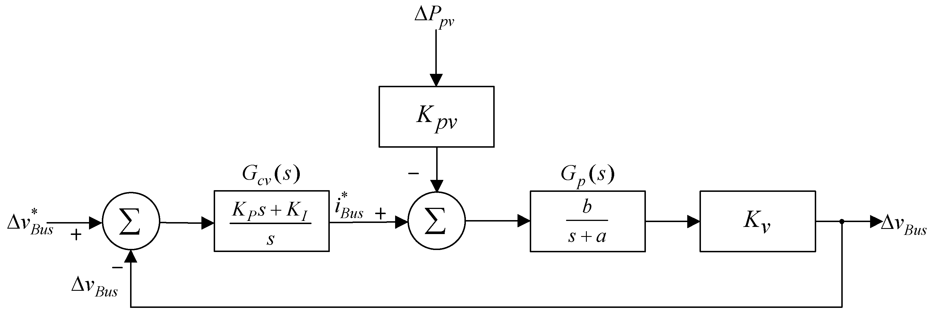
When carrying out estimation mode, the proportional controller is adopted as the voltage controller, making G_cv(s) = K_P = 10, then selecting an operating point (V_Bus = 180 V, P = 300 W), setting this system operation as closed-loop control. This paper hypothesizes that the dynamic model of the bidirectional buck–boost converter can be derived using the step response estimation method. Therefore, the parameter K_P of the proportional controller is given at will as long as the step response is without overshoot.

(b)

Given a step command ($\Delta v_{\mathrm{Bus}}^{*}=0.6$, K_v = 0.01, voltage V_Bus at high-voltage side increases from 180 V→240 V), then the measured variable waveform for the DC-link V_Bus voltage is shown in Figure 9; its steady-state voltage is at 220 V. The step command change Δv^*_Bus is also given arbitrarily, and K_v is the conversion factor of the voltage sensor.

(c)

Under the same operating conditions, given a set sunlight variation, so the output power variation is $\Delta {\mathrm{P}}_{\mathrm{p}v}=100\mathrm{W}$, which is P_pv from 1000 W→900 W, the measured DC-link voltage V_Bus variable waveform is shown in Figure 10, and the steady-state voltage is at 173 V.

(d)

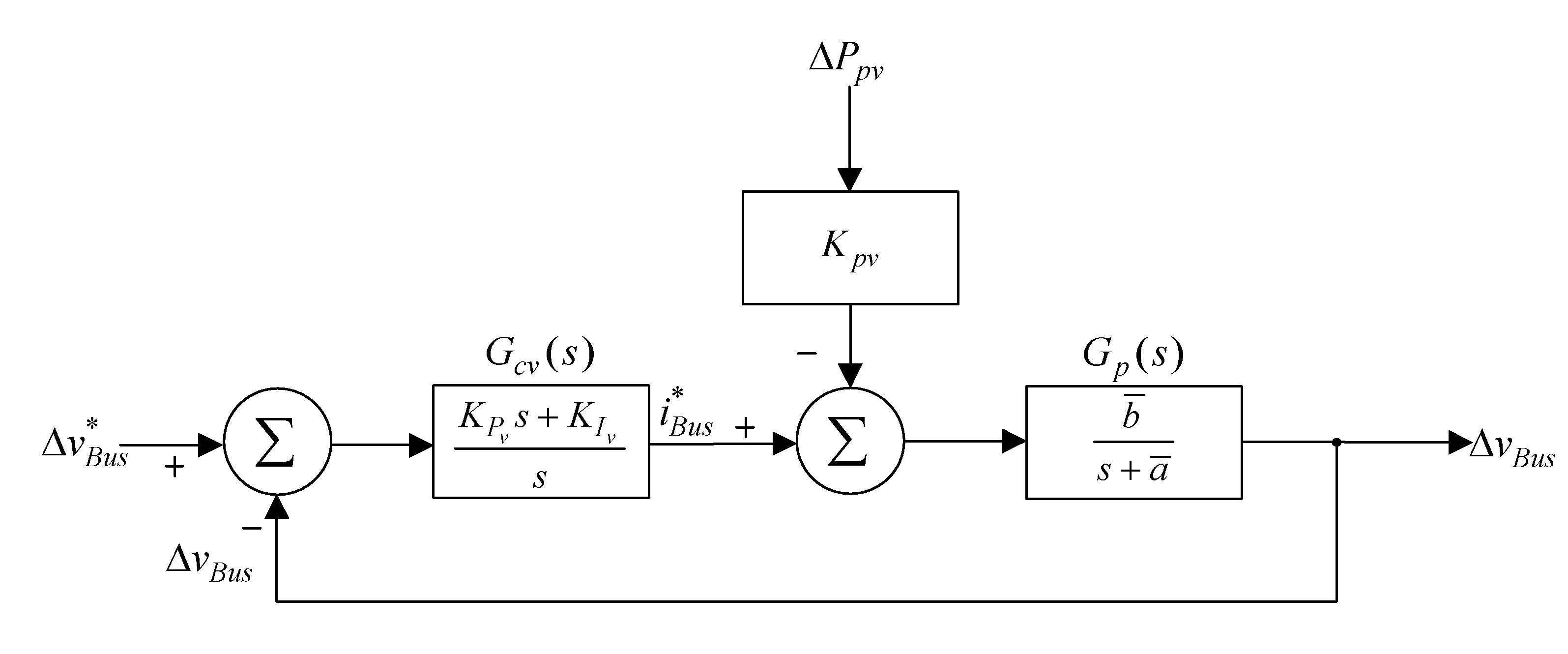
The transfer functions for $\Delta v_{\mathit{Bus}}^{}$ to $\Delta v_{\mathit{Bus}}^{*}$ and $\Delta v_{\mathit{Bus}}^{}$ to $\Delta P_{\mathit{pv}}$ can be derived from Figure 8 as shown in Equations (17) and (18), respectively.

$$H_v(s)=\frac{\Delta v_{Bus}}{\Delta v_{Bus}^{*}}\left|\begin{array}{l}\\ {}_{\Delta P_{pv}=0}\end{array}\right.=\frac{b{G}_{cv}{K}_v}{s+a+b{G}_{cv}{K}_v}\stackrel{\Delta }{=}\frac{c_1}{s+r}$$

(17)

$$H_p(s)=\frac{\Delta v_{Bus}}{\Delta P_{pv}}\left|\begin{array}{l}\\ {}_{\Delta v_{{}_{Bus}}^{*}=0}\end{array}\right.=\frac{-b{K}_{pv}{K}_v}{s+a+b{G}_{cv}{K}_v}\stackrel{\Delta }{=}-\frac{c_2}{s+r}$$

(18)

(e)

From the DC-link voltage step response shown in Figure 9, the steady-state value and the time to reach $(1-e^{-1})$ times the steady-state value can be observed and the parameters can be calculated as $c_1$ = 53.77 and r = 80.65.

(f)

The steady-state response of power step change can be obtained against DC-link voltage from Figure 10 and calculate $c_2$ = 0.056 and K_pv = 0.00967 from Equation (18).

(g)

a = 26.88 and b = 537.7 can be estimated from Equation (17); therefore, the transfer function G_p(s) of the bidirectional soft-switching converter can be written as:

$$G_p(s)=\frac{b}{s+a}=\frac{537.7}{s+26.88}$$

(19)

4.3. Quantitative Design of the Voltage Controller

The control block diagram in Figure 8 can be redrawn into Figure 11, the block diagram for the voltage control loop using P-I controller, where $\overline{a}=a=26.88$ and $\overline{b}=K_{v}b=5.377$, are the parameters for estimating the dynamic mode of the converter, while the DC-link voltage controller G_cv(s) adopts the P-I controller shown in Equation (20). The two parameters $K_{P_v}$ and K_Pv in Figure 11 are the conversion factor between the power and voltage and the proportional parameter of the P-I controller for the DC link voltage, respectively. Therefore, these two parameters not only have different symbols, but also have different meaning.

$$G_{cv}(s)=\frac{K_{P_v}s+K_{I_v}}{s}.$$

(20)

From Figure 11 control block diagram, the transfer function of $\Delta v_{Bus}$ to $\Delta P_{pv}$ is written as:

$$H_p(s)=\frac{\Delta v_{Bus}}{\Delta P_{pv}}\left|\begin{array}{l}\\ {}_{\Delta v_{Bus}^{*}=0}\end{array}\right.=\frac{-s{K}_{pv}\overline{b}}{s^2+\left(\overline{a}+\overline{b}{K}_P\right)s+\overline{b}{K}_I}\stackrel{\Delta }{=}\frac{-s{K}_{pv}\overline{b}}{\left(s+u_1\right)\left(s+u_2\right)}$$

(21)

Then, its unit step response can be presented as:

$$\Delta v_H(s)=\frac{H_P(s)}{s}=\frac{-K_{pv}\overline{b}\Delta P_{pv}}{s^2+\left(\overline{a}+\overline{b}{K}_P\right)s+\overline{b}{K}_I}\stackrel{\Delta }{=}\frac{-K_{pv}\overline{b}\Delta P_{pv}}{\left(s+u_1\right)\left(s+u_2\right)}$$

(22)

If the maximum value of this system transfer function can be designed into negative real root [27], the Equation (22) can be presented as:

$$\Delta v_H(s)=\frac{h_1}{s+u_1}+\frac{h_2}{s+u_2}$$

(23)

where:

$$\begin{array}{l}{u}_1+u_2=\overline{a}+\overline{b}{K}_P\\ u_1{u}_2=\overline{b}{K}_I\end{array}$$

(24)

$$h_1=-h_2=\frac{-K_{pv}\overline{b}\Delta P_{pv}}{u_1-u_2}$$

(25)

From Equations (22), (23) and (25), the unit step response can be re-written as:

$$\Delta v_H(t)=h_1{e}^{-u_{1}t}+h_2{e}^{-u_{2}t}=\frac{-K_{pv}\overline{b}\Delta P_{pv}}{u_1-u_2}(e^{-u_{1}t}+e^{-u_{2}t})$$

(26)

Then, differentiate the unit step response with respect to time, make $\Delta v_H(t)$ equal to 0 and find its extremum ${\widehat{v}}_{Bus,max}$ to obtain the maximum voltage drop ${\widehat{v}}_{Bus,max}$ and recovery time $t_{r,max}$, respectively, as:

$${\widehat{v}}_{Bus,max}=\frac{-K_{pv}\overline{b}\Delta P_{pv}}{u_1-u_2}\left[e^{\frac{-u_1}{u_1-u_2}\ln (\frac{u_1}{u_2})}-e^{\frac{-u_2}{u_1-u_2}\ln (\frac{u_1}{u_2})}\right]$$

(27)

$$t_{r,max}=\frac{1}{u_1-u_2}\ln (\frac{u_1}{u_2})$$

(28)

To allow the step response of the system to be equipped with characteristics of non-overshoot, zero steady-state error, quick voltage recovery time and minimized maximum voltage drop, once the specifications for maximum voltage drop and recovery time have been chosen, the two nonlinear equations can then be derived using Equations (27) and (28) as:

$$f_1(u_1,u_2)={\widehat{v}}_{Bus,\mathit{max}}-\frac{K_{pv}\overline{b}\Delta P_{pv}}{u_1-u_2}\left[e^{\frac{-u_1}{u_1-u_2}\ln \left(\frac{u_1}{u_2}\right)}-e^{\frac{-u_2}{u_1-u_2}\ln \left(\frac{u_1}{u_2}\right)}\right]$$

(29)

$$f_2(u_1,u_2)=0.05{\widehat{v}}_{Bus,\mathit{max}}-\frac{K_{pv}\overline{b}\Delta P_{pv}}{u_1-u_2}\left[e^{-u_1{t}_{r,max}}-e^{-u_2{t}_{r,max}}\right]$$

(30)

Calculate variables $u_1$ and $u_2$ for the two nonlinear equations using MATLAB software, and obtain $K_P$ and $K_I$ parameters for the voltage controller respectively based on Equation (24) as:

$$K_P^{}=\frac{\left(u_1+u_2\right)-\overline{a}}{\overline{b}}$$

(31)

$$K_I^{}=\frac{u_1{u}_2}{\overline{b}}$$

(32)

5. Test Results

Figure 12 and Figure 13 are the physical circuits and the experiment operating environment for the PVMA combined with the battery equalizing charge/discharge control developed for this paper, respectively. This paper used the programmable logic control DC power supply manufactured by Chroma Co., LTD (Taipei, Taiwan) to simulate the output of the PVMA, and by monitoring the positions of the operating points with the computer, we can confirm whether they can operate at the maximum power point. Moreover, since the power supply NGM202 [28] produced by the German Rohde & Schwarz Co. can simulate the charge status of the battery, to shorten the battery preset status during the experiment, this paper used the NGM202 in place of real batteries to carry out the actual test and used two sets of batteries with different voltages combined with the PVMA and MPPT technology to carry out the equalizing charge/discharge control experiment.

5.1. Response Performance Comparison between Quantitative Design and Traditional P-I Controller

Normal P-I controllers use the trial-and-error method to adjust the parameters of the controller; the control parameters under chosen operating points are obtained through continuous trials, and the maximum voltage drop ${\widehat{v}}_{Bus,max}$ and recovery time t_r that occur due to step variation cannot be regulated. Thus, this paper has designed controllers that meet the selected specifications via the quantitative method.

The transfer function of the bidirectional buck–boost soft-switching converter that is adopted in this paper is derived from Section 4.2 as shown in Equation (33), and the actual test on the controller is carried out under selected operating points (DC-link voltage V_Bus = 240 V and load P = 300 W).

$$G_p(s)=\frac{K_{v}b}{s+a}=\frac{\overline{b}}{s+\overline{a}}=\frac{5.377}{s+26.88}$$

(33)

The performance specifications set for the controller are as follows:

(1)

Non-overshoot.

(2)

No steady-state error.

(3)

From the maximum voltage drop ${\widehat{v}}_{Bus,max}=0.1\mathrm{V}/\mathrm{W}$ induced by the step sunlight variation (that is, photovoltaic module array output power variation) (meaning $100\mathrm{W}\to 10\mathrm{V}$ ).

(4)

From the voltage recovery time induced by the step sunlight variation $t_r=0.5s$.

From Equations (29) to (32), the respective voltage control parameters of the quantitative design are obtained as:

$$K_{Pv}=0.25\hspace{1em}{K}_I{}_v=4.81$$

(34)

To validate the feasibility of the quantitatively designed controller, the DC-link voltage control response waveform of both the quantitatively designed controller and the traditional P-I controller ($K_{Pv}=0.1$,$K_I{}_v=1.2$) obtained from the trial-and-error method is tested under the same conditions. Figure 12 is the DC-link voltage response waveform of the quantitatively designed controller under sunlight variation; it can be observed from the Figure 14 that regardless of how sunlight changes, the voltage response all meet the above-defined specifications, whereas Figure 15 is the voltage response waveform of the traditional P-I controller by the trial-and-error method. It can be observed from Figure 15 that there is little difference in the voltage variation range compared to the quantitatively designed controller, yet the recovery time is increased by 0.3 s.

As per the measured results, the parameters established for the DC-link voltage PI controller of the bidirectional buck–boost converter are illustrated in Figure 14a, as designed by the quantitative method. In the meantime, the insolation is shown in DC-link voltage waveform measured when 1000 W/m² drops to 900 W/m². From the figure, we see that lowering the insolation resulted in lowering the output power for the photovoltaic module array to incur the sudden dropping of DC-link voltage. Because the PI controller parameters are designed by the quantitative method according to the preset performance specifications (including the maximum voltage drop of DC-link voltage and its recovery time), DC-link voltage is restored to the set 240 V for about 0.5 s. Indicated in Figure 15a is the waveform measured by the conventional PI controller under the same conditions and its recovery time will be 0.8 s. As such, there is a 0.3 s difference in response speed between both of them. Likewise, when the insolation rises to 1000 W/m² from 900 W/m², the DC-link voltage suddenly increases due to the output power in the photovoltaic module array. In Figure 14b, we see that the quantitative PI controller allows the DC-link voltage to restore the set 240 V in about 0.5 s. Shown in Figure 15b is the waveform measured by the conventional PI controller under the same conditions and its restoration time is about 0.8 s. Same as above, there is a 0.3 s difference in the response speed between both of them. If the PI controller parameters are designed by a quantitative method according to the preset performance specifications, it allows the DC-link voltage to restore to the set 240 V more quickly under the specified maximum voltage drop.

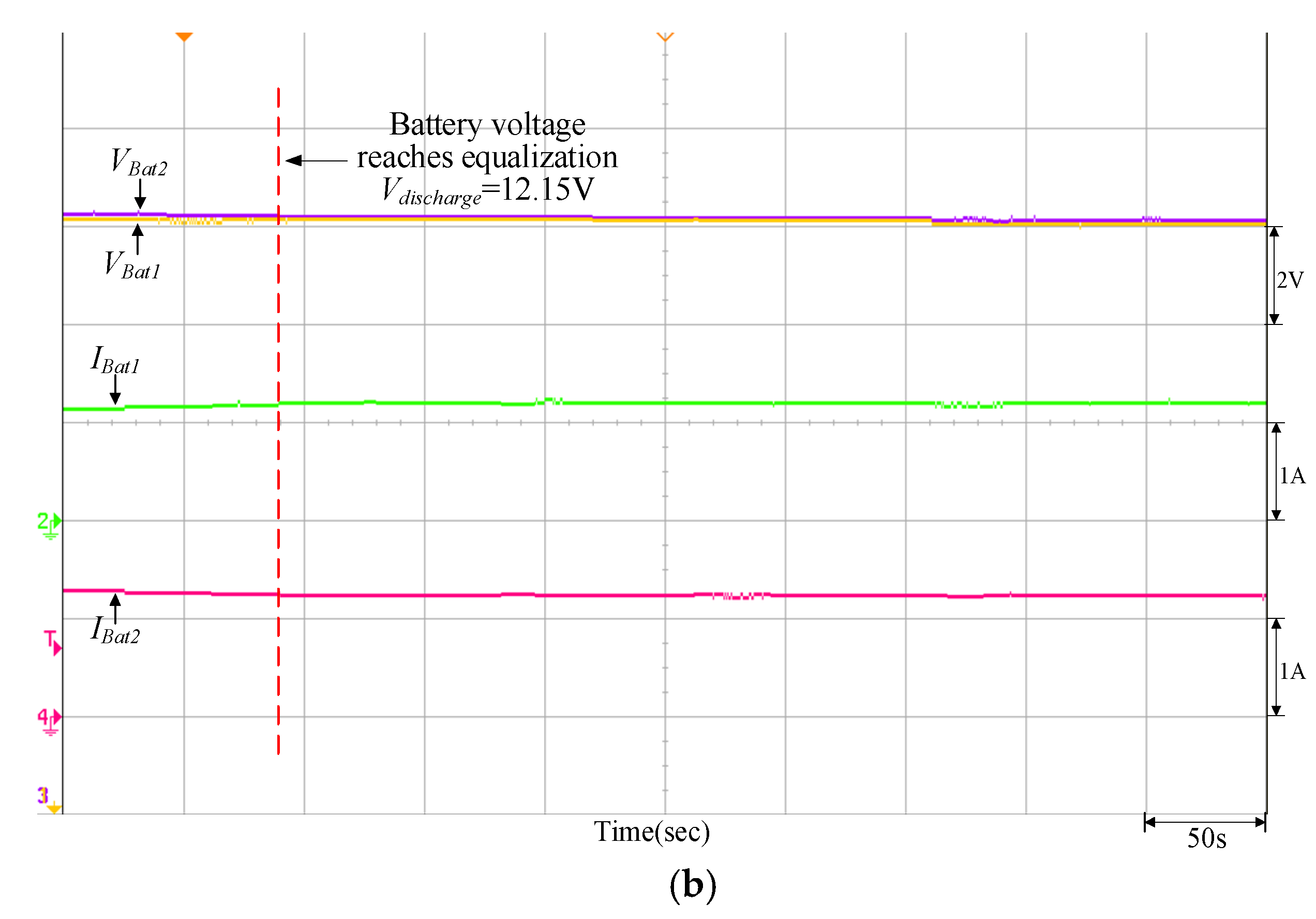
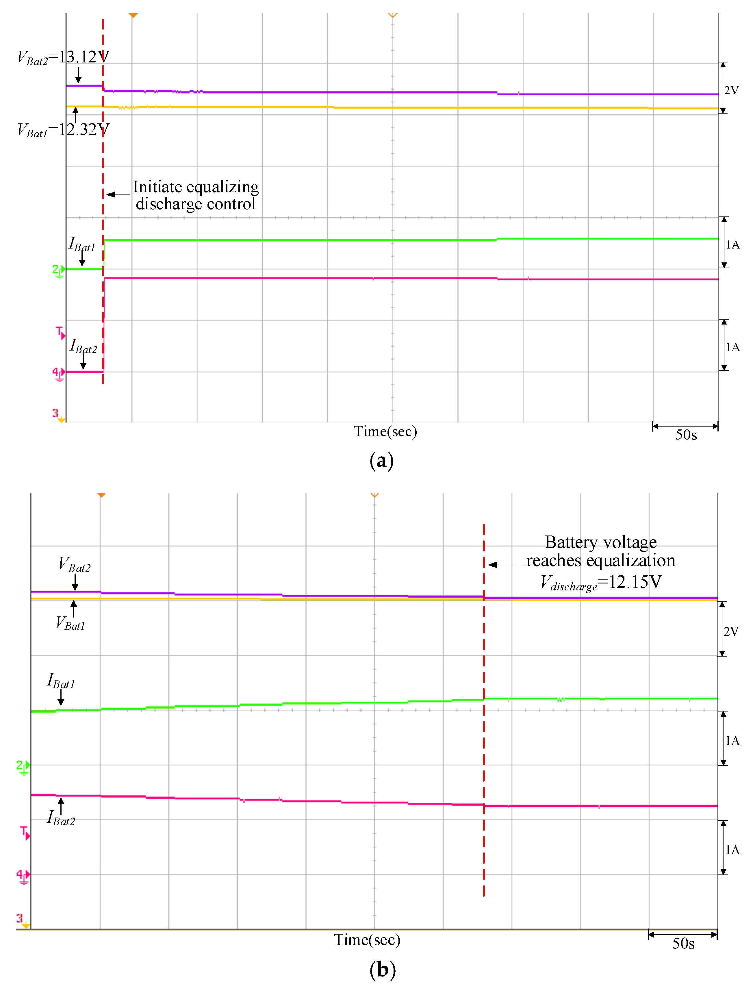
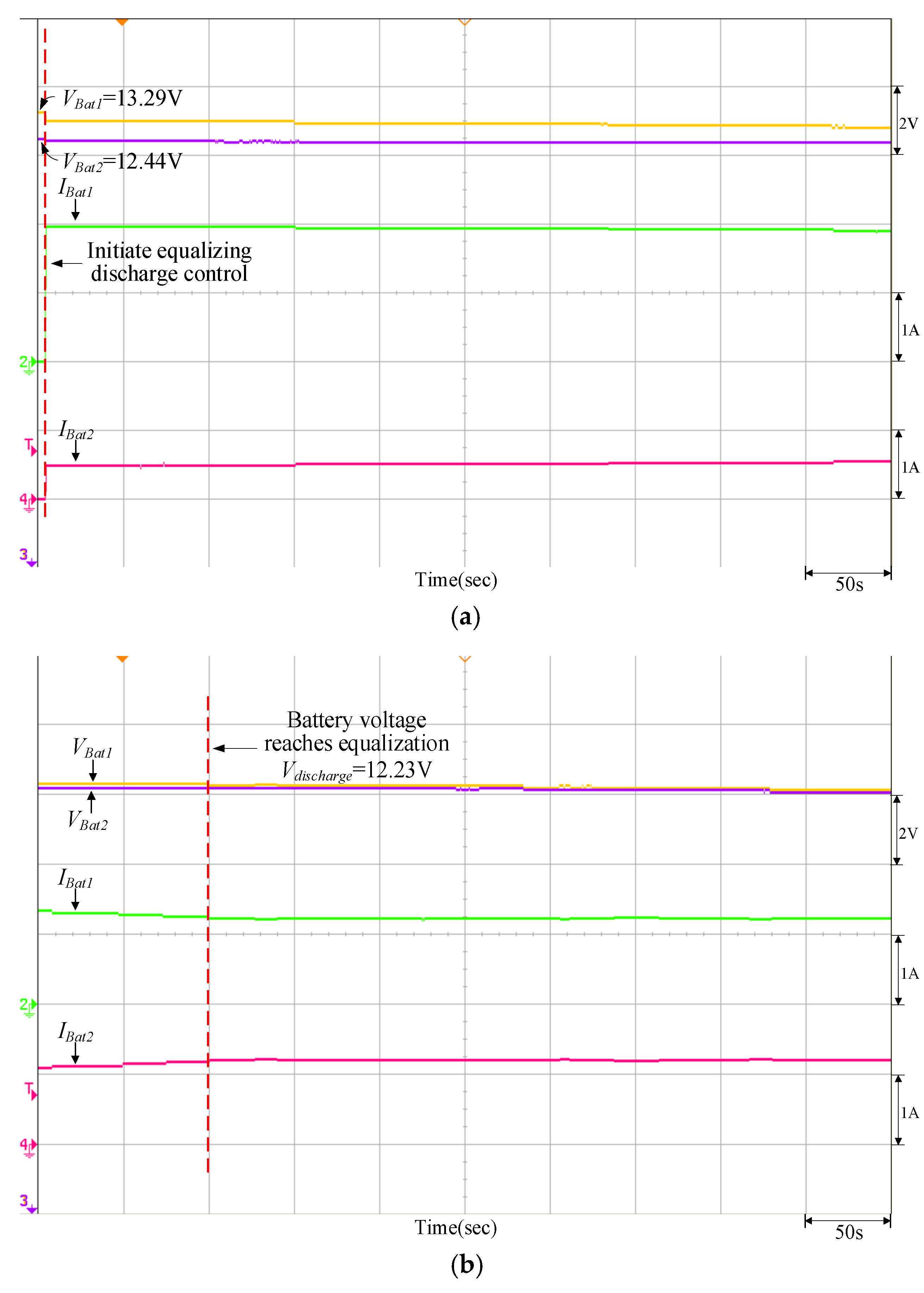
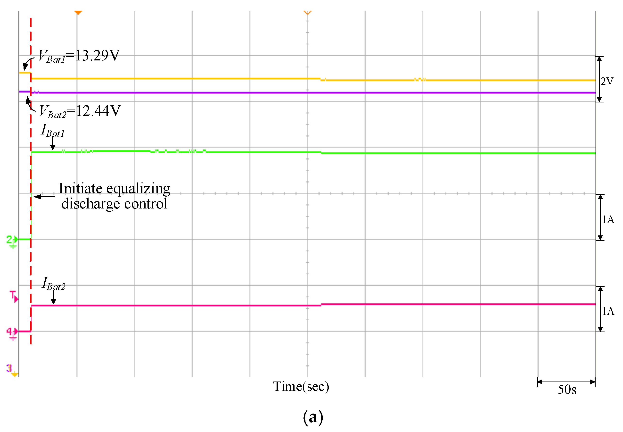
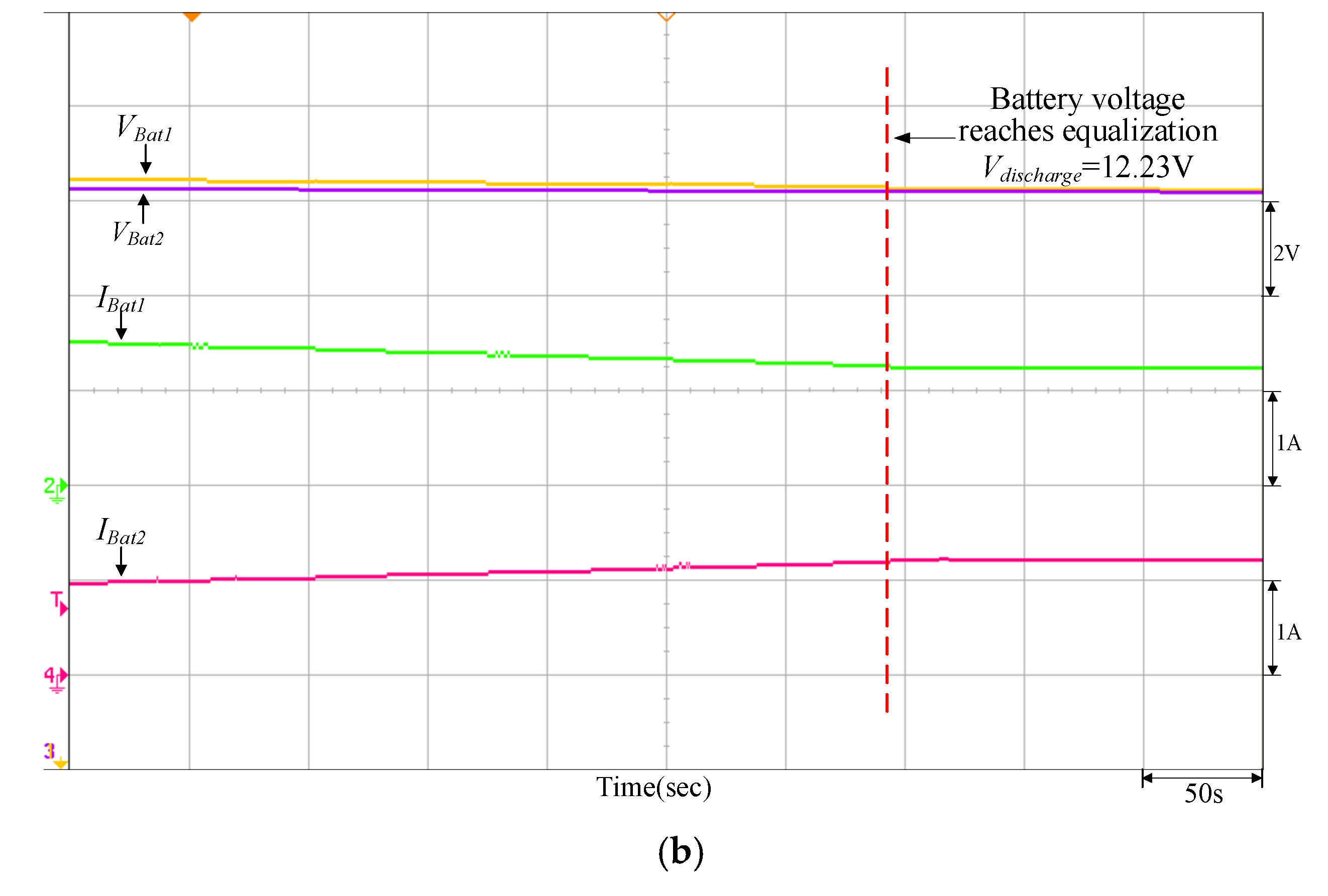
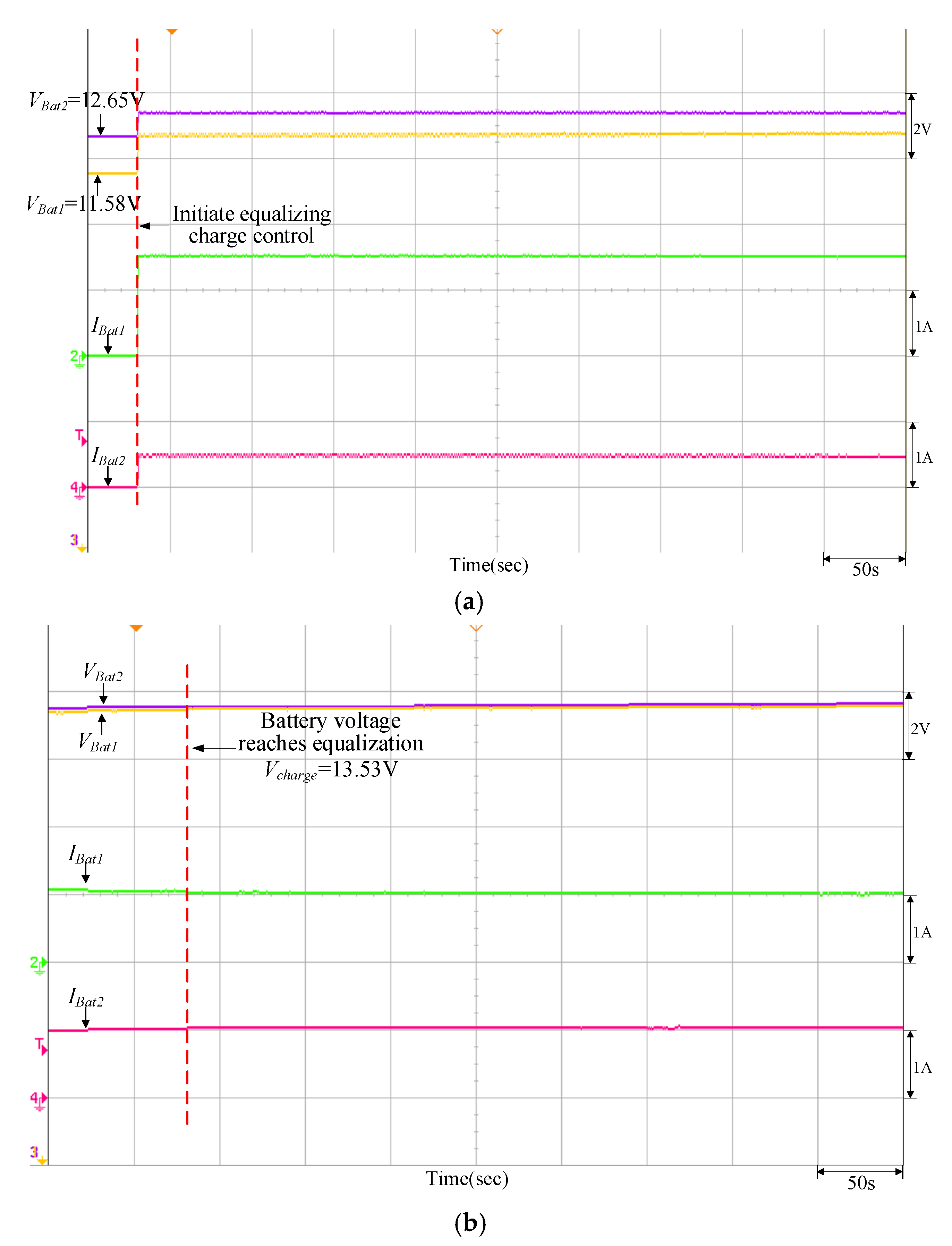
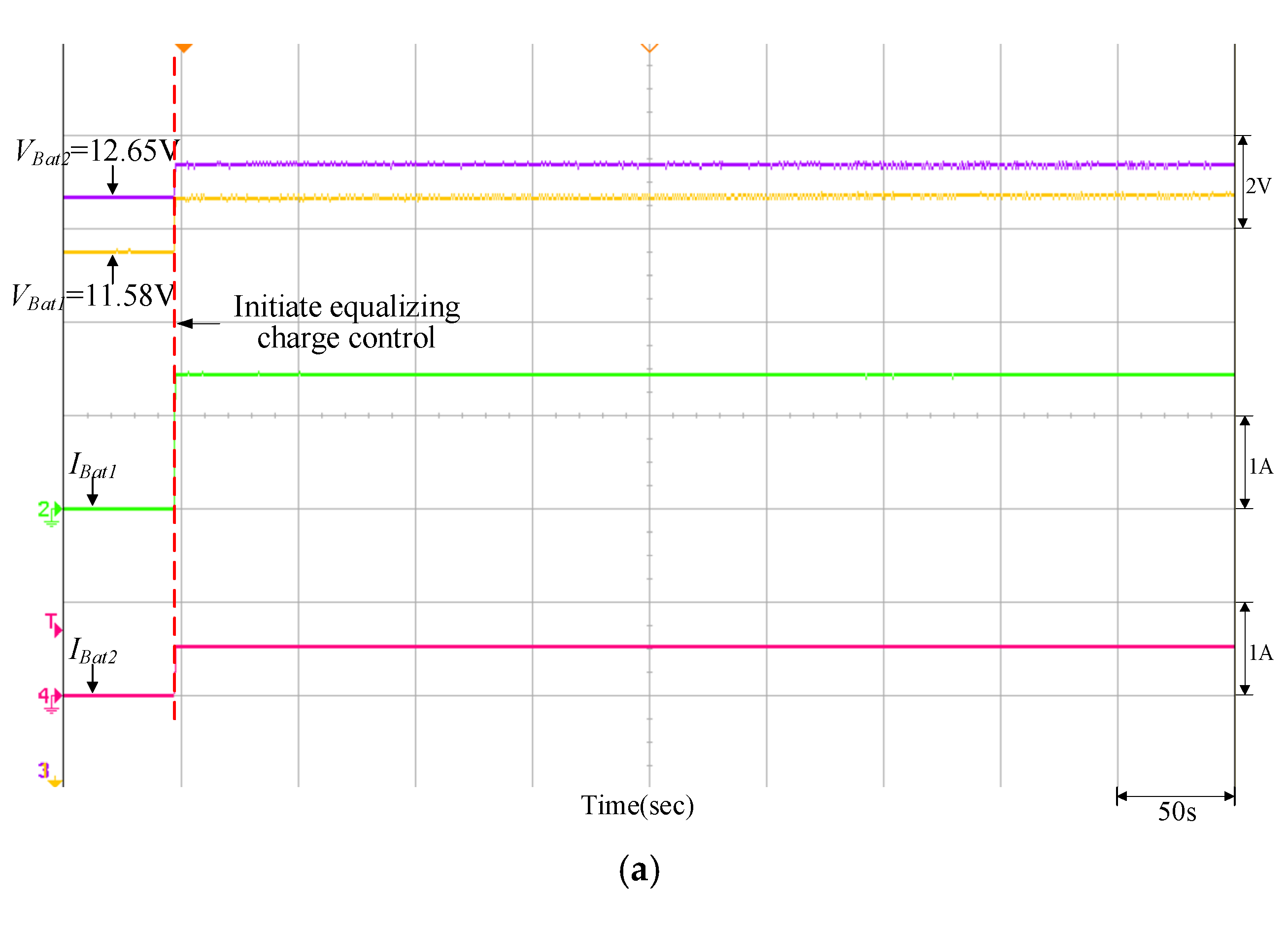
5.2. Response Test for the Photovoltaic Array Combined with the Equalizing Charge/Discharge Controller

The soft-switching bidirectional buck–boost converter adopted in this paper is applied to two sets of batteries with different voltages, while both are combined with the PVMA and the MPPT technology to carry out the actual testing of equalizing charge/discharge control. Then, a comparison is made between the response speed and performance for the charge/discharge of the adopted quantitatively designed controller and the traditional P-I controller to validate the feasibility of the adopted controller and system architecture. The power supply NGM202 is used to simulate the 12 V/5 Ah lead-acid battery during the actual test; however, since the time for the oscilloscope to record the waveform during the battery equalizing charge/discharge control response process is quite long, the following measured control process response can only show the initiation of the equalizing charge/discharge control and the process to reach equalization.

Table 3. Initial voltage and final voltage after reaching equalizing charge/discharge of each battery set under different PVMA output power.

Operating Mode	Voltage Status
	Initial Voltage of First Set	Final Equalizing Charge/Discharge Voltage	Initial Voltage of Second Set	Final Equalizing Charge/Discharge Voltage
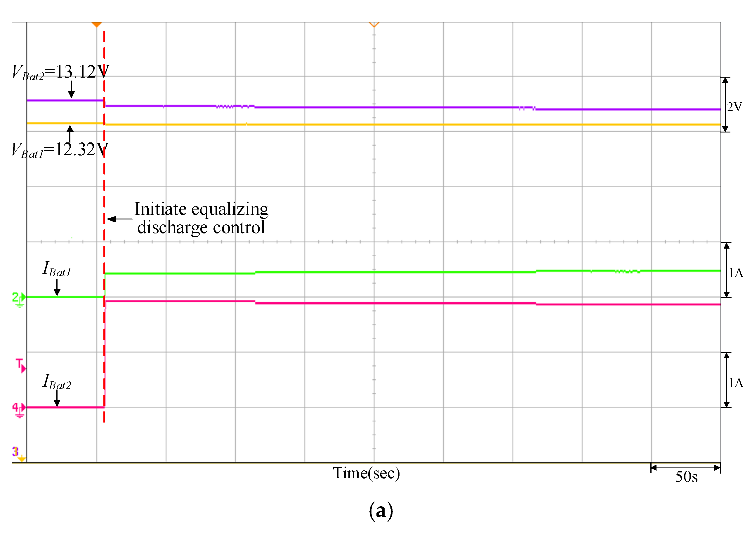
Discharging	VBat1 = 12.32 V	Vdischarge = 12.15 V (PV power = 200 W)	VBat1 = 13.29 V	Vdischarge = 12.23 V (PV power = 200 W)
	VBat2 = 13.12 V		VBat2 = 12.44 V
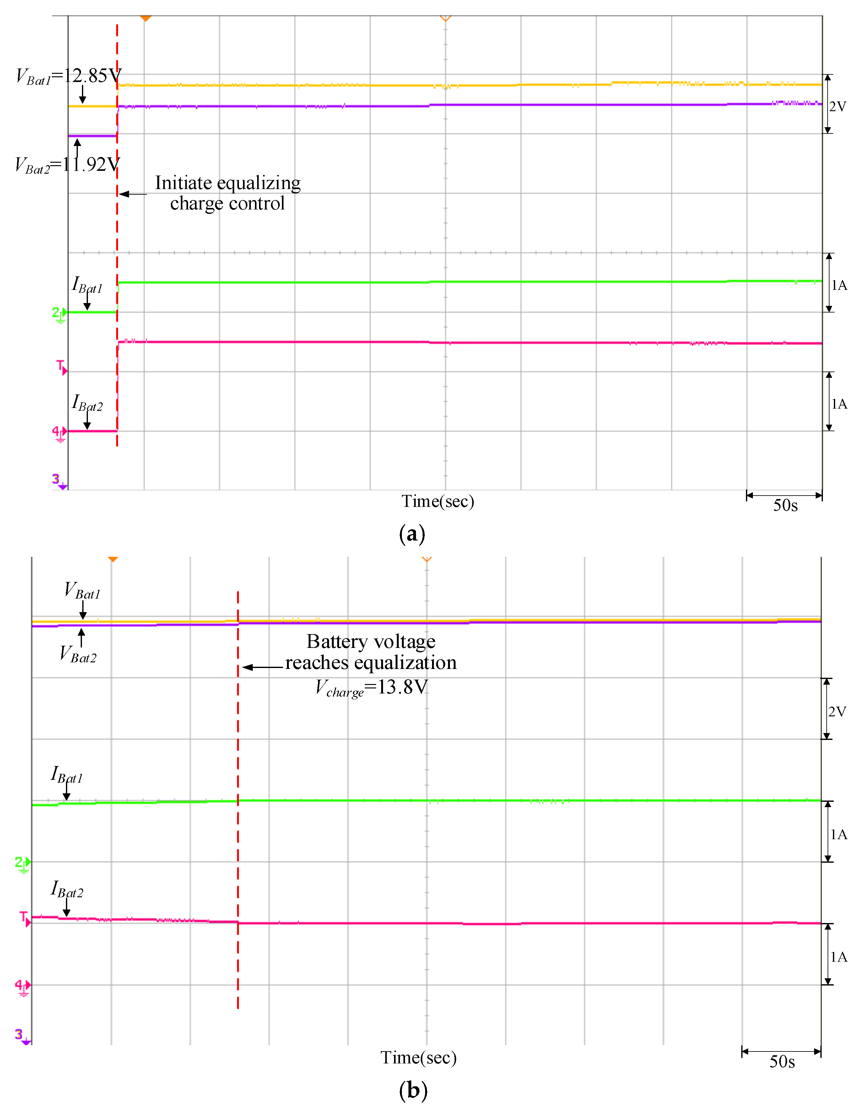
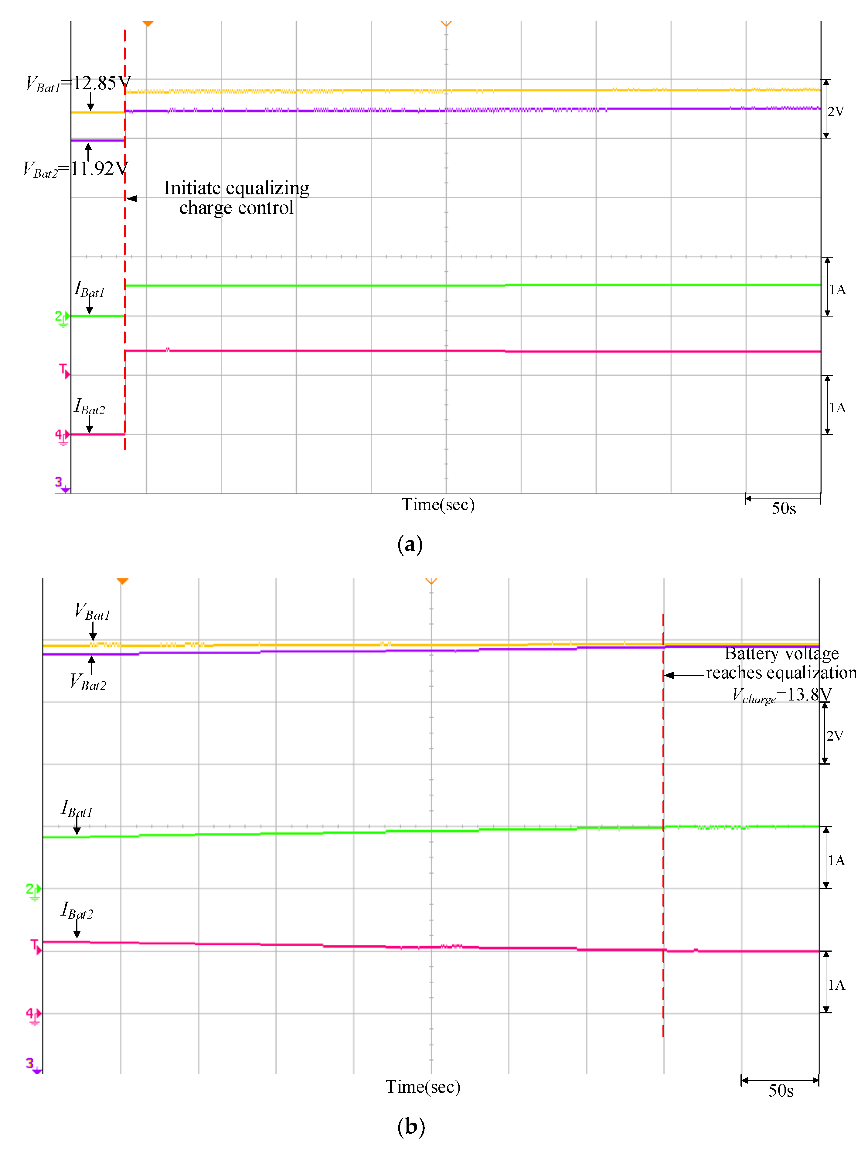
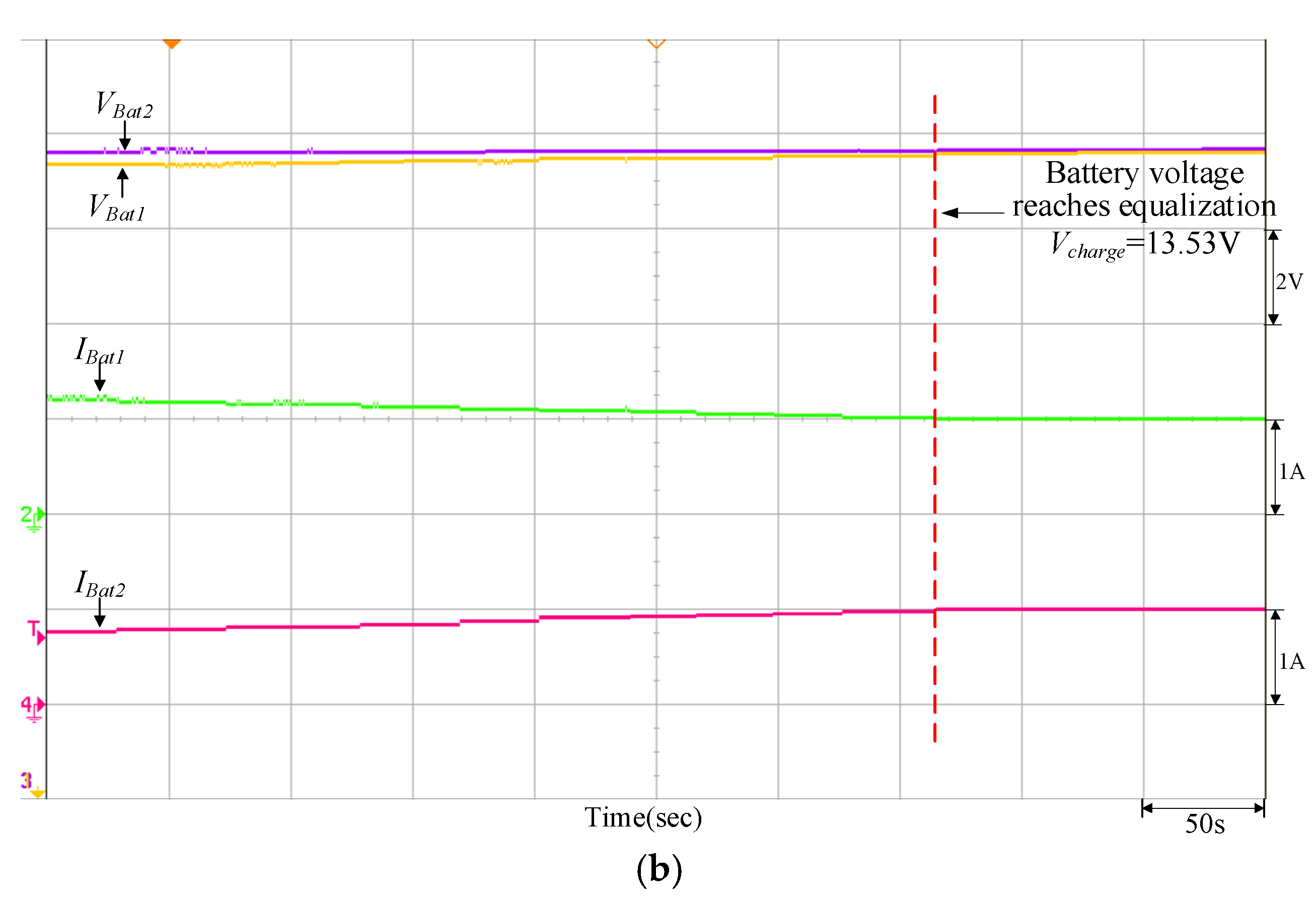
Charging	VBat1 = 11.58 V	Vcharge = 13.53 V (PV power = 400 W)	VBat1 = 12.85 V	Vcharge = 13.8 V (PV power = 400 W)
	VBat2 = 12.65 V		VBat2 = 11.92 V

lists the initial voltage and final voltage after reaching equalizing charge/discharge of each battery set under different PVMA output power.

Figure 16 is the P-V characteristic curve of the PMVA when the maximum power point is at 200 W. Figure 17, Figure 18, Figure 19 and Figure 20 are measured waveforms of the battery under equalizing discharge control on the load end when the PVMA output power is at 200 W. At this time, the current of the bidirectional buck–boost soft-switching converter flows from the battery end of the low-voltage side to the load end of the high-voltage side; thus, the accumulator battery current is positive. Among them, Figure 17 and Figure 19 are the equalizing discharge response waveforms of the adopted quantitatively designed controller, and Figure 18 and Figure 20 are the equalizing discharge response waveforms of the traditional P-I controller. By comparing Figure 17, Figure 18, Figure 19 and Figure 20, it can be observed that the equalizing discharge speed response of the adopted quantitatively designed controller is better than the traditional P-I controller, and the time required to reach equalization for both is compiled in

Table 4. Comparison of equalizing discharge time between the quantitatively designed controller and traditional P-I controller.

Controller Used	Battery Status
	VBat1 = 12.32 V VBat2 = 13.12 V	VBat1 = 13.29 V VBat2 = 12.44 V
Quantitatively designed controller	33 m 54 s	34 m 55 s
Traditional P-I controller	38 m 28 s	39 m 05 s

.

Figure 21 is the P-V characteristic curve of the PMVA when the maximum power point is at 400 W. Figure 22, Figure 23, Figure 24 and Figure 25 are measured waveforms of the battery under equalizing charge control on the load end when the PVMA output power is at 400 W. At this time, the current of the bidirectional buck–boost soft-switching converter flows from the load end of the high-voltage side to the battery end of the low-voltage side; thus, the accumulator battery current is negative; to protect the battery from damage, the maximum charging current is set to 0.3 C. Among them, Figure 22 and Figure 24 are the equalizing charge response waveforms of the adopted quantitatively designed controller, and Figure 23 and Figure 25 are the equalizing charge response waveforms of the traditional P-I controller. From Figure 22, Figure 23, Figure 24 and Figure 25, it can be observed that the equalizing charge speed response of the adopted quantitatively designed controller is better than the traditional P-I controller, and the time required to reach equalization for both is compiled in

Table 5. Comparison of equalizing charge time between the quantitatively designed controller and traditional P-I controller.

Controller Used	Battery Status
	VBat1 = 11.58 V VBat2 = 12.65 V	VBat1 = 12.85 V VBat2 = 11.92 V
Quantitatively designed controller	42 m 31 s	41 m 40 s
Traditional P-I controller	46 m 40 s	46 m 04 s

.

It can be observed from Figure 16, Figure 17, Figure 18, Figure 19 and Figure 20 that when the PVMA output power (P_pv) is lower than the load power, the battery will discharge as an auxiliary power supply; conversely, it can be observed from Figure 21, Figure 22, Figure 23, Figure 24 and Figure 25 that if the PVMA output power (P_pv) is higher than the load power, the battery will charge to keep the DC-link voltage (V_Bus) constant. The greater the voltage difference between the two batteries, the time required for charge/discharge will be comparatively longer, and the discharging current for the battery with more energy storage is greater during the initial discharge; on the other hand, during the initial charge, the charging current for the battery with more energy storage is smaller.

It can be observed from Figure 17, Figure 18, Figure 19 and Figure 20 and Figure 22, Figure 23, Figure 24 and Figure 25 that when the equalizing charge/discharge control is completed, the voltage in the two batteries will be the same, and the charge/discharge current will also be the same, thus achieving the goal of equalizing charge/discharge. Actual test results have proven that the parameters of the P-I controller will affect the battery equalizing charge/discharge speed; therefore, to meet the expected charge/discharge response, the controller needs to be designed. It can be seen from Table 4 and Table 5 that the equalizing charge/discharge time of the adopted quantitatively designed controller is shortened by more than 10% as compared to the traditional P-I controller. Furthermore, as the battery charge/discharge rate will affect the battery equalizing charge/discharge time, if the restriction on maximum current from original settings remains unchanged, the charge/discharge time will become longer when batteries with larger capacity are used.

The photovoltaic module can convert light energy to electric energy. When affected by the insolation and the environment temperature, it will cause the fluctuation of the output P-V characteristic curve. When the insolation increases or reduces, the photovoltaic module’s output power will change. When the insolation is increased or reduced, its output current will present a more significant increasing or reducing amplitude; however, less increasing/reducing amplitude is observed for the output voltage. Although the output power will change along with the temperature fluctuation of the photovoltaic module, it is different from the change incurred by the insolation. This is because when the temperature changes, the output current presents less prominent amplitude variation; instead, more signification variation is observed in the output voltage amplitude. Figure 16 and Figure 21 illustrate the P-V output characteristic curve of the photovoltaic module array simulator when measured under the same temperature range. Due to varied insolation, I_sc and I_mp present more prominent amplitude change but that of V_oc and V_mp is not so prominent.

The waveform that has been recorded by the oscilloscope during the battery equalizing charge/discharge control response process is used in this paper. Because its charging/discharging process is very long, to avoid occupying too much space, the initial stage, when the equalizing charge/discharge control is activated and the final stage, when achieving the equalization is illustrated in the response waveform as being drafted for the entire control process. However, the total time required to reach a steady state for both the equalizing charges/discharges of different cases are list in Table 4 and Table 5, respectively.

The photovoltaic module array can convert the light energy to electric energy to supply the required load. As soon as the insolation increases, the output power of the photovoltaic module array will increase. If the generated electricity exceeds the level required for the load, it will transfer the excessive energy to the battery through the bidirectional buck–boost converter and then the charged power will be stored in the battery. If the generated electricity is insufficient to supply the load end, the storage battery will supply the backup power to the load end through the bidirectional buck–boost converter as well.

To achieve faster charging and discharging speed for the battery, we conducted the quantitative design for the controller of the bidirectional buck–boost converter. First, the transfer function is induced for the bidirectional buck–boost converter according to the estimated step response result and then the quantitative design is conducted for the control parameters according to the selected control performance specifications. In the meantime, two sets of batteries designed with different voltage ratings are used to compare the equalizing charging and discharging speed response between the quantitative-based PI controller and the conventional PI controller. The measured result supports that the equalizing charge/discharge time of the quantitative-based controller is shorter than the conventional PI controller by 10% and so it can achieve the intended equalizing charge/discharge control effect for the battery. When the operation point of the converter changes, the quantitative-based PI controller can also achieve satisfactory DC-link voltage control performance. In addition, the battery equalizing charge/discharge control architecture mentioned in Reference [17] is used in this paper. However, the parameters of the charge/discharge PI controller mentioned in Reference [17] are acquired through the “trial and error” method; therefore, a longer amount of time will be required in order to obtain appropriate controller parameters. Compared to the “trial and error” method, the controller parameters can be obtained faster through the quantitative design executed for the PI controller parameters at the operation point selected for the converter being used in this paper. In the meantime, it also allows the converter to achieve the intended control performance.

Because each battery cell is provided with a suitable charging/discharging rate, so the charging/discharging current is limited to 0.3 C so as to avoid creating excessive current as to cause battery damage when charging/discharging the lead-acid battery. Because the voltage and the capacity of both battery cells are different during the initial charge, so lower-power battery is charged with a higher current, whereas the higher-power battery is charged with a lower current. When both battery cells are gradually equalizing, the charging current of both battery cells will become nearly equalized. Finally, equalized electric energy is achieved for each of the battery cells. On the other hand, because the voltage and the capacity of both battery cells are different during the initial discharge, so lower-power battery is discharged with a lower current, whereas the higher-power battery is discharged with a higher current. When both battery cells are gradually equalizing, the discharging current of both battery cells will become nearly equalized. Finally, equalized electric energy is achieved for each of the battery cells. Therefore, the bigger the difference in battery power, the longer the battery equalizing time; on the contrary, the smaller the difference in battery power, the shorter the battery equalizing time.

6. Conclusions

This paper uses the PVMA combined with the energy storage system architecture of the battery equalizing charge/discharge control as the topic of study. The tilt angle of the photovoltaic module creates less influence when compared with that incurred by the insolation to the power generation capacity. Because the maximum power point tracking (MPPT) method is selected for the photovoltaic module array in this paper, it allows it to output the maximum power under varied insolation conditions. First, the adopted bidirectional buck–boost soft-switching converter is developed, then two sets of converters are serial-connected to construct an equalizing charge/discharge architecture, and the digital signal processor TMS320F2809 is used as the control core together with the PVMA and the MPPT technology. Then, by following the planned battery charge/discharge control strategy, the battery set can achieve equalizing charge/discharge. To increase the speed of battery charge/discharge, the controller for the bidirectional converter undergoes quantitative design. First, the result is estimated through step response where the transfer function of the bidirectional converter is derived, then by following the defined control performance, the controller undergoes quantitative design. Then, comparisons on the equalizing charge/discharge speed response are made between the new design and the traditional P-I controller using two sets of batteries with different voltages. From the test results, it has been proven that the equalizing charge/discharge time of the adopted quantitatively designed controller is shortened by 10% compared to the traditional P-I controller, and the battery equalizing charge/discharge control effects can indeed be achieved.

References

- Botelho, A.; Pinto, L.M.C.; Louren-Gomes, L.; Valente, M.; Social, S. Sustainability of Renewable Energy Sources in Electricity Production: An Application of the Contingent Valuation Method. Sustain. Cities Societ. 2016, 26, 429–437. [Google Scholar] [CrossRef]
- Okonkwo, P.C.; Mansir, I.B.; Barhoumi, E.M.; Emori, W.; Radwan, A.B.; Shakoor, R.A.; Uzoma, P.C.; Pugalenthi, M.R. Utilization of Renewable Hybrid Energy for Refueling Station in Al-Kharj, Saudi Arabia. Int. J. Hhydr. Energy 2022, 47, 22273–22284. [Google Scholar] [CrossRef]
- Alhousni1, F.K.; Ismail1, F.B.; Okonkwo, P.C.; Mohamed, H.; Okonkwo, B.O.; Al-ShahriA, O.A. Review of PV Solar Energy System Operations and Applications in Dhofar Oman. AIMS Energy 2022, 10, 858–884. [Google Scholar] [CrossRef]
- Pérez-Deniciaa, E.; Fernández-Luqueñob, F.; Vilariño-Ayalac, D.; Montaño-Zetinad, L.M.; Maldonado-López, L.A. Renewable Energy Sources for Electricity Generation in Mexico: A Review. Renew. Sust. Energy Rev. 2017, 78, 597–613. [Google Scholar] [CrossRef]
- Beitelmal, W.H.; Okonkwo, P.C.; Housni, F.A.; Grami, S.; Emori, W.; Uzoma, P.C.; Das, B.K. Renewable Energy as a Source of Electricity for Murzuq Health Clinic during COVID-19. MRS Energy Sustain. 2022, 9, 79–93. [Google Scholar] [CrossRef]
- Chao, K.H.; Huang, B.Z.; Jian, J.J. An Energy Storage System Composed of Photovoltaic Arrays and Batteries with Uniform Charge/Discharge. Energies 2022, 15, 2883. [Google Scholar] [CrossRef]
- Ramireddy, K.; Hirpara, Y.; Kumar, Y.V.P. Transient performance analysis of buck boost converter using various PID gain tuning methods. In Proceedings of the 12th International Conference on Computational Intelligence and Communication Networks (CICN), Bhimtal, India, 25–26 September 2020; pp. 321–326. [Google Scholar]
- Lei, W.; Li, C.; Chen, M.Z.Q. Robust Adaptive Tracking Control for Quadrotors by Combining PI and Self-tuning Regulator. IEEE Trans. Control Syst. Technol. 2019, 27, 2663–2671. [Google Scholar] [CrossRef]
- Kaicheng, D.; Yan, Z.; Jinjun, L.; Pengxiang, Z.; Jinshui, Z. Dynamic performance improvement of bidirectional switched-capacitor DC/DC converter by right-half-plane zero elimination. In Proceedings of the International Power Electronics Conference (IPEC-Niigata 2018-ECCE Asia), Niigata, Japan, 20–24 May 2018; pp. 4181–4185. [Google Scholar]
- Kesarkar, A.A.; Narayanasamy, S. Asymptotic Magnitude Bode Plots of Fractional-order Transfer Functions. IEEE/CAA J. Autom. Sin. 2019, 6, 1019–1026. [Google Scholar] [CrossRef]
- Tufenkci, S.; Senol, B.; Alagoz, B.B. Disturbance rejection fractional order PID controller design in V-domain by particle swarm optimization. In Proceedings of the International Artificial Intelligence and Data Processing Symposium (IDAP), Malatya, Turkey, 21–22 September 2019; pp. 1–6. [Google Scholar]
- Nicola, M.; Nicola, C.I. Improved performance of grid-connected photovoltaic system based on fractional-order PI controller and particle swarm optimization. In Proceedings of the 9th International Conference on Modern Power Systems (MPS), Cluj-Napoca, Romania, 16–17 June 2021; pp. 1–5. [Google Scholar]
- Tufenkci, S.; Senol, B.; Alagoz, B.B. Stabilization of fractional order PID controllers for time-delay fractional order plants by using genetic algorithm. In Proceedings of the International Conference on Artificial Intelligence and Data Processing (IDAP), Malatya, Turkey, 28–30 September 2018; pp. 1–6. [Google Scholar]
- Peng, C.C.; Lee, C.L. Performance demands based servo motor speed control: A genetic algorithm proportional-integral control parameters design. In Proceedings of the International Symposium on Computer, Consumer and Control (IS3C), Taichung City, Taiwan, 13–16 November 2020; pp. 469–472. [Google Scholar]
- Wang, Y.; Ying, Z.; Zhang, W. Unified sliding mode control of boost converters with quantitative dynamic and static performances. In Proceedings of the 46th Annual Conference of the IEEE Industrial Electronics Society (IECON 2020), Singapore, 18–21 October 2020; pp. 3271–3276. [Google Scholar]
- Mohanty, S.; Choudhury, A.; Pati, S.; Kar, S.K.; Khatua, S. A comparative analysis between a single loop PI, double loop PI and sliding mode control structure for a buck converter. In Proceedings of the 1st Odisha International Conference on Electrical Power Engineering, Communication and Computing Technology (ODICON), Bhubaneswar, India, 8–9 January 2021; pp. 1–6. [Google Scholar]
- Li, Z.; Yuan, Y.; Wang, H.N. Fuzzy adaptive time-delay feedback controlling chaos in buck converter. In Proceedings of the Chinese Control and Decision Conference (CCDC), Hefei, China, 22–24 August 2020; pp. 4732–4737. [Google Scholar]
- Aarti, D.S.; Arun, N.K. Liquid level control of quadruple conical tank system using linear PI and fuzzy PI controllers. In Proceedings of the 2nd International Conference for Emerging Technology (INCET), Belagavi, India, 21–23 May 2021; pp. 1–5. [Google Scholar]
- Liu, Z.H.; Nie, J.; Wei, H.L.; Chen, L.; Li, X.H.; Lv, M.Y. Switched PI Control Based MRAS for Sensorless Control of PMSM Drives Using Fuzzy-logic-controller. IEEE J. Power Electron. 2022, 3, 368–381. [Google Scholar] [CrossRef]
- Naung, Y.; Anatolii, S.; Lin, Y.H. Speed control of DC motor by using neural network parameter tuner for PI-controller. In Proceedings of the IEEE Conference of Russian Young Researchers in Electrical and Electronic Engineering (EIConRus), Saint Petersburg and Moscow, Russia, 28–31 January 2019; pp. 2152–2156. [Google Scholar]
- Chao, K.H.; Huang, C.H. Bidirectional DC-DC Soft-switching Converter for Stand-alone Photovoltaic Power Generation Systems. IET Power Electron. 2014, 7, 1557–1565. [Google Scholar] [CrossRef]
- Jian, J.J. Energy Storage System with Uniform Battery Charging and Discharging Control. Master’s Thesis, National Chin-Yi University of Technology, Taichung City, Taiwan, 23 July 2020. [Google Scholar]
- Ram, J.P.; Pillai, D.S.; Rajasekar, N.; Strachan, S.M. Detection and Identification of Global Maximum Power Point Operation in Solar PV Applications Using a Hybrid ELPSO-P&O Tracking Technique. IEEE Trans. Emerg. Sel. Topics Power Electron. 2020, 8, 1361–1374. [Google Scholar]
- Tang, C.Y.; Wu, H.J.; Liao, C.Y.; Wu, H.H. An Optimal Frequency-modulated Hybrid MPPT Algorithm for the LLC Resonant Converter in PV Power Applications. IEEE Trans. Power Electron. 2022, 37, 944–954. [Google Scholar] [CrossRef]
- TMS320F2809 Data Manual, Texas Instruments. October 2003. Available online: https://www.ti.com/lit/ds/symlink/tms320f2809.pdf?ts=1594465026502&ref_url=https%253A%252F%252Fwww.ti.com%252Fprodu107ct%252FTMS320F2809.pdf (accessed on 23 August 2022).
- Gao, Z.H.; Xie, H.C.; Yang, X.B.; Niu, W.F.; Li, S.; Chen, S.Y. The Dilemma of C-Rate and Cycle Life for Lithium-Ion Batteries under Low Temperature Fast Charging. Batteries 2022, 8, 234. [Google Scholar] [CrossRef]
- Chen, P.Y.; Chao, K.H.; Chen, H.J. Modeling and Quantitative Design of a Controller for a Bidirectional Converter with High Voltage Conversion Ratio. Int. J. Innov. Comput. Inf. Control 2018, 14, 2203–2219. [Google Scholar]
- R&S®NGL200/NGM200 Power Supply Series User Manual. Available online: https://scdn.rohde-schwarz.com/ur/pws/dl_downloads/pdm/cl_manuals/user_manual/1178_8736_01/NGL200_NGM200_UserManual_en_10.pdf. (accessed on 23 August 2022).