Early Prediction of the Health Conditions for Battery Cathodes Assisted by the Fusion of Feature Signal Analysis and Deep-Learning Techniques

Abstract

With rapid development of clean energy vehicles, the health diagnosis and prognosis of lithium batteries remain challenging for practical applications. Accurate state-of-health (SOH) and remaining useful life (RUL) estimation provides crucial information for improving the safety, reliability and longevity of batteries. In this paper, a fusion of deep-learning model and feature signal analysis methods are proposed to realize accurate and fast estimation of the health conditions for battery cathodes. Specifically, the long short-term memory (LSTM) network and differential thermal voltammetry (DTV) are utilized to verify our fusion method. Firstly, the DTV feature signal analysis is executed based on battery charging and discharging data, based on which useful feature variables are extracted with Pearson correlation analysis. Next, the deep-learning model is constructed and trained with the LSTM as the core based on timeseries datasets constructed with features. Finally, the validation and error analysis of proposed model are provided, showing a max mean absolute error of 0.6%. The proposed method enables highly accurate models for SOH and RUL estimation that can be potentially deployed on cloud-end for offline battery degradation tracking.

1. Introduction

Lithium-ion batteries (LIBs) are utilized for electric vehicles (EVs), space shuttles and smart grid as an efficient secondary power storage device [1,2,3]. However, the performance of LIBs will deteriorate with continuous usage [4,5,6]. When the available capacity of a battery drops below 80% of its initial capacity, its risk of failure increases significantly. Therefore, accurate estimation of the remaining useful life (RUL) and prediction of state of health (SOH) of high energy electrodes under dynamic operating conditions are important to improve the safety and reliability of commercial batteries.

Currently, there are three main approaches for battery SOH and RUL prediction, including model-based methods, data-driven methods and feature signal analysis methods, respectively [7,8,9].

The model-based methods make prediction by constructing battery models that are either mechanistic, empirical, semi-empirical or a fusion of mechanistic and empirical formulation. An empirical exponential growth model for LIBs impedance degradation is considered, using standard particle filtering (PF) and resampling techniques to fit the degradation datasets [10]. A simplified equivalent circuit model was utilized and the Gauss-Hermite particle filter technique was applied to track the capacity values, which is an extension of PF technique [11]. A reformulated pseudo 2D (P2D) model was developed for RUL predictions to reduce model complexity [12]. The model-based methods have the highest interpretability and can observe enough set of intermediate variables, but the establishment process is relatively complex. Furthermore, the accuracy of model is easily affected by variable current and temperature under the influence of different external conditions. Though the high-fidelity battery model could effectively improve the estimation accuracy, it will greatly increase the complexity of operations as well so that it is not suitable for vehicle-end microcontroller computing environment [13,14].

The data-driven model depends on historical observations directly to approach the SOH prediction. Data-driven methods have higher fitting capability for non-linear data and wider application fields, which have become increasingly popular for capacity estimation of LIBs in recent years [15,16,17]. The data-driven methods rely entirely on experimental data and usually does not require much knowledge of internal mechanisms of battery. Capacity estimation could be performed by learning the complex dependence of battery capacity on features extracted from measurements such as voltage, current and temperature. Liu et al. proposed a data-driven approach to forecast capacity fade trajectory, extracting features with physical meanings from discharge voltage curves [18]. Severson et al. utilized machine-learning tools to both predict and classify cells by cycle life, making use of discharge voltage curves from early cycles to exhibit capacity degradation [19]. A framework-combined deep convolution neural network (DCNN) with double-layer long short-term memory (LSTM) was proposed to approach battery SOH estimation and RUL prediction [20]. The data-driven methods have the strongest implement ability, but highly dependent on the quality of the input data features and relatively less interpretable. Due to the nature of timeseries of battery degradation data, the LSTM is well suitable for prediction of battery RUL and in this paper the LSTM network is utilized as the core.

Feature signal analysis methods, based on electrochemical analysis techniques and signal processing techniques, are implemented to provide certain signal characteristics to approach analysis of battery degradation process. Several methods such as incremental capacity analysis (ICA), Ref. [21] differential voltage analysis (DVA), Ref. [22] electrochemical impedance spectroscopy (EIS) [23] and differential thermal voltammetry (DTV) [24] have been proposed to extract suitable and reliable battery degradation characteristics. In error analysis, the curve parameters such as peak and valley positions, peak heights and areas are usually compared and selected as indirect features, which have a significant correlation with battery capacity fade. The incremental capacity (IC) and IC peak area analysis are employed to assess the consistency of battery module, which is helpful for rapid evaluation and screening of retired batteries for second usage [25]. A synthetic approach based on specific electrode behavior with proper adjustment was proposed to simulate various scenarios of battery degradation modes [26]. Weng et al. extended the ICA-based SOH monitoring approach from single cells to battery modules and an IC peak tracking approach based on ICA principles was proposed to achieve on-board implementation [27]. An incremental capacity analysis was applied to identify various contributions to capacity fade [28]. These signal analysis methods focus on extracting information from signals to analyze the battery health status, usually used as an auxiliary technical tool in conjunction with model-based methods or data-driven methods whose accuracy requires high sampling conditions, data transmission rate and data pre-processing.

Recently, with the rapid increase in the amount of available data and computing power, deep-learning methods have seen wide applicability in search engines, data mining, machine translation, speech and image processing, etc. The electrode degradation estimation model built based on deep-learning methods has strong generalization and the modeling process does not require complex knowledge of the internal mechanism of battery, making it easy to obtain more accurate estimation. However, similar to other data-driven methods, deep-learning methods are also less interpretable and highly dependent on the quality of the input data. These drawbacks, however, could be compensated by training the model with diagnostic data that strongly correlate with battery degradation mechanisms and SOH. Cui et al. proposed an online SOH estimation framework based on ICA and Time Pattern Attention Mechanism Long Short-Term Memory (TPA-LSTM) network [29]. Pradyumna et al. using impedance curves obtained from an electrochemical impedance spectroscopy (EIS) test and a convolutional neural network (CNN) to estimate capacity [30]. The DTV method, proposed by Wu et al. in 2015, Ref. [24] is a feature signal analysis method which could bridge microscopic phase transition characteristics of a battery with its and macroscopic thermal and electrical characteristics. The phase transition occurs in electrodes and causes a change in entropy, which is a function of temperature, and thus leads to a change in temperature. Therefore, the DTV analysis method establishes a link between macroscopic measurable physical quantities and microscopic characteristics of the electrode, reflecting the information on lithium ions involved in electrochemical reactions at different aging stages. Compared with other commonly used methods, such as EIS and ICA, DTV is more suitable as a diagnostic method for practical applications. Since the method requires only cell voltage measurements and surface temperature. It does not require accurate current measurements such as ICA or additional hardware such as EIS. Combined with DTV analysis method, the deep-learning method could become an effective and practical tool for tracking the health conditions of batteries.

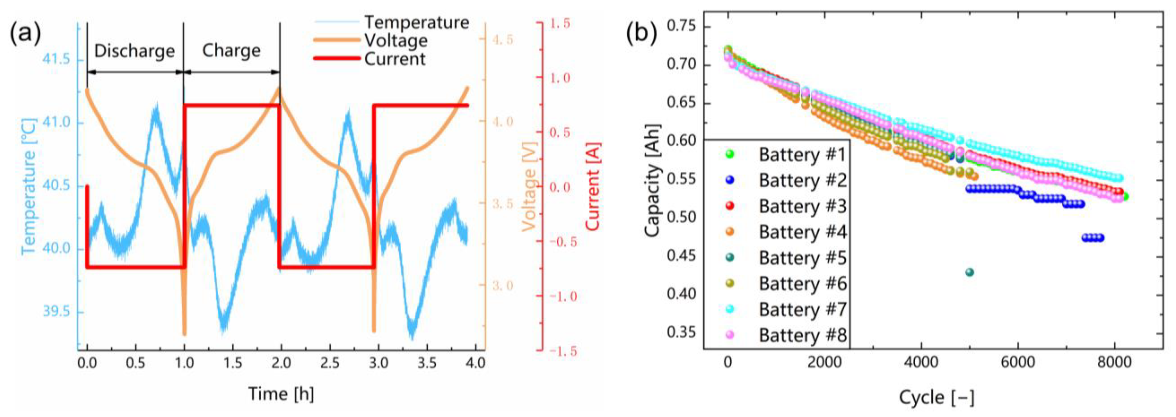
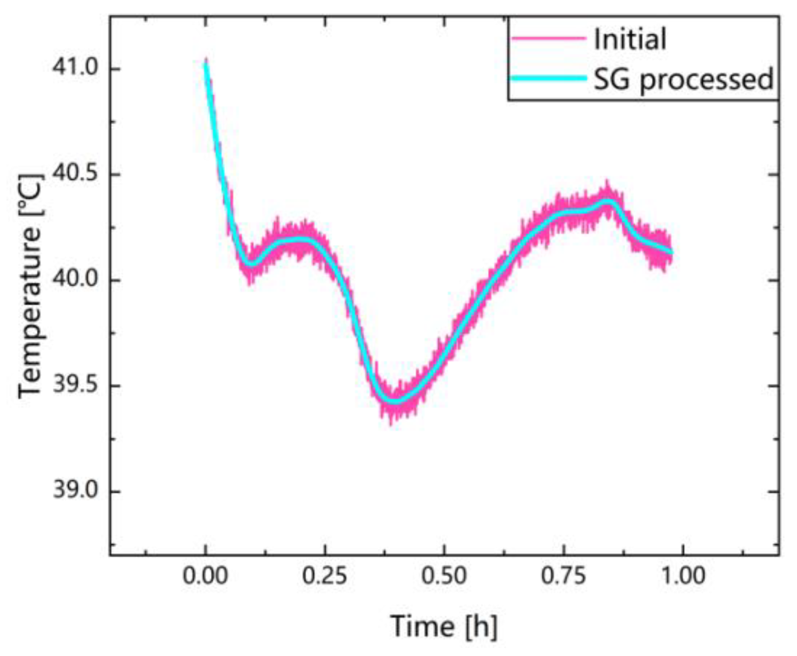
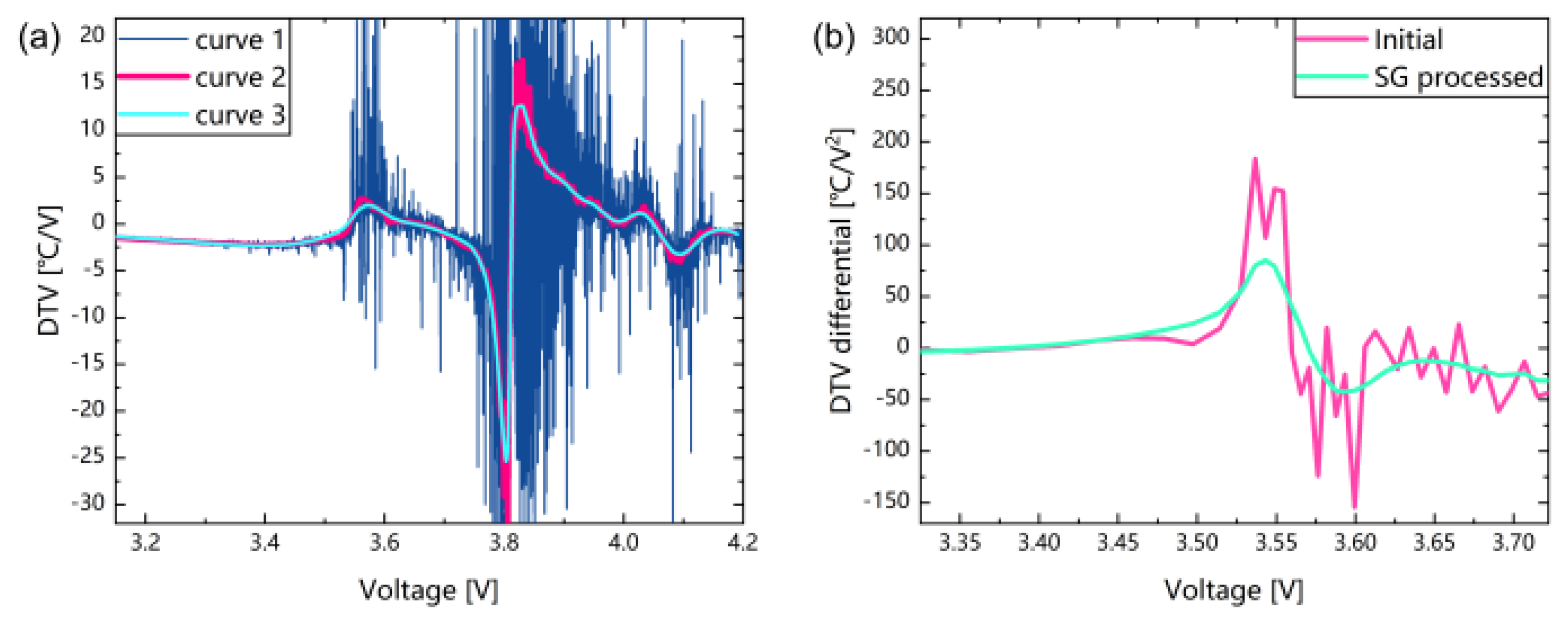
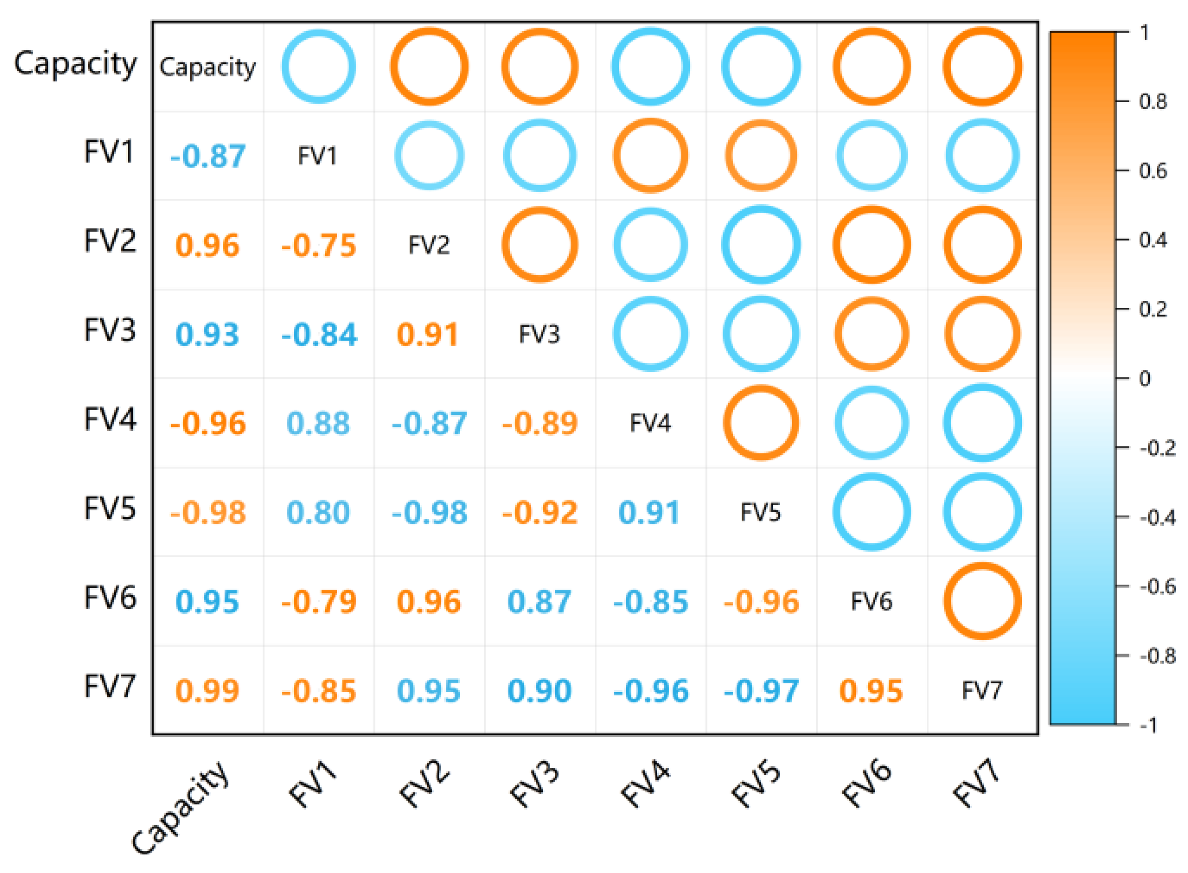
In this paper, the fusion of data-driven methods and feature signal analysis methods are proposed to realize early prediction of the SOH and RUL of high-energy density lithium-ion battery cathodes. To validate the proposed method, a data-driven model with LSTM network as the core and DTV feature signal analysis are utilized to construct the fusion model. Firstly, the DTV feature signal analysis is executed based on battery degradation data. With Savitzky-Golay (SG) filter method and Pearson correlation analysis, highly correlated features are extracted based on battery degradation datasets of Oxford University, including information of valleys and peaks from DTV curve and singular values of DTV vector, respectively. Next, a deep-learning model with LSTM network as the core is constructed and trained with these features. Furthermore, the dropout technique is introduced to solve the overfitting problems and the Monte Carlo simulation is utilized to characterize the prediction uncertainty. Finally, the model validation and error analysis are performed. This work demonstrate that features extracted from DTV curve could be utilized in deep-learning model to improve and optimize long-term SOH and RUL prediction based on the early degradation data. In framework of CHAIN, the proposed model could approach accurate offline SOH and RUL estimation or real-time online prediction combined with local fast empirical model, promoting the development of the next-generation cloud-vehicle synergistic management system [31,32,33,34].

2. Degradation Data

In this section, the DTV feature signal analysis is executed based on battery aging datasets from Oxford University [35,36]. With Pearson correlation analysis method, two kinds of feature variables are extracted as the input of subsequently established deep-learning model, including singular values from DTV vector and information of peaks and valleys from DTV curves, respectively.

2.1. Battery Aging Experimental Data

In this paper, the selected LCO/NCO battery degradation dataset is obtained from Oxford University based on 8 groups of 740 mAh pouch batteries (labelled from #1 to #8). The experimental batteries consist of graphite anodes, lithium cobalt oxide and lithium nickel cobalt oxide cathodes (LCO/NCO). There are 8 cells cycled through an 8-channel Big MPG 205 battery tester and housed in a MK53 hot chamber at 40 °C with constant current charge and discharge.

Table 1. Technical specifications and battery test procedures of the eight batteries.

Technical Specifications		Cycling Tests
Anode Material	Graphite	Charge test	CC charge at 2C
Cathode material	LCO/NCO
Nominal capacity [Ah]	0.74
Nominal voltage [V]	3.7
Discharge cutoff voltage [V]	2.7	Discharge test	Artemis drive cycle discharge
Charge cutoff voltage [V]	4.2
Weight [g]	19.5 ± 0.5

shows the specific parameters and experimental conditions. The C-rate is the measured value of charging or discharging current relative to its nominal capacity. The voltage, current and the temperature data recorded for two continuous cycles in the test are shown in Figure 1a. Figure 1b shows the battery capacity degradation curves of the 8 cells. At the end of the cycle test, the discharge capacity of battery #2 and #5 drop sharply. The surface temperature shows a clear change as well. Furthermore, the battery #6 does not reach below end of life (EOL). Therefore, the battery #1, #3, #4, #7 and #8 are selected and utilized for training and testing of our model.

2.2. Differential Thermal Voltammetry Analysis and Feature Extraction

2.2.1. Noise Removal

Noise will be generated in practical measurements due to fluctuations in signal sampling, especially temperature data, which is much louder than the voltage current data as shown in Figure 1a. Furthermore, the error caused by noise will be further amplified due to the differential operation and the obtained DTV curve will contain a lot of noise.

To address the effects of noise, in this work, our data was extracted from 1C constant current (CC) charge cycles in a characterization test with the time interval of 20 s. If the selected voltage measurement interval is too small, the noise will have a huge impact on the results of our test. If the selected voltage interval is too large, it may cause to the loss of valuable information. Therefore 20 s is chosen as the interval because the voltage interval is proportional to the time interval during CC charging.

After setting a fixed time interval, the DTV curves still contain a lot of noise. Therefore, the filtering method could be utilized to further process the data and we choose the Savitzky-Golay (SG) filter for smoothing. The SG filter is well-adapted for data smoothing as a type of low-pass filter. The filter method could maintain the shape and height of waveform peaks, which is suitable for filtering the DTV curves to obtain high-quality features [37]. The principle of filter could be described as follows:

$$y\left(i\right)={\displaystyle \sum }_{j=-p}^{j=p}\frac{1}{N_c}{C}_{j}x\left(i+j\right)$$

(1)

where $x\left(i\right)$ represents the original signals of input, $y(·)$ the synthetic signals of output, $C_j$ the coefficient given by the SG filter and $N_c$ the number of convoluting integers, which is equal to the smoothing window size (2p + 1).

Figure 2 and Figure 3 shows the comparison between the filtered battery surface temperature and DTV curve and the original curves obtained from the raw data. The DTV data as shown in Curve 2 in Figure 3a still contains noise, so they are filtered as well. The DTV curve contains obvious peaks and valleys, and the SG filter is suitable for preserving these important features of the the DTV curves.

The final graph is shown in Curve 3 in Figure 3a, which is the DTV curve we finally obtain. Due to the smoothness of the function is measured by continuous differentiation, Figure 3b shows our evaluation of the smoothing effect by deriving the DTV curve. As shown in Figure 2 and Figure 3, with the application of selected time intervals and SG filter, we could effectively smooth the original temperature curve and DTV curve and preserve the features on the curve well, including information of valleys and peaks.

2.2.2. Differential Thermal Voltammetry Analysis

The DTV method is an important tool for tracking battery health conditions, which could be utilized to evaluate the patterns of battery degradation process. The battery degradation is a complex physicochemical process. Therefore, the analysis of internal mechanism and measurement of parameters could be challenging. The change of entropy is a function of temperature, and the DTV method could provide obvious information related to entropy. Some feature variables, such as positions and heights of peak and valleys of the curve, are directly concerned with the impedance increment and nonuniform of electrode performance during battery degradation process, reflecting the phase transition characteristic. During the whole battery degradation process, the positive and negative electrodes are in different phase combinations. The transition between these phases may lead to a sudden change in entropy, which may lead to the emergence of inflection points on the DTV curve. Specifically, the peak position describes the peak potential during the (de) intercalation stage. The peak position shift during aging can describe the impedance rise and stoichiometric drift of the battery. The peak height represents the maximum heating rate of these stages. The peak width describes the potential window of the combined phase in the two electrodes. The peak area gives information about the heat generated during the (de) intercalation stage. The phase transition characteristic is closely related to the battery degradation, thus providing close links between DTV features and battery degradation.

The parameters of $DTV$ methods could be calculated by differentiate the temperature of the battery surface to the terminal voltage during charging, described as follows:

$$DTV=\frac{dT}{dt}/\frac{dV}{dt}=\frac{dT}{dV}$$

(2)

where $T$ represents the battery surface temperature, $V$ the battery terminal voltage. That is, we could obtain DTV only by obtaining temperature and voltage data from the battery during charging or discharging.

Figure 4 shows that the heights of peak will decrease, and the positions of peak will increase during battery degradation in charging process. Furthermore, the valley gradually becomes smaller and moves towards high potential. Obviously, the DTV method could help to reflect battery degradation characteristics by bridging microscopic phase transition characteristics and macroscopic signaling characteristics.

2.3. Features Extraction of Battery Degradation and Correlation Analysis

2.3.1. Features Extraction

As for the final obtained DTV curve, the characteristic information such as the position, size and width of the peaks and valleys is elected as alternative input features. These values are high correlated with the change in the impedance of the battery and are also direct or intuitive. The specific description of the peak and valley could be expressed as follows:

$$V_{peak}=V_i{}_{|\frac{dDTV}{d{V}_i}=0,andf\left(V_i\right)\ge f\left(V\right),V\in \left(V_{i-1},V_{i+1}\right)}$$

(3)

$$DT{V}_{peak}=f\left(V_{peak}\right)$$

(4)

$$V_{vally}=V_i{}_{|\frac{dDTV}{d{V}_i}=0,andf\left(V_i\right)\le f\left(V\right),V\in \left(V_{i-1},V_{i+1}\right)}$$

(5)

$$DT{V}_{vally}=f\left(V_{vally}\right)$$

(6)

where $f(·)$ is a mapping function between voltage and DTV, and $V_{i-1}$ and $V_{i+1}$ are the voltages of the previous sampling time point and the later sampling time point, respectively. As shown in Figure 5a, the coordinates of the first peak, the valley, and the second peak are [FV1, FV2], [FV3, FV4], and [FV5, FV6], respectively. In addition, FV1, FV2, FV3, FV4, FV5, and FV6 represent the values of $V_{peak1}$, $DT{V}_{peak1}$, $V_{vally}$, $DT{V}_{vally}$, $V_{peak2}$, and $DT{V}_{peak2}$, respectively. With the increase of aging cycle, the specific change processes of feature variables of battery #1 are shown in Figure 5b,c.

More attention is paid to the change of peaks and valleys for DTV feature signal analysis methods, but it is difficult to obtain accurate peak and valley information in the practical application process due to the influence of noise disturb, sampling intervals, electrochemistry and other factors, etc. Different measurement conditions could have a huge impact on the results. Even if accurate peak and valley information could be obtained, operations such as DTV curve smoothing, and peak and valley information feature extraction will increase the computational complexity of overall battery degradation estimation model.

Therefore, in addition to the commonly used peak and valley information as input features, we also selected the singular value decomposition method to extract the singular value of DTV data. The singular value decomposition is a simple and direct mathematical method, which can directly extract feature information from the unfiltered DTV data, avoiding the extra efforts of finding and extracting features from peaks and valleys of DTV curves, that is, singular value decomposition could reduce the complexity of data processing operation.

The principle of singular value decomposition could be described as follows:

$$M_{DTV}=U{{\displaystyle \sum }}_{DTV}{V}^T$$

(7)

where $M_{DTV}$ is the matrix of the l columns and k rows from DTV data. A column of DTV data could be seen as a matrix of k rows and l columns, where k is equal to the length and l is equal to one. After decomposition by SVD, it is split into 3 sub-matrices where the $U$ matrix is the square matrix of k rows and k columns, the $U$ matrix is the orthogonal eigenvector of the MMT matrix and $V$ is the square matrix of l rows and l columns. ${{\displaystyle \sum }}_{DTV}$ is a matrix with values only for the main diagonal, where the values are called singular values from DTV vector.

The singular values concentrate the important information of matrix in the larger singular values. The singular value decreases from the upper left from the largest to the smallest to the lower right at a very fast rate, so that the important information is concentrated in the upper left part of the ${{\displaystyle \sum }}_{\mathit{DTV}}$ matrix. In this paper, singular values are extracted for the DTV data of each cycle. The largest singular value is chosen as an additional feature FV7, and Figure 5d shows how FV7 changes with battery degradation.

2.3.2. Correlation Analysis

In order to improve the prediction accuracy and efficiency, the features with high correlation coefficient are selected through Pearson correlation analysis [38]. The formula of Pearson correlation analysis is described as follows:

$$r_{xy}=\frac{{{\displaystyle \sum }}_{i=1}^n\left(x_i-\overline{x}\right)\left(y_i-\overline{y}\right)}{\sqrt{{{\displaystyle \sum }}_{i=1}^n{\left(x_i-\overline{x}\right)}^2}\sqrt{{{\displaystyle \sum }}_{i=1}^n{\left(y_i-\overline{y}\right)}^2}}$$

(8)

where $n$ is the number of sample series, $x$ and $y$, respectively, represent a variable, and, respectively, denote mean values of $x$ and $y$.

The correlation analysis between the battery capacity and the features we extracted is shown in Figure 6. The correlation analysis results for all batteries are shown in

Table 2. Pearson correlation coefficients between feature variables and capacities.

Battery Label	FV1	FV2	FV3	FV4	FV5	FV6	FV7
#1	0.87	0.96	0.93	0.96	0.98	0.95	0.99
#3	0.91	0.92	0.94	0.96	0.96	0.91	0.97
#4	0.96	0.95	0.98	0.96	0.97	0.95	0.99
#7	0.95	0.94	0.89	0.91	0.98	0.92	0.94
#8	0.89	0.95	0.91	0.96	0.98	0.94	0.98

. It could be seen that the feature values we extract on different batteries have a high correlation with capacity and the correlation analysis results of most of the features are above 90%. The FV1 of battery #1 and the FV3 of battery #7 and the FV1 of battery #8 have reached more than 85%, though they have not reached 90%. Furthermore, the singular value features we extracted reached more than 94% on each of the four batteries. Finally, the features FV2, FV4, FV5 and FV7 are selected as the input features of the model. The FV2, FV4 and FV5 will be utilized as a set of inputs and FV7 will be used as another set of input datasets.

3. Methodology

This section mainly describes the framework of the proposed deep-learning method integrated of DTV analysis method and data-driven method.

3.1. LSTM Network Structure

LSTM neural network is a variant of RNN, which is suitable for long-term dependence problem and can effectively solve the gradient disappearance and gradient explosion problems. The LSTM introduces unit states and uses three types of gates, input gate, forget gate and output gate, to hold and control information. The main feature of the LSTM neural network is that there is a main chain of information recorded through the units, using the sigmoid function $\sigma (·)$ and the hyperbolic function $\mathit{tan}h(·)$ in each network unit, respectively [39]. Each unit of LSTM is described as follows:

The first step is to use the forget gate to determine which information is discarded from the unit state $c_{j-1}$ when the LSTM unit obtains the data for $x_j$ and $h_{j-1}$. The sigmoid activation function of the forgetting gate will output a number between 0 and 1, where “1” means that the status value is completely retained and “0” means that the value is completely discarded. This number will be utilized for update of unit status $c_j$. The forget gate can be expressed as:

$$f_j=\sigma \left(W_f\cdot \left[h_{j-1},x_j\right]+b_f\right)$$

(9)

Secondly, a sigmoid activation function and a $tanh$ activation function are used to form the input gate. The sigmoid function decides which values to update and then uses the tanh layer to obtain new information, consequently creating a new candidate state to participate in the update of unit state. These two steps could be described as follow:

$$i_j=\sigma \left(W_i\left[h_{j-1},x_j\right]+b_i\right)$$

(10)

$$g_j=\mathit{tan}h\left(W_g\left[h_{j-1},x_j\right]+b_j\right)$$

(11)

The third step is the fusion of data from the forget and input gates. Next, the unit state changes from $c_{j-1}$ to $c_j$:

$$c_j=c_{j-1}\times f_j+i_j\times g_j$$

(12)

The final output gate generates a new hidden state $h_{j-1}$ based on the unit state $c_j$.

$$o_j=\sigma \left(W_o\left[h_{j-1},x_j\right]+b_o\right)$$

(13)

$$h_j=o_j\times \mathbf{tan}h\left(c_j\right)$$

(14)

where the $W$ represents the weights of layer, b the deviations, $h_{j-1}$ the output of last cycle and $x_j$ the current output.

Since the battery degradation data is time-series data, recurrent neural networks (RNN) are well suited for the battery SOH and RUL prediction problems. Furthermore, battery degradation issue is a long-term dependency problem and general RNNs are only capable of solving short-term dependency problems. The problems of gradient disappearance and gradient explosion cannot be avoided as well, for which the LSTM neural network is utilized as the main body of the model in this paper.

3.2. Component and MC Simulation

In this paper, the optimization algorithm based on the RMSprop method is used to train the LSTM network. The RMSprop algorithm has been empirically proven to be an effective and practical algorithm for deep-learning neural network optimization. It works very well for RNNs, and is one of the frequently adopted optimization methods nowadays.

Neural networks suffer from overfitting problem, a phenomenon where the model performs well on the training datasets but poorly on the test datasets. The overfitting phenomenon will make the generalization ability and robustness of model deteriorate. Srivastava et al. proposed a dropout technique to solve overfitting problem more effectively [40]. During the training process, the dropout technique randomly removes neurons and their connections from the neural network. Whenever a dropout process is executed, it is equivalent to obtaining a smaller network from the original network consisting of the neurons left. Thus, training a neural network with the dropout technique can be considered as training many sparse networks with extensive weights sharing, where each sparse network is rarely trained. The network becomes less sensitive to the specific weights of the neurons, which allows the model to be more generalizable and not too dependent on certain local features.

Both the predicted values and their confidence levels are important parameters for assessing the performance of the predictor. The LSTM RNN is able to learn the long-term correlation of time series data and predict multi-step advanced data points, but it cannot provide prediction confidence. Therefore, we introduce MC simulation methods to characterize the prediction uncertainty. MC simulations require a numerical algorithm to describe the system. All information about the degradation process of battery performance is contained in the capacity datasets. Therefore, the LSTM RNN trained based on capacity data is defined as the numerical algorithm implemented by the battery degradation process, that is, the output of our LSTM model is utilized as the input data of MC simulations.

3.3. Input and Output Data Structure

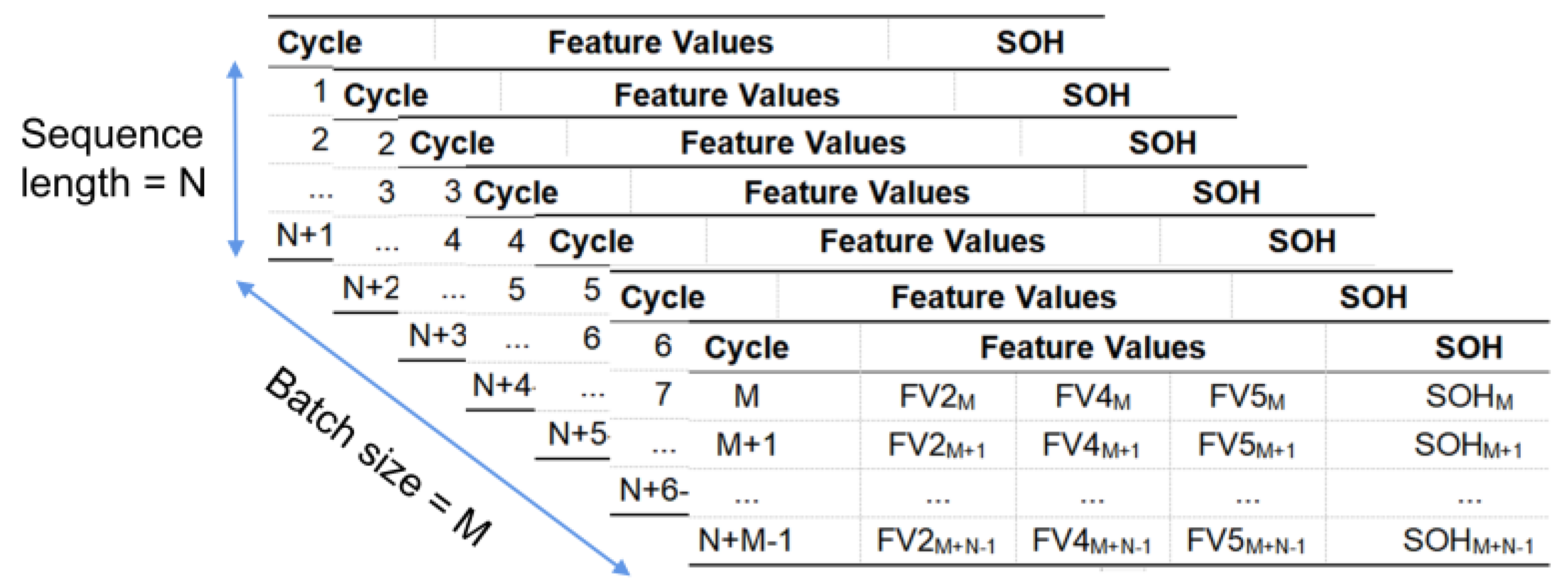
The specific structure of our inputs and outputs is shown in Figure 7.

Where FV represents features, M the batch size, SOH the capacity and N the sequence length. The timeseries are constructed using the extracted features and the input is constructed as a three-dimensional timeseries tensor. The extracted feature variables are first constructed into a two-dimensional matrix. Next, two-dimensional matrix fragments are extracted from the above two-dimensional matrix according to the sequence length N. Next, a series of two-dimensional matrix fragments are constructed into a three-dimensional tensor as the final input according to a given combination of batch sizes M. The features of each two cycles are used as a time series to predict the capacity of the second of these cycles, and the two adjacent timeseries will have an overlap of data points to make full use of our data.

3.4. Framework of the Proposed RUL and SOH Estimation Model

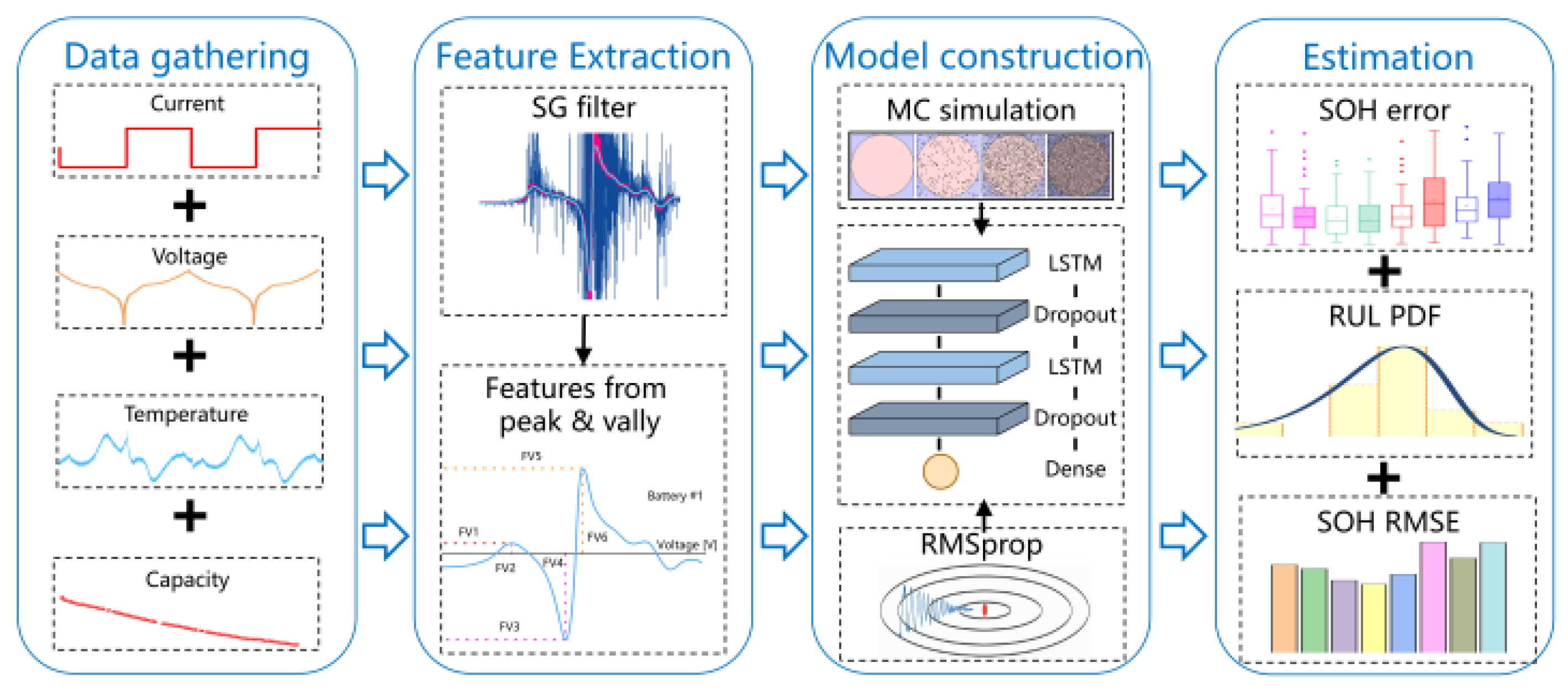
The specific framework of LSTM-based battery SOH and RUL prediction proposed in this paper is shown in Figure 8. The framework is divided into four parts: preprocessing, filtering and feature extraction, model construction and training, validation and error analysis.

In the first and second part, the data preprocessing and feature extraction are executed. As described in detail in Section 2, two kinds of features are extracted to train and test the deep-learning model, including information of valleys and peaks from DTV curves and singular values of DTV vector, respectively. In the third part, a deep-learning model with LSTM network as the core is constructed. The three-dimensional timeseries tensor obtained in the second part is utilized as input for training our model, and the RMSprop technique is used to improve the convergence speed during the training process. Furthermore, the Dropout technique is introduced to suppress overfitting and MC simulation is introduced to give uncertainty-related information in the computation process. Finally, the proposed battery health condition prediction model is quantitatively analyzed and validated. The mean absolute error (MAE) analysis, root mean square error (RMSE) analysis, and box plot analysis are utilized and compared. Furthermore, the proposed model is verified on the other four cells.

4. Result and Discussion

In this section, the validation and error analysis of our proposed model are executed. Different division proportions of the dataset are investigated firstly to ensure accuracy with a minimum amount of data, that is, approaching prediction of battery degradation early as soon as possible. Next, the robustness and stability of our model are proved and the accuracy of prediction results using singular values as input features of the model is calculated.

4.1. Experiment Setup

We use TensorFlow to build the whole network and use the compute unified device architecture (CUDA) to accelerate computation. The version of TensorFlow is 2.5.0 and the version of CUDA is 11.2. The overall experiment is performed on a server with AMD EPYC 7543 32-Core Processor CPU and NVIDIA A40 GPU, and the operating system is ubuntu 18.04.

The accuracy of the model and the training process are greatly affected by the hyperparameters in the LSTM network, which are pre-given rather than learned by the network. Batchsize determines the number of samples selected by the model in one training. The value of Batchsize will affect the optimization degree and speed of the model. A larger Batchsize will speed up the training speed, but it is easy to make the model converge at the local optimum point. After debugging, the Batchsize is selected as 2 is optimal. The value of the learning rate has a great impact on the training process. A large learning rate will cause the gradient to oscillate and may even fail to converge and a small learning rate will lead to a very slow convergence rate. After debugging, the learning rate is selected as 0.0012 as the best. Epoch represents the training times of all sample data. A large epoch will lead to slow model training and overfitting and a small epoch may lead to underfitting. In the experiment, it is found that convergence can be achieved by setting the epoch to 100, continuing training may lead to overfitting. Therefore, set the epoch to 100. The number of nodes in the network directly determines the performance of the network, too few nodes may lead to insufficient information processing capability of the network, which may lead to underfitting and too many neurons may lead to the limited amount of information contained in the training set being insufficient to train all neurons in the hidden layer, leading to overfitting. We debug in the range of 16–128, and the results show that 64 is optimal. Dropout rate is the probability of discarding neurons, too low probability has limited effect, while too high probability will lead to insufficient network training. After debugging, it is found that 0.2 is the best. The sequence length represents the length of the input sequence or the size of the input window, and sequence stride represents the step size of each sliding of the window. Due to the small amount of training data, in order to make full use of the training data, we set the sequence length to 2, and the sequence stride set to 1. The specific model structure and hyperparameters are shown in

Table 3. Specific hyperparameters and structure of model.

Criteria	Values
Species of layers	(LSTM, Dropout, LSTM, Dropout, Dense)
Units of layers	(64, -, 64, -, 1)
Dropout	20%
Activation Function	(tanh, -, tanh, -, sigmoid)
Sequence length	2
Batch Size	2
Epoch	100
Optimizer	RMS prop
Learning rate	0.0012
Training loss	Mean squared error

.

4.2. Validation of Early Prediction Ability

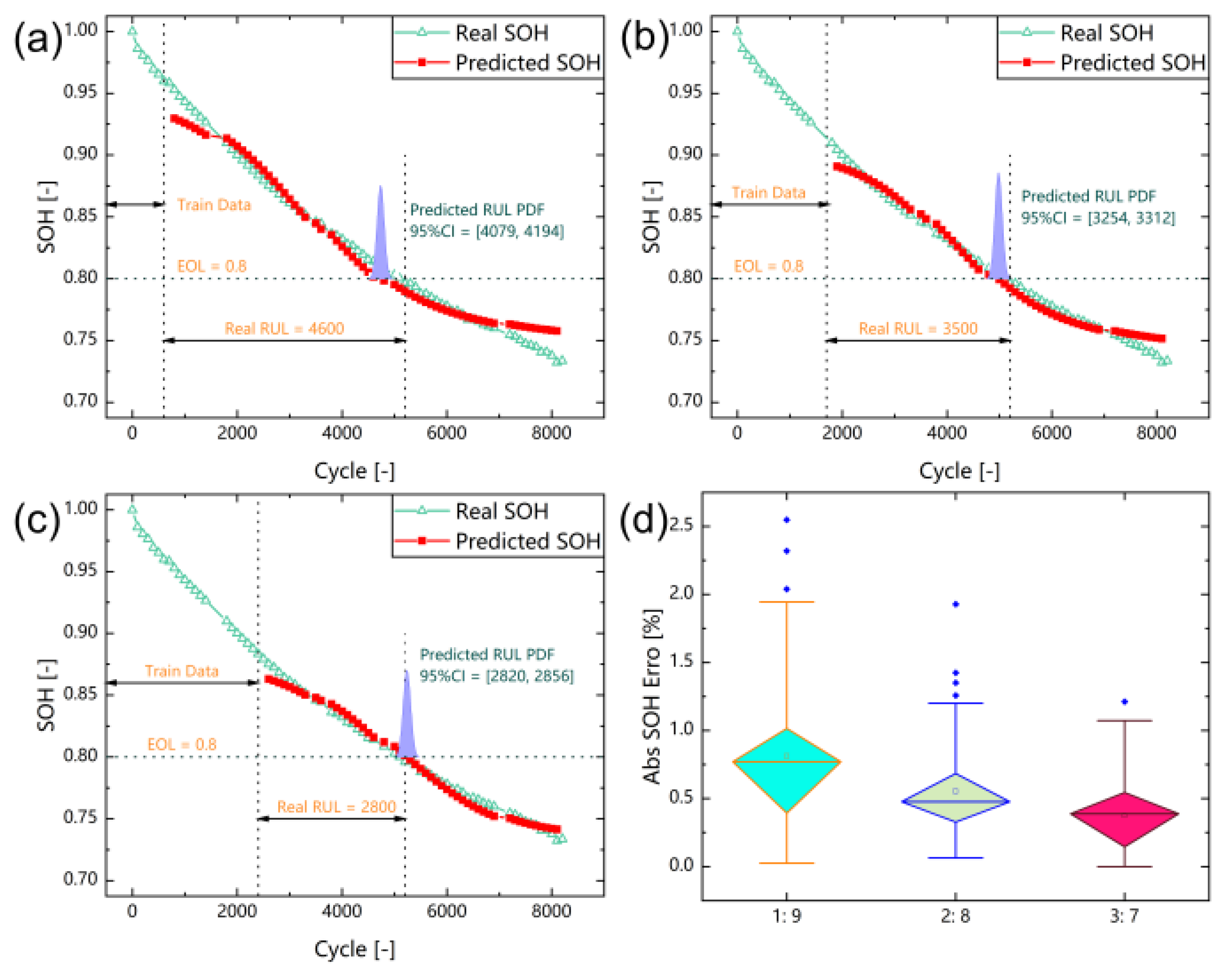
In this subsection, the variation of SOH and RUL prediction results with different division proportions of the dataset are investigated to verify the early prediction ability of the proposed model. The Red dotted line represents the predicted SOH and the green dotted line represents the real SOH. The division proportion is demonstrated with the black lines. The purple area is generated with Monte Carlo simulation to obtain the probability distribution of RUL. Three division proportions of dataset are executed in this subsection, including 10%, 20% and 30%, respectively. As shown in Figure 9a, the error of prediction is 0.714% when using 10% of data for training. The RUL is 4600 cycles, and the probability density of battery RUL is distributed between 4079 and 4194 cycles. Figure 9b shows that the error of prediction is 0.473% when using 20% of data for training. The RUL is 3500 cycles and the probability density of battery RUL is distributed between 3254 and 3312 cycles. The precision is significantly higher than the results using 10% of data for training. Figure 9c shows that the error of prediction is 0.363% when using 30% of data for training. The RUL is the 2800 cycles, and the probability density of battery RUL is distributed between 2820 and 2856 cycles. Figure 9d shows the box plot of the predicted results, which avoids the effect of extreme outliers and provides a visual table of the error distribution conditions with small rectangles in each box representing the MAE. The box plot could show the characteristic of the error distribution through maximum, minimum, median, upper quartile and lower quartile. With the proportion of the training set increasing, the upper quartile gradually decreases from 1.1% to 0.75% and to 0.5%, and the lower quartile gradually decreases from 0.4% to 0.25% and to 0.15%. The MAE also decreases from 0.8% to 0.6% and to 0.3%.

When using 30% of data for training, though the error is lower and the probability density distribution of RUL is closer to the real failure cycle, the predicted RUL interval is distributed after the actual failure cycle. The accuracy of prediction result using 20% of data for training is slightly lower than that of using 30% of the results—and the predicted RUL intervals are distributed before the actual failure cycle. At the same time, under the strict condition that only 10% of the data is used for training, and the dataset is in 100 cycles, which may lead to some missing information and have an impact on the accuracy. However, the model accuracy is still decent with a prediction error of 0.714%. Therefore, the results indicate that our method could achieve early SOH estimation and RUL prediction, that is, the proposed model could ensure high enough accuracy with the least amount of data for training.

4.3. Validation of Robustness

In this subsection the robustness and reliability of the proposed model is investigated. Some of the eight battery capacity data did not reach below EOL, making it impossible to derive RUL predictions. Therefore, the battery #3, #4, #7 and #8 are selected for verification. The red dotted line illustrates the predicted SOH and the green dotted line illustrates the real SOH. With Monte Carlo method, the probability distribution of RUL is obtained as the purple part. In these validations, the first 20% of the data are used as training dataset, and the cycle after is used as the starting cycle for prediction.

Figure 10 shows the validation of the robustness and reliability of the model using the commonly chosen information of peaks and valleys as features. The proposed method is validated on all four cells and the prediction errors are distributed around 0.4%. As shown in Figure 10a, the RUL is 2900 cycles, and the probability density of battery RUL is distributed at 2700 cycles for battery #3. Figure 10b shows that the RUL is 2500 cycles and the probability density of battery RUL is distributed between 2418 and 2469 cycles for battery #4. Figure 10c shows that the RUL is 4300 cycles, and the probability density of battery RUL is distributed between 3932 and 3968 cycles for battery #7. Figure 10d shows that the RUL is 3000 cycles and the probability density of battery RUL is distributed between 2950 and 2984 cycles for battery #8. It could be seen that the predicted RUL probability densities do not cover the actual effectiveness cycle very precisely, but they are distributed in a small interval close to practical failure cycle. The reason for not covering the practical failure cycle may be that the original dataset is in 100-cycle increments, which may result in some information missing.

As shown in Figure 10e,f, the prediction results with the data of 20% cycles lost could produce a prediction mean absolute error of around 0.4%, which is close to 0.473% without data lost. Furthermore, the lower and upper quartiles and MAE of box line plot are distributed around 0.25%, 0.6% and 0.75%, respectively, further proving the robustness and stability of our model.

4.4. Predict Result with SVD Feature

In this subsection the singular values are utilized as the input features for training and the four batteries are utilized to verify the verify the proposed model. Furthermore, all of the prediction results of SOH and RUL are obtained with data of 20% cycles lost. The red dotted line and the green dotted line represent the predicted SOH and real SOH, respectively. The purple area demonstrates the probability distribution of RUL, obtained with Monte Carlo simulations.

Figure 11 shows the prediction results using the singular values of DTV vector as features. As shown in Figure 11a–d, the prediction results with data of 20% cycles lost could produce a prediction mean absolute error of around 0.4%, which shows that the accuracy of prediction using singular values of DTV vector as features is slightly lower. However, the singular values can be extracted directly from the original DTV data without complicated operations such as filtering, and the accuracy is high enough for practical application. Furthermore, the predictions in this section using the singular value as features are taken as the starting point of 20%, which proves the robustness and reliability of using singular values as features as well.

Figure 11e,f shows the results of the box plot and the error analysis of the model. The lower quartiles are all distributed around 0.3% and both MAE and RMSE are distributed at the same level. The upper quartile using singular values as features for battery #7 and #8 reaches 0.8%, and the MAE and RMSE reach around 0.6% and 0.7%, respectively. It can be seen that it is feasible to extract the singular values of DTV data as features for prediction, and could make the process simpler with comparable accuracy. Figure 11 shows the results of the prediction using the singular values of DTV as features and the error is slightly larger than the results for other batteries, which is caused by the inconsistency of batteries.

Generally, the singular values have a strong correlation with the capacity data, which could encompass the information of peaks and valleys as an independent set of feature inputs. The prediction results using singular values as input features could produce a tolerable error. Furthermore, the utilization of singular value decomposition for DTV enables the use of simpler data processing and feature extraction methods to extract strongly correlated features. The singular value could replace the peak-valley information, reducing the size of input matrix and improving the efficiency of the model.

4.5. Validation of Computation Cost and Compared with Other Methods

Table 4. Computation cost of training and prediction.

Battery Label	Data Start	Data Split Portion	Feature	Training Time(s)	Prediction Time(s)
#1	0%	1:9	2, 4, 5	19.047	0.698
	0%	2:8	2, 4, 5	20.661	0.637
	0%	3:7	2, 4, 5	21.800	0.611
	0%	2:8	7	19.979	0.576
	20%	2:8	2, 4, 5	20.119	0.741
#3	20%	2:8	2, 4, 5	18.729	0.582
			7	18.234	0.517
#4	20%	2:8	2, 4, 5	16.367	0.706
			7	17.450	0.561
#7	20%	2:8	2, 4, 5	19.079	0.571
			7	19.000	0.577
#8	20%	2:8	2, 4, 5	18.961	0.552
			7	18.493	0.525

shows the computation cost of training and prediction. As shown in Table 4. The training time is about 20 s, and the prediction time is about 0.5 s. The results show that the method proposed by us has low calculation consumption and high calculation efficiency. The computation cost of deep learning models in training is usually huge, and will increase dramatically with the increase of data volume. The high calculation efficiency of our proposed method is benefit from extracting features from DTV data, which reduces the amount of data, and using correlation analysis methods to further filter features, which reduces the number of features. At the same time, the amount of data we use is inherently small, and we have achieved high-precision prediction under the premise of using small amounts of data, which further proves the superiority and effectiveness of our proposed method.

Table 5. RMSE of SOH estimation result.

Method	Data Start	Data Split Portion	Feature	RMSE(%)
				#1	#2	#3	#4	#5	#6	#7	#8
Ours	0%	1:9	2, 4, 5	0.714	-	-	-	-	-	-	-
		2:8		0.473	-	-	-	-	-	-	-
		3:7		0.363	-	-	-	-	-	-	-
		2:8	7	0.582	-	-	-	-	-	-	-
	20%	2:8	2, 4, 5	0.433	-	0.390	0.324	-	-	0.347	0.415
			7	-	-	0.373	0.308	-	-	0.485	0.480
SVR [41]	0%	Leave-one-out cross validation	dT	1.43	2.81	1.08	1.50	3.62	1.17	1.80	1.39
			ICA	0.65	0.97	0.45	0.41	3.51	0.23	0.40	0.49
Random forest [42]			CCCT	0.47	0.97	0.36	0.44	0.44	0.37	0.66	0.42
SVM [43]			Voltage Temperature ICA	0.85	2.33	0.75	0.58	0.64	0.93	0.59	0.57
MLR [43]				0.84	2.02	0.73	0.55	0.60	0.97	0.37	0.43
GPR [43]				0.94	2.11	0.81	0.45	0.51	0.94	0.53	0.62
Fusion of SVM MLR GPR [43]				0.70	0.79	0.57	0.42	0.48	0.86	0.51	0.51
GRU [44]		Train: #1 #2 #3 #5 #6 #7 Test: #4 #8	Voltage	-	-	-	1.43	-	-	-	0.88
CNN [44]				-	-	-	1.24	-	-	-	1.56
GRU-CNN [44]				-	-	-	0.61	-	-	-	0.65

shows the prediction results of the proposed method in this paper and compared with other works that have also conducted studies based on Oxford battery dataset. This research have utilized traditional machine learning algorithms and some hybrid algorithms to build battery degradation models. Most of their input features come directly from voltage and temperature data or use ICA methods to extract features, rather than DTV data used in this paper. The model with support vector regression (SVR) as the core is constructed, with dT and ICA as the features, respectively [41]. A model with random forest as the core was constructed, and constant current charging time (CCCT) was taken as the feature [42]. Support vector machine (SVM), multiple linear regression (MLR) and gaussian process regression (GPR) are used as the core to build models, respectively, and the three models are fused through the random forest algorithm, with voltage, temperature and ICA as the characteristics. Ref. [43] establish models with CNN and gate recurrent unit (GRU) as the core, respectively, and the final output of the two models concatenated and projected to the output to build a GRU-CNN model, and the features are extracted from voltage. Ref. [44] compared with most prediction methods in the table, the method designed in this paper has higher SOH prediction accuracy. It benefits from the input characteristics provided by DTV analysis and the excellent ability of LSTM network to solve long-term dependent time series problems. At the same time, we use less data as the training set, which further proves the superiority of this method. The comparison results show that the designed SOH prediction method has good prediction performance.

5. Conclusions

In this paper, the fusion of a data-driven method and a feature signal analysis approach is investigated to predict the SOH as well as RUL of battery cathodes. The DTV feature signal analysis is calculated based on the collected battery voltage and temperature information. Two kinds of features are extracted as the input features of the data-driven model from DTV data, including the singular values of the DTV vector and the peaks and valleys information of DTV curves, respectively. Subsequently, a deep-learning model is constructed with LSTM network as the core. Furthermore, dropout method is utilized to suppress overfitting and MC method is introduced to give uncertainty-related information.

Different division proportions of the dataset are investigated firstly. The results show that the prediction accuracy improves significantly with the increase of training set. However, 20% of the data ensures both accuracy and uses the relatively less amount of data with the prediction error of SOH maintained 0.473%, which is the best choice as a training set during early prediction. Next, the robustness and reliability of the proposed model are validated by removing the first 20% of the data for different start-up cycles. The prediction error of SOH is 0.433%, which is very close to the prediction error of 0.473% without data loss. Finally, the singular values are utilized as input features with the prediction SOH error of 0.582%, which is slightly higher than the error of 0.473% but can reduce the complexity of data processing while ensuring the prediction accuracy.

The main contributions of this work could be described as follows. (1) The DTV curve, which can characterize the phase-transition electrodes, is obtained and used to analyze the battery degradation process by cleaning, reducing, filtering and processing the raw voltage and temperature data. (2) Two kinds of features are extracted, and the singular values are simpler, reducing the cost and decreasing the computational complexity. (3) Only a small portion of data from early battery cycles is used for model training to achieve high accuracy of battery RUL prediction. (4) The robustness and reliability are investigated and validated with the data of 20% cycles lost. Generally, the proposed LSTM-based model has good early prediction accuracy and robustness, proving that the fusion of data-driven methods and feature signal analysis methods has good prospects for application in electrode health conditions estimation. This work could improve the prediction accuracy and has potential to approach cloud-end highly accurate offline prediction and achieving local-end real-time accurate estimation of SOH and RUL combined with local fast model in CHAIN.