Abstract
The concept of Digital Twin (DT) is widely explored in literature for different application fields because it promises to reduce design time, enable design and operation optimization, improve after-sales services and reduce overall expenses. While the perceived benefits strongly encourage the use of DT, in the battery industry a consistent implementation approach and quantitative assessment of adapting a battery DT is missing. This paper is a part of an ongoing study that investigates the DT functionalities and quantifies the DT-attributes across the life cycles phases of a battery system. The critical question is whether battery DT is a practical and realistic solution to meeting the growing challenges of the battery industry, such as degradation evaluation, usage optimization, manufacturing inconsistencies or second-life application possibility. Within the scope of this paper, a consistent approach of DT implementation for battery cells is presented, and the main functions of the approach are tested on a Doyle-Fuller-Newman model. In essence, a battery DT can offer improved representation, performance estimation, and behavioral predictions based on real-world data along with the integration of battery life cycle attributes. Hence, this paper identifies the efforts for implementing a battery DT and provides the quantification attribute for future academic or industrial research.
1. Introduction
Digital Twin (DT) is a virtual dynamic model of a system, process, or service, with real-world data interactions that facilitate improved system analysis and comprehensive representation [1]. NASA defined DT as an integrated multi-physics, multi-scale simulation of a system that uses the best available physical models, sensor data, and historical data to mirror the life of its physical twin [2]. The applications of DT are: (1) to simulate the behavior of the physical twin before its usage, where even without the benefit of continuous sensor updates, the DT can study the effects of various parameters, determine the various anomalies and validate the degradation mitigation strategies; (2) to simulate the system behavior during operation, through the continuous update of actual load, temperature, and other environmental factors, as input to the models, enabling continuous predictions for the physical twin; (3) to perform diagnostics in the event of a fault or damage; (4) to serve as a platform where the effects of parameter modifications, not considered during the design phase, can be studied. In practice, DT implementation involves allocating real-world data to the virtual model or platform. Boschert et al. [3] identified that simulation would become the primary tool for decision support once a DT is fully integrated. Likewise, Kunath et al. [4] summarized the three main functions of a DT: Prediction—execution of studies ahead of the system run; Safety—monitoring and control of the system state in terms of a continuous prediction during the system run; Diagnosis—analysis of unpredicted disturbances during the system run.
By definition, a model is a simplified abstraction of the structure or processes that define a real system. In that sense, models do not aim to replicate the original system in intensive detail [5]. The idea of moving a digital model closer to the real system is in fact a basic rationale for building computer models. Some models are extreme simplifications of the real system, while some are much closer to the real system, through multiscale simulations and interdisciplinary collaborations. The difference between a DT and a simulation model has been discussed previously [1,6], but it is essential to address the features that qualify a model as a DT: (1) model of the product—physical or data-driven; (2) evolving set of real-world data about/related to the product; (3) method of adjusting the model in accordance with the data. According to [7], the DT evaluation framework consists of four metrics, autonomy, intelligence, learning, and fidelity.
Some articles [8,9] describe seemingly similar concepts to DTs, such as digital shadow, virtual model, product avatar and digital thread, but they do not necessarily indicate the complete concept of DT, but rather fragments of overlapping functions. DT implementation is often mapped to IoT (Internet of Things) devices and CPS (Cyber-Physical Systems) [10,11], due to its high dependence on a compatible mode of data acquisition. A DT can have single or multiple stakeholders and may make use of 3D simulations, IoT devices, 4G and 5G networks, blockchain, edge computing, cloud computing, and artificial intelligence. Depending on the complexity, a DT may have access to past and present operational data along with predictive capabilities.
A multitude of literature [12,13] has been published, defining and characterizing the concept of DT in a variety of domains. However, missing from the literature is a consistent view on what the DT is and how the concept is helping to meet the challenges of the many use-cases to which it is being associated as a solution approach [14]. Some articles [15,16,17] suggest the methodologies, frameworks, and interpretation of DT for specific use cases. While this may help understand the system boundaries, it also leads to inconsistent ideas of the requirements of DT implementation and thus generating the risk of diluting the concept. The potential costs, infrastructure challenges, clarity of return on investments for product/process DT are not transparent. Without substantial effort to describe and quantify the DT benefits, it is challenging even to suggest that the concept itself may be the most appropriate solution to the challenges faced by each particular industry [14].
DT is generally perceived with the core idea that it is a model that can replicate the behavior of an existing system through the acquisition of real system data. This highlights the importance and completeness of the phrase “replicate the behavior”. To which extent is the replication satisfactory? DTs at first may appear to be a replica but replicating every behavioral aspect might not necessarily be realistic. For example, in battery DTs, it is unnecessary to digitally replicate each of the molecular, fluid, and structural behavior of each cell component. DTs need not attempt to mirror everything about the original system [5]. Hence, the reality of an exhaustive high-fidelity DT, which replicates every aspect of the physical system and maximizes services while minimizing expense and technical difficulty of implementation, is ambiguous. The level of model fidelity, cost, and effort for implementation is subject to limitations which will vary depending on the use case and its applications. Furthermore, the idea of DTs across the lifecycle is not yet fully understood. The number of DTs required across the entire lifecycle, or the transitions and interactions between the software components of the DT are yet to be explored.
Therefore, the stakeholders in industries or academia looking to invest in or develop a DT face the following challenges:
- Limited use cases and implementation results available to learn from others;
- No clear guidance on how much to budget;
- Difficult to know where to start to get value quickly;
- Initiatives that are misleadingly branded as “Digital Twin”;
- Limited know-how.
The hypothesis that DT would be a driver for product lifecycle management and smart manufacturing in the future needs to be tested. This paper is a part of an ongoing study that investigates the DT functionalities and quantifies the DT attributes across the life cycle phases of a battery system. Essentially, the pressing question is whether battery DT is a practical and realistic solution to meeting the growing challenges of the battery industry, such as degradation evaluation, usage optimization, manufacturing inconsistencies, second-life application possibility, etc. Within the scope of this paper, the concept of DT will be explicitly explored for battery cells and the functionalities it can offer during the operation and end-of-life (EoL) phases. Research on battery DT has already gained much popularity, and with this paper, we aim to provide a consistent approach to DT implementation for battery cells. In doing so, we identify the efforts for implementing a battery DT. The contributions of this paper are as follows: (1) literature-analysis of the potential functionalities of a battery DT during operation and EoL; (2) battery DT implementation approach; (3) KPIs (Key Performance Indicators) to quantify the value-add of battery DTs; (4) testing the main functions of the implementation approach on a DFN model.
This paper is structured as follows: Section 2 reviews past literature followed by a discussion about battery DT functionalities during operation and EoL. Section 3 outlines the approach of battery DT implementation with subsections elaborating each step. Section 4 demonstrates the results of the application of the described approach in Python. Lastly, Section 5 and Section 6 is a discussion of the contributions of the paper and its future scope.
2. Battery DT Functionalities during Operation and End-of-Life
The number of literature specific to DTs has increased drastically in the last decade [8,18]. The topic is explored in various domains, such as product optimization, production planning/control, layout planning, maintenance, or product lifecycle. However, a microscopic look into the implementation of product DT, i.e., battery DTs has become prevalent since the past decade with increased utilization of IoT devices, CPS, and cloud-based services. Sometimes battery model implementation learns from real-time operational data to evaluate the battery states but is not necessarily defined as a battery DT [19]. So, is it crucial to even understand if a model is, in fact, a DT? Generally, at the initial stage of product development, it is not an essential requirement. However, at the business level i.e., in order to draw profits and innovation in the existing business model, a DT can facilitate effective R&D.
In the context of battery systems, it is uncertain whether battery DT insinuates a single cell DT, module-level DT, or pack-level DT. Currently, DTs are the result of custom technical solutions that are difficult to scale [20]. The scalability of battery DTs depends on the extrapolation of cell behavior through physical, physics-based, or data-driven battery models. For this purpose, the term battery DT referred to in this paper implies the DT of a battery cell. However, module and pack-level battery DTs are worth pursuing in the later stages.
The literature review in this paper takes only those published literature into account, which consists of practical implementations of battery DTs with defined DT-functionalities and implementation methods. The focus is on reviewing the latest literature on DTs concerning applications in the battery industry, published in the past 5 years (starting from 2016 to 2021). With Google Scholar as the research literature database and the following logical expression of keywords: (“digital twin”) AND (“battery”) AND (“lithium-ion”), updates until July 2021, the total number of resulting articles were 392 (39 google scholar pages), among which several articles had to be excluded due to the following reasons:
- Some articles only mentioned battery DTs as a possible application
- Some of them did not explain the architecture to support battery DTs
- Others were only theoretical articles.
However, in combination with advanced search for the keywords (“battery digital twin”) or (“digital twin” AND “battery”) in the title, the literature was filtered down to 9 articles. As a result, Table 1 elaborates the available literature, their reported method of DT implementation, and the corresponding DT functionality.

Table 1.
Literature review of DT-implementations relevant for battery system.
While some of the references identified in Table 1 are pioneering attempts to map real-time battery data to the battery models through cloud services, the others have yet again used simulated driving cycle data to validate the state estimation algorithms. This procedure of using drive cycle simulations such as WLTP (Worldwide Harmonized Light Duty Vehicles Test Procedure) or UDDS (Urban Dynamometer Driving Schedule) for validation of battery state estimation algorithms is a state of the art state estimation approach [30]. Nevertheless, this is not ideal for designing battery DT because simulated driving cycles can only validate the algorithm accuracy of static models while battery DTs are dynamic. Additionally, a common observation among all the DT functionalities in Table 1 is that they all have approximately the same output, i.e., SOC, SOH, internal resistance, or capacity. Evaluation of the battery state through these output variables has already been an established requirement from electrical models, electric-thermal models, electrochemical models, and until recently, data-driven (or NN) battery models. In this context, it is worth noting the conundrums that this raises regarding the argument about the need for a battery DT only for performing state estimations. Other than the fact that if implemented correctly, a battery DT should deliver those output variables to the users, developers or testers in real-time, there are no significant utilities that only a battery DT can implement. So, what additional value-add does a battery DT contribute? In an attempt to answer this, the following 2 aspects are now elaborated:
- Battery DT influence on life cycle phases;
- Current BMS functionalities.
To achieve competitiveness with the internal combustion engine, the key requirement for battery development is high driving ranges, low-charging times, and low battery pack cost. The performance indicators of batteries during usage are characterized by cost, specific energy (Wh kg−1), energy density (Wh L−1), specific power (W kg−1), and power density (W L−1), and charging time (=fast charging ability) [31]. While a DT cannot take the responsibility of improving the energy density or specific power of a battery, it can significantly aid the design optimization process and EoL assessment process. Sensing the battery data and uploading that to a storage server gives the opportunity to easily access the battery data and create learning models, which directly guide the product design, and optimization process [27]. The battery data storage platform stores the design and usage history, which supports behavioral integration in consequent life cycle phases and simplifies the prediction of the remaining useful life (RUL) during operation and also at EoL for second life assessment [32].
The Battery Management System (BMS) is the central element for protecting, monitoring, and controlling the battery-powered system by ensuring safety, efficiency, and reliability [33]. BMS measurements are performed for cell voltages, pack current, pack voltage, and pack temperature and it usually uses these measurements to estimate SOC, SOH, DOD (Depth of Discharge) [34]. Battery DT requires the onboard-BMS to work together with the battery data storage platform.
The potential functionalities of a battery DT in combination with an onboard-BMS are identified in the literature. Identifying the stress factors from the time-series measurement data and calculating its effect on the model parameters facilitates evaluating battery aging indicators during operation [25]. Besides, the model update integrated with the charging data enables a battery DT to maximize the optimization objective and select the best parameters for an optimal charging strategy such as multi-stage constant current charging, pulse charging, multi-stage constant heat charging and AC charging [35]. Similarly, thermal management based on battery DT relies on prediction of aging effect of temperature distribution across the battery pack using thermal models. Detection and traceability of sensor faults, electrical faults, and thermal runaway in a battery DT can allow integration of fault diagnosis procedure of the BMS with the battery DT functionalities [32].
In order to identify the functionalities and potentially the value add of a battery DT, the above discussion is encapsulated in Figure 1. The black circle lists the functionalities of a BMS, taken from the datasheets of two commercial BMSs found in [36,37]. The extended blue block lists the battery DT outputs taken from Table 1. These are the applied battery DT functionalities. Lastly, the green block lists the potential DT functionalities identified from the literature (as highlighted above). Thus, Figure 1 compares the existing BMS functionalities with the applied battery DT functionalities and the potential battery DT functionalities.
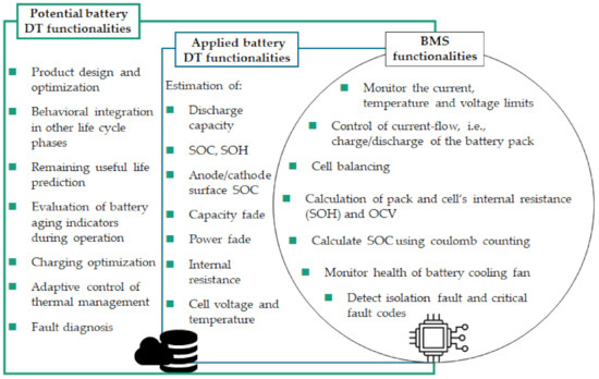
Figure 1.
Comparison of BMS functionalities with the applied battery DT and the potential battery DT functionalities.
The BMS functionalities taken from the referenced datasheets are to monitor the current and temperature sensors. It uses programmed settings to control the current flow into and out of the battery pack by broadcasting the charge and discharge current limits, cell balancing, and monitoring each cell tap to ensure that cell voltages are not too high or too low. Using the programmed values in the battery pack profile, the BMS calculates the pack and individual cell’s internal resistance (SOH) and OCV. Current sensor data is used to calculate the battery pack’s SOC (via coulomb counting CC).
The SOC estimation method in the studied BMSs is CC. Literature shows alternative methods with higher estimation accuracy, such as adaptive EKF, impedance method, fuzzy logics, SVM, hybrid method (EKF combined with ANN) [38,39,40]. Here a DT can complement the current BMS functionalities by applying estimation algorithms with higher accuracy. Moreover, the main functionality of the BMS is to ensure that the battery stays with its specified limits. It takes immediate measurements to analyze the voltage and temperature of the cell to estimate the SOC. It does not consider the degradation effect of the charge/discharge cycles on the battery from an electrochemical perspective. The immediate battery user may not be interested in understanding the degradation effects of the battery, such as loss of lithium, diffusivity of electrolyte or SEI resistivity at the anode. However, for deeper knowledge and future innovations by the battery designers, this would serve as a stepping-stone towards ensuring that the battery lasts until its maximum possible capacity and optimal performance. Hence, a DT can complement the functionalities of a BMS by taking the load for large computation requirements. BMS diagnostics over a long period can be enhanced and even simplified by using a DT.
To sum up, the added value that battery DTs can offer is improved representation, performance estimation, behavioral predictions, optimization strategies, and integration of battery life cycle attributes to the remaining DT functions.
3. Approach
In this section, an approach for implementing a battery DT is introduced. The purpose is to define a functional procedure to move from battery model to battery DT systematically. Figure 2 illustrates the 5-step approach, and each step is then further elaborated. By piecing together the existing methodologies of battery modeling, model parameter estimation, battery state prediction, the efforts needed for implementing a battery DT will be investigated.
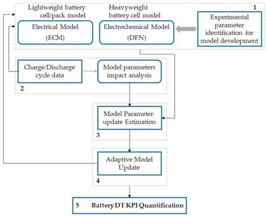
Figure 2.
Approach for battery DT implementation.
3.1. Step 1: Lightweight or Heavyweight Battery Model Development
The first step to implement a battery DT is inevitably the development of a reliable battery model. Battery models have become an essential tool in battery-powered applications, which are safety and performance-critical. Depending on how the model inputs and outputs are related, battery models can be classified as empirical, semi-empirical, physical and, data-driven [41,42], while the different types of battery models are:
- Electrical model (ECM);
- Electrochemical model (P2D);
- Thermal model;
- Mechanical model;
- Interdisciplinary combined model.
Fast and accurate identification of the BMS model parameters is a vision for battery developers and engineers. With the outlook of computational expense, the battery model types can be differentiated as either lightweight battery models or heavyweight battery models. Based on [43], the factors which differentiate between the two are as follows:
- Battery dynamics represented by the model
- Number of parameters
- Computation time
- Accuracy
- Ease of understanding and complexity for implementation.
We limit discussion to only electrochemical and electrical models for this paper. As a lightweight model, ECM of a battery is relatively easy to scale to the module or pack level and is widely used in BMS algorithms. They are derived from the empirical measurements of external characteristics of the cell [44]. However, by observing only the external behavior of the battery, the internal electrochemical dynamics cannot be entirely represented, and it is challenging to provide insights into electrochemical or life-reduction phenomena occurring inside the battery. Additionally, ECMs are developed based on data obtained from specific operating conditions of the target batteries, and their accuracy abruptly decreases while performing calculations on other operating conditions or if the battery is replaced [45].
As heavyweight models, the electrochemical models mainly fall into two categories, single particle model or pseudo two-dimensional (P2D) model (also known as the Doyle-Fuller-Newman—DFN model). DFN model for lithium-ion batteries use the combination of the porous electrode theory and the concentrated solution theory [46]. Compared to ECM, which has less physically relevant parameters, a DFN model contains a large number of parameters with a physical meaning. It calculates electrical, chemical, and electrochemical phenomena occurring inside the battery to predict its performance and lifespan Hence, DFN models provide the opportunity for a deep understanding of lithium-ion batteries’ aging mechanisms, accurately predicting battery performance by considering the material characteristics and the electrode design.
Experimental Parameter Identification Techniques
Accurate fitting of the battery model with experimental data is not the focus of this paper, so the authors rely on the existing techniques. Instead, the focus is parameterizing the model once the battery is in the usage phase and eventually at EoL (discussed in Section 3.3). Experimental parameter identification is naturally the first step to model development.
ECM or DFN model development requires the human and hardware effort to set up the experiments and perform the necessary tests followed by the subsequent calculation of the battery parameters and its state [47]. The state of the art method of optimizing the parameter set consists of: (1) initially solving the model for a given set of model parameters; and (2) finding the parameter set that minimizes the sum of squared error between the simulated voltage response of the cell and the experimentally observed voltage for a specific drive cycle [48]. It is worth noting that, many techniques have been proposed to identify the necessary parameters for electrical models, but a lower number of identification techniques are available in the literature for electrochemical and aging models.
The term parameter refers to the characteristic of the battery, including chemical (solid-phase conductivity, diffusion coefficients, etc.) and electric quantities (internal resistance, capacitance, etc.), while the term state refers to the variables which illustrate the behavior of the battery such as SOC and SOH.
In the conventional battery model parameter identification methods, experimental data is used to reference the model parameters, which are then brought closer to the experimental results using the following methods: Kalman filter (KF) method, the gradient method, and the gradient-free method. KF approach is usually applied in the parameter estimation of ECMs due to its recursive computation process, while gradient and gradient-free methods are often employed for a DFN model. Evolutionary computation-based identification methods such as particle swarm optimization (PSO) and genetic algorithm (GA) are gradient-free methods, immune to local minimum traps and are usually used to solve the cell’s governing equations faster.
The objective or fitness function for parameter identification via GA, PSO, DE, and KF algorithms is defined by Equation (1) [49,50,51,52]:
where, Vexp and Vsim are the experimental and simulated cell output voltage with the same input current, N is the total number of input current data samples, and i is the time index, L is a representation of the RMS error.
However, the estimations done using these methods may deviate from the actual values due to the fact that the degradation physics caused by SEI (solid electrolyte interphase) layer or lithium plating is not included. Moreover, the variations of the concentration-dependent parameters are usually ignored or assumed as the constant values, which makes the battery state estimation deviate further from reality.
3.2. Step 2: Impact Analysis of Real-World Charge/Discharge Cycles on Battery Model Parameter
Voltage, current, and temperature are the real-world charge/discharge data types collected from the battery. Data in the time-series comes directly from the BMS. Direct connection with the BMS, plug-and-play devices, or cloud servers are some of the data interaction methods. Although the data interaction method is not standardized, cloud services have been integrated with onboard-BMS in the past (Table 1) for seamless data exchange. Initial investment and time for implementation have made real-work data interactions and control of battery systems challenging.
The simulated experimental inputs used for model parameterization (as described in Section 3.1) in contrast with real-world charge/discharge cycles do not have the same effect on battery model parameters. While driving procedures such as WLTP or USSD are used to validate the accuracy of model parameter identification, after prolonged use of the battery, the battery model parameters do not always mimic the actual state of the battery. Hence, with continued usages, the state estimation results of the battery model go farther and farther away from the actual battery state. The effect of prolonged real-world charge/discharge cycle on the battery behavior and the changes that it causes in the inherent characteristics are experimented and researched by academics [53]. However, these effects are not transparent or readily available.
For the impact analysis, first, the governing equations of both DFN model and ECM model are obtained (Table A1 and Table A2). Based on these, the list of parameters of both models is summarized in Table 2. For a battery DT, it is essential to identify the parameters that undergo drastic change due to a long period of usage. Hence, step 2 of the approach is to understand the impact of charge/discharge cycles on battery model parameters. The argumentations provided in this section are based on Uddin et al.’s work [48], which applies non-destructive experimental techniques to quantify the detailed degradation associated with different aging stress factors. Model parameter estimation was done using a non-linear fitting algorithm i.e., minimizing the square of the error between simulated and measured voltage. The authors assert that since model parameters are connected to intrinsic properties of the battery, the evolution of these parameters will highlight physical changes within the battery. Thus, by tracking the evolution of model parameters, it will be possible to deduce the mechanisms by which the battery has degraded over time.
Table 2.
Impact analysis of model parameters vs. battery degradation factors based on [48,54,55]. Legend for the table: x—impact identified in the reference article, but the impact level is not specified; C—Constants; Text—impact level identified by the reference article; Blank (-)—No direct information found on the sensitivity or dependency for this parameter.
Factors that are known to cause degradation effects on Li-ion batteries are: calendar age (tage), cycle number (N), temperature, SOC, DOD, cycle bandwidth (ΔSOC), charge voltage, C-rate, cycle frequency. Expected parameter changes reviewed in the reference paper and further published literature is depicted in Table 2. Knowing the factors that affect the battery life during cycling is essential to design a DT model that evolves along with the degradation of the actual battery. Hence, the model parameters which are directly and most largely affected by the cycling of the battery system are identified.
For reduced-order modeling of DFN model, no particular consensus exists on which parameter needs to be estimated. Some of the parameters are considered while keeping the others at a nominal value. A systematic approach for selecting which parameters can be reliably estimated is presented in [54] in the form of parameter sensitivity analysis. The parameter sensitivity analysis determines how sensitive is the output of the model with respect to variation in values of parameters. Rather than looking into the sensitivity of the model output with variations in values of the parameters, in the following Table 2, we look into the sensitivity of model parameters with respect to cycling data. Table 2 mainly elaborates the effect of high cycle number and charging current (C-rate) on the parameters of the DFN model and the ECM—based on the referenced literature. High cycle number is a primary factor for cyclic aging, and high C-rate directly impacts the cell temperature, which in turn influences battery degradation. Hence, only these two stress factors are considered and not all the mentioned battery degradation factors because the experimental and quantitative sensitivity analysis for each model parameter will be too large to handle in this paper. With the outlook for battery DTs, understanding the sensitivity of model parameters to the environmental conditions and usage practices is a requisite. This implies experimental or simulative confirmation of effect of prolonged cycling on model parameters.
A natural question here is that after continued usage of the battery, shouldn’t all the parameters change. Not all the coefficients are majorly altered, and the constants do not change. Also, based on the usage practice, only a particular subset of parameters may undergo significant changes, such as the performance parameters or the structural parameters.
Knowledge of the impact of cyclic aging on model parameters helps in model reduction, intermediate battery state estimation at different stages of battery lifecycle, and control algorithms for the BMS. Additionally, it helps the battery designers evaluate how the cell degrades for various applications in different working conditions because the model is up-to-date with the real system in battery DTs. Thus, supporting product optimization for designers and product state estimation during battery usage and end of life.
3.3. Step 3: Model Parameter-Update Estimation
The third step of the approach should not be mistaken as the parameter identification described in step 1. The first parameter identification of a battery requires an experimental setup, i.e., testing the cell in a battery cycler and temperature chamber. However, for identifying the parameters of partially (in operation) or completely aged cells (at EoL), the option of removing the cell from its application and testing it does not necessarily exist. Instead, the sensor measurements from the BMS and knowledge of how the battery has been used (charge/discharge cycles and environmental data) are the basis for the parametrization of the battery DT.
The procedures used to estimate the model parameters and states primarily limit the model usability. From the existing parameter identification techniques for ECM and DFN models, what role do they play when identifying the parameters of a battery DT that continuously needs to evolve as the battery is aging? Ultimately, the parameter estimation procedure that can track model parameters evolution as the cell ages is ideal for battery DT.
The battery DT parameter-update estimation procedure cannot entirely rely on the existing identification methods (Equation (1)) because, with the battery-DT-workflow, a cell in operation cannot be dismounted in order to perform experiments. Although the first step of accurate model development involves estimating parameters using experimental datasets and validation datasets, in practice, many parameters are constantly changing. For battery DT the parameter-update estimation needs to be repeated during operation after a certain number of cycles (N) or time (t). The input data from the BMS is not necessarily retrieved continuously in real-time. N and t will differ based on the battery application (EV, grid storage) and its usage practices. We leave the evaluation of optimal values of N and t for future studies, but an apparent range of N as evaluated from [60,61] is 500–1000 cycles, after which a significant change in electrochemical model parameters is observed. Parameter update for DTs during battery operation and at EoL includes but is not limited to the following methods:
- Calculate the model parameters at the end of N cycles, and repeat the update process iteratively. Identify the reduced set of parameters (such as in Table 1) directly influenced by the number of cycles and operating conditions. The initial conditions (from the governing equations) of the model are certainly updated. Thus, new parameters set and initial conditions are available to the model for its next simulation (N cycles). For DFN, the mathematical estimations of parameters mainly involves revaluating the governing equations which employs Fick’s law of diffusion, charge and mass conservation, concentrated solution theory and Butler-Volmer electrochemical kinetic expression.
- Calculate the rate of degradation physics caused by lithium plating and SEI growth through the reaction equations and rate expressions [62]. Lithium-plating passive film layers formed by consuming of cyclable Li-ions is influenced by the charge transfer mechanism. The rate of SEI formation reaction is affected by mass transport within the anode and by surface kinetics. Effects of degradation physics are integrated in the model after every N cycles.
- Utilize the fast minimization algorithms such as Gauss-Newton method, prediction error minimization by estimating the parameter-update through synthetic experimental data [63]. Synthetic experimental data can be obtained using simulated battery output with computer-generated randomness. However, this method has an unjustified validation scheme because the input would also be simulated; hence this approach is mainly beneficial for initial testing purposes of the battery DT.
- Apply data-driven parameter identification methods estimation which employs the terminal voltage and load current for parameter update (partially applied in [64]). A comprehensive literature survey of the data-driven parameter identification methods is not conducted. Therefore, this paper does not attempt to review the data-driven parameter identification methods thoroughly. Instead, we choose to review if data-driven approaches can support the parameter-update step. There is no doubt that a large amount of training data (collected at the beginning of life) is a requirement for data-driven parameter-update during usage. Nonetheless, the cost and computation time of the data-driven algorithms [65,66] for application in battery DT need to be compared.
Looking at the state of art parameter estimation algorithms, the gaps between the currently used battery models and the proposed battery DT are as follows; (1) Availability of cycling data to the battery model; (2) Model parameter-update method that does not entirely rely on experimental inputs, but instead on the charge/discharge characteristics and environmental data. Nevertheless, the state estimation algorithms would inherently remain the same in both battery model and DT.
3.4. Step 4: Adaptive Model Update
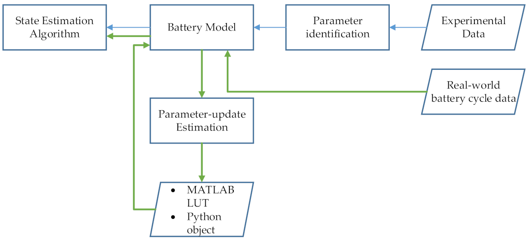
Step 4 of the approach addresses the execution efforts applied on the software segment for implementing a battery DT. The commonly used software and programming languages of battery modeling are MATLAB, COMSOL or Python. Irrespective of the chosen platform, the flowchart of the implementation steps is shown in Figure 3. The green arrows denote the workflow of battery DT while the blue arrows denote that of a battery mode.
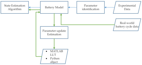
Figure 3.
Software segment for implementation steps.
The conventional steps of building a battery model using experimental inputs for its parameter identification followed by the state estimation is the preliminary implementation step for battery DT. Real-world battery data (i.e., terminal voltage, load current and temperature) is then integrated with the model, which means they are added as time series input by importing the battery data (in .csv or other compatible formats). The parameter-update estimation step can be computationally handled in a dedicated code or in the differential solver tools in MATLAB or Python. A standard method in MATLAB for accessing the parameters is through lookup tables (LUT). For model parameter-update in MATLAB, the parameter (in the required format) is uploaded to the workspace and directly imported to the LUT. Alternatively, in Python, re-assigning or updating an input parameter is relatively easy by direct access and assignment of the parameter in its respective object. Finally, the battery DT is subjected to the state estimation algorithm.
3.5. Step 5: Battery DT KPI Quantification
Lastly, but most importantly, it is necessary to identify the benefits of the battery DT to draw light on its significance for the battery industry. Referring to the problem identified in the Section 1 of the paper that without substantial effort to describe and quantify benefits, it is challenging to suggest that the DT concept itself may be the most appropriate solution to the challenges faced by each particular industry. To support a holistic battery DT implementation in the future, both qualitative and quantitative KPIs are identified and elaborated below:
- Investment
- ◦
- Effect on optimization cost due to battery DT functionalities.
- ◦
- Cost to establish data acquisition from BMS to the battery model. Here, we assume the preexisting cost of sensors installed on the BMS and the cells.
- ◦
- Cost of data storage method, i.e., cloud server, memory drive, etc.
- ◦
- Computational cost of simulating the algorithms of the battery DT.
- Time
- ◦
- Time needed for the state estimation algorithms, optimization algorithms and other battery DT functionalities
- ◦
- Time to retrieve battery data from its application and assign it to the DT
- ◦
- Speed of battery DT alignment with actual battery, i.e., total time for executing the parameter-update step.
- Accuracy
- ◦
- Accuracy of parameter identification.
- ◦
- Accuracy of parameter-update estimation parameter identification.
- ◦
- Accuracy of state estimation
- Functionalities
- ◦
- DT functionalities that support the battery designers (battery design optimization)
- ◦
- DT functionalities that support the battery users
- ◦
- DT functionalities that support the battery EoL handler (RUL assessment)
Note: Functionalities is a qualitative KPI. We determine the services that a DT is capable of providing its users through the battery DT functionalities. The accuracy of those services across the battery lifecycle is a KPI for evaluating the benefits of using a battery DT.
4. Results
Here, we highlight the usage of approach in Section 3. The number and variety of existing open-source battery modeling software packages (MATLAB, COMSOL, DUALFOIL, fastDFN, to name a few) have made it convenient for academics and industrial battery designers to begin with partially developed and functional models rather than building the battery model from scratch.
Utilization of experimental results for estimating the battery model parameters is necessary during initial design of the model. However, for estimating the battery state that is already in use for N cycles, experimental validation of terminal voltage followed by a minimization optimization algorithm is impossible. Here, the alternative is that either the BMS provides the voltage values of each cell through the voltage sensor or the parameter-update is identified through the aging physics of the battery.
PyBaMM (Python Battery Mathematical Modelling) is an open-source Python package that can solve continuum models. It can be coupled with other software packages and is capable of solving standard electrochemical battery models. Documentations for using PyBaMM are available [67,68] and the results show that PyBaMM can facilitate the model parameter-update estimation.
The data structure of battery models in PyBaMM is a collection of symbolic expression trees (variable, parameter, addition, multiplication, and gradient). These enable mathematical representation of the model components. The addition of a new battery model in PyBaMM requires initialization of attributes such as: (1) variable boundary conditions; (2) governing equations; (3) initial conditions; (4) output variables of the model; (5) other optional attributes (geometry, computation solver, parameter values, termination events, and battery region).
PyBaMM provides parameter sets based on experimental data provided in literature [69,70] which are used as the reference parameter values in this paper. Types of parameter for all the components (cells, electrolytes, negative electrode, positive electrode, SEI, separators) includes, macroscale geometry [m] or microstructure, current collector conductivities [S m−1], current collector density [kg m−3], current collector specific heat capacity [J· kg−1 K−1], current collector thermal conductivity [W m−1 K−1], nominal cell capacity [A.h], current function [A], electrode properties, and interfacial reactions.
According to Figure 3, the model is first fed with the charge/discharge cycle data through an excel file. In the following execution, a high acceleration aggressive driving schedule—US06 is used to discharge the DFN model. Code segments (2), (3) and (4) are the cycle integration steps.
Experiment1 = pybamm.Experiment ([“Charge at 1 A until 4.1 V”, “Hold at 4.1 V until 50 mA”])
Experiment2 = pybamm.Experiment([(“Discharge at 1C for 0.5 h”, “Discharge at C/20 for 0.5 h”)] × 2 + [(“Charge at 0.5 C for 45 min”,)]
Experiment3 = pybamm.Experiment([(“Discharge at 2C until 3.3 V”, “Rest for 0.5 h”, “Charge at 1 A until 4.1 V”, “Hold at 4.1 V until 50 mA”)])
The Python program was written based on the provided examples in the documentation, hence the results can be reproduced. PyBaMM operates with respect to a defined set of input parameters (~97) and output variables (~400). The PyBaMM program steps highlight the ease of following the implementation steps of Figure 3. It can be considered the means to develop battery DTs, mainly due to fast access to the model parameters in Python. Further analysis and research with different input data and parameter identification are definitely needed in order to implement a holistic battery DT. The correctness of the findings in these results are dependent on the precision of the PDE and ODE solvers in PyBaMM.
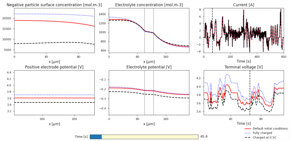
In Figure 4, the default DFN model is assigned with the two types of charging preconditions—(2) and (3). The battery model is fully charged using 2, followed by the final state of the experimental solution being mapped to the initial conditions of the next discharge cycle. Similarly, using (3), the battery model is completely discharged followed by slow charge at 0.5 C for 45 min. Likewise, the final state of the experimental solution is mapped as the initial condition for the consequent discharge cycle. The surface concentration, electrode potentials, and terminal voltage values are compared for the three scenarios, i.e., default battery initial state, fully charged, and slow charged. The comparison implies that the effect of charging under varying conditions can be mirrored to the consequent discharge cycle. This helps in running the state estimation procedures after certain discharge cycles with relevant initial conditions.
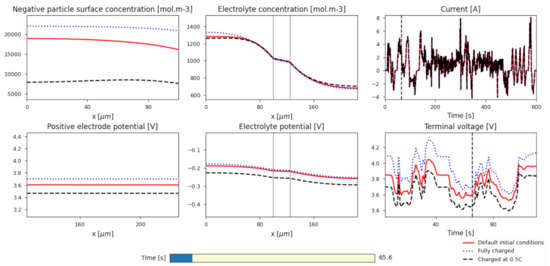
Figure 4.
DFN model discharge results with different preconditions. Fully charged—code statement (2). Complete discharge and slow charge—code statement (3).
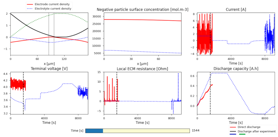
Code segment (4) is a variation of (3), where the model is discharged at 2 C until 3.3 V, followed by 30 min rest and full charge until 4.1 V. Figure 5 and Figure 6 show that a discharge/charge cycle with respect to (4) is followed by the US06 drive cycle. Similar to the processing of Figure 4, the final state of the model at the end of the charge cycle (Experiment 3) is used to update the initial conditions at the beginning of the discharge cycle. Figure 5 compares the model behavior with direct discharge and discharge after the Experiment 3. The plot of terminal voltage reflects that an accurate terminal voltage estimation is possible when the model parameters are appropriately updated with respect to the operation of the actual battery. Figure 6 partially repeats a section of Figure 5. It mainly shows the DFN model output variables for charge and discharge cycle based on code segment (4) and the US06 drive cycle.
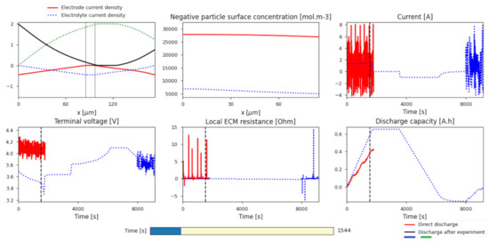
Figure 5.
Comparison between output parameters of two discharge characteristics.
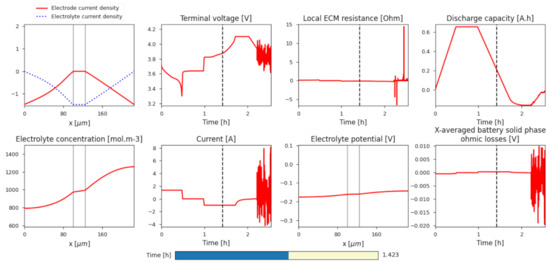
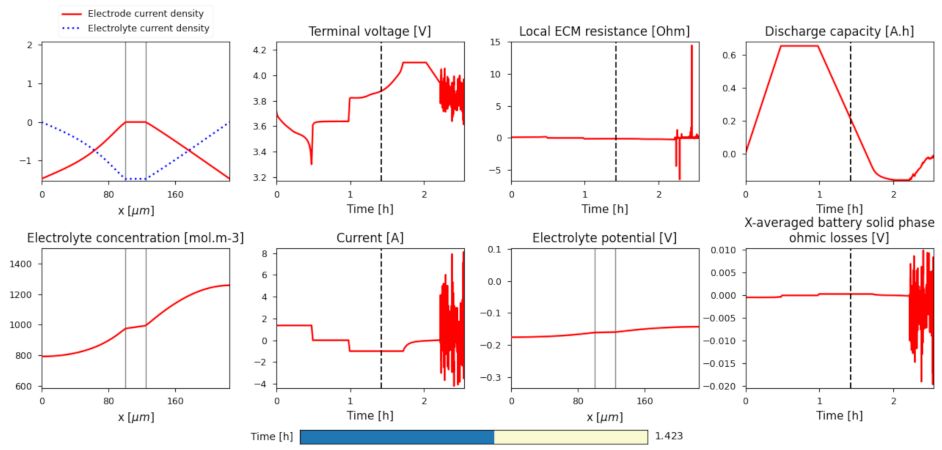
Figure 6.
DFN model output variables for discharge based on code statement—(4).
Some of the variables are two-dimensional, with respect to time and the distance from the anode current collector (x). Thus, the graphs change as time is modified. From Figure 5, the output variables for both the scenarios (i.e., only discharge and charge followed by discharge) are retrieved in MATLAB files in 1D or 2D arrays. The output variable set shown in the following code segment can be used to calculate the degradation mechanisms of the electrode, separator, and electrolyte.
solution.save_data(“Output_AfterDischarging.mat”,
[“Time [h]”, “Current [A]”, “Terminal voltage [V]”, “x [m]”,
“Electrolyte concentration [mol.m-3]”,
“Electrolyte potential [V]”,
“Negative particle surface concentration [mol.m-3]”,
“Negative electrode potential [V]”,
“Positive particle surface concentration [mol.m-3]”,
“Positive electrode potential [V]”,
“Negative electrode surface area to volume ratio [m-1]”,
“Positive electrode surface area to volume ratio [m-1]”,
“Positive electrode active material volume fraction”,
“Negative electrode active material volume fraction”], to format=“matlab”)
Hence, the first parameter-update method of 3.3 is realizable in PyBaMM. This example was based on only a small range of driving schedules, while the input charge/discharge cycles are much longer in reality. There also arises an alternative of a straightforward implementation through continuous concatenation of the driving cycles. While that will work for small durations, a very high computation power will be needed to cycle the model through the complete usage phase using a single concatenated file. The model parameter-update during usage keeps the battery DT up-to-date with the actual cell after every N cycle.
Knowledge of which driving cycle parameters affects the model parameters might not always be computationally practical because evaluating the exact values of each parameter is not practically possible. Model reduction is, therefore, an important component, especially of electrochemical battery models. However, understanding potential dependencies will directly impact the formulation of the estimation algorithms’ objective function and cost functions.
The output files generated from the results contribute to parameter retrieval and comparison, it can further be integrated with existing battery state estimation techniques. The extensive parameter set that the DFN model provides complements the requirements of the high fidelity prediction algorithms that aim for high accuracy, irrespective of the computation costs. Additionally, the output parameter set can be used for generating training data for data-driven predictions in real-time applications.
Due to the unavailability of operational data, the KPIs identified in Step 5 of the approach are not be quantified for this implementation. However, comprehensive testing and KPI quantification will be investigated in future research.
5. Discussion
The following points focus on the unaddressed issues that remain unresolved but are considerably broad in scope to be handled in one paper:
- Level of fidelity expected from a battery DT—A model that captures the electrical, thermal, electrochemical, mechanical and aging aspects of a battery is deemed a high fidelity model. The reality and practicality of such a model are not clear. The cost and time needed for an exhaustive high-fidelity battery DT are high, and the estimate of accuracy improvement is also missing;
- Number of DTs across the battery lifecycle—The idea of a DT across the lifecycle of a product is not entirely understood. This is due to the uncertainty of the number of DTs needed in such cases. Either there is one DT with a large capacity, or there are many small-sized DTs coupled together. For battery DT, the coupling of process and product DT is a possible use case during manufacturing;
- Scaling the battery DT to module and pack-level DT—Achieving battery DTs at scale will require a reduction in technical barriers for their adoption. This implies that for a pack-level battery DT, the number of sensors and the amount of data retrieved will drastically increase. Hence, the data acquisition and storage needs to be seamless;
- Accuracy of behavioral prediction using battery DT—For commercial utilization of battery DTs, it is necessary to compare and quantify the accuracy of existing BMS predictions vs. the prediction of battery DT. Quantification and comparison of percentage error in DT estimations should be the primary focus in future works.
6. Conclusions
An approach for battery DT implementation was presented. The 5-step approach allows the readers to recognize the difference between a battery model and battery DT implementation. The first challenge recognized for battery DT implementation is making the battery operational data available to the model. Cloud services have been integrated with onboard-BMSs in the past, but this is not common. In the coming years, the data integration method for battery DTs has to be standardized, even though it might entail initial investment and implementation time. The second challenge recognized for battery DT implementation is that the method of model parameter-update during usage is not well established and still needs further research. The results of the paper indicate that, if tracked, the DFN model parameters will keep changing after a certain period of usage and cycling. The other methods proposed for parameter-update in the paper will be investigated in future work.
This paper provides a consistent view of a battery DT and the added value, i.e., its functionalities that it offers during battery operation and EoL. The benefits of battery DTs are: improved representation, performance estimation, behavioral predictions, optimization strategies, and integration of battery life cycle attributes to the remaining DT functions. Based on the results provided in this paper, a battery DT can widen the scope of current BMS functionalities by evaluating the degradation effect that the driving cycle has on the battery from an electrochemical or electrical perspective.
The quantitative uncertainty of the potential costs, infrastructure challenges, and return on investments for battery DTs still exist. However, the KPIs identified in this paper will play a significant role in quantifying the battery DT attributes. Promising future scope exists in evaluating the KPIs for DT across the life cycle phases of a battery. As part of the ongoing research to evaluate the feasibility of battery DTs, its functionalities and quantification of its attributes across the lifecycle will be explored in future works.
Author Contributions
Conceptualization, S.S.; approach, S.S.; implementation, S.S.; writing—original draft preparation, S.S.; writing—review and editing, M.W., K.P.B.; visualization, S.S.; project administration, M.W.; funding acquisition, M.W. and K.P.B.; supervision, M.W. and K.P.B. All authors have read and agreed to the published version of the manuscript.
Funding
This research was funded by the Federal Ministry for Economic Affairs and Energy (BMWi), funding code 19I21014C. The authors wish to thank the Federal Ministry for Economic Affairs and Energy, Germany for funding this work as part of the accompanying research of the project “iBMS”.
Institutional Review Board Statement
Not applicable.
Informed Consent Statement
Not applicable.
Data Availability Statement
The data presented in this study are openly available in GitHub at [69].
Conflicts of Interest
The authors declare no conflict of interest.
Appendix A
Table A1.
Governing equations of DFN model along with the phenomenon that describes the diffusion, charge/mass conservation and flux density in DFN model [46,71].
Table A1.
Governing equations of DFN model along with the phenomenon that describes the diffusion, charge/mass conservation and flux density in DFN model [46,71].
| DFN Model | Derived through | Governing Equations 1 |
|---|---|---|
| Solid phase mass transport equation—Li+ concentration in electrodes and separator | Fick’s law of diffusion | |
| Liquid phase mass transport equation—Li+ concentration in electrolyte | Conservation of Li+ ions (Conservation of mass) | |
| Solid phase charge transport equation—Potential in electrode | Ohm’s law (Conservation of charge) | |
| Liquid phase charge transport equation—Potential in electrolyte | Ohm’s law and Kirchhoff’s law (Concentrated solution theory, conservation of charge) | |
| Flux density between solid and liquid phase | Butler-Volmer Equation |
1 Concentration of lithium in the solid phase (x, r, t) and electrolyte (x,t). Electric potential in the solid phase ϕs(x,t) and electrolyte ϕe(x,t). Flux density between solid phase and electrolyte j(x,t). Remaining symbols are described in Table 1.
Table A2.
Equations of ECM model in the time domain for pulse current [72].
Table A2.
Equations of ECM model in the time domain for pulse current [72].
| ECM Model Equations | Variables |
|---|---|
| pi = fi(SOC, SOH, T, I) p1 = {VOCV, R1, C1, RS} | i is the i-th parameter of the model. R1 and C1 are the polarization resistance and capacitance and RS is the ohmic resistance. VOCV is the open circuit voltage |
| Vt = VOCV − V1 − VRs; VRs = I * RS | where VRs refers to the voltage reduction from Rs and Vt is the terminal voltage |
| SOC = SOC0 − | SOC calculation using CC, where C is capacity, Ib is current, and SOC0 is the initial SOC |
References
- Singh, S.; Weeber, M.; Birke, K.-P. Advancing digital twin implementation: A toolbox for modelling and simulation. Procedia CIRP 2021, 99, 567–572. [Google Scholar] [CrossRef]
- Shafto, M.; Conroy, M.; Doyle, R.; Glaessgen, E.; Kemp, C.; LeMoigne, J.; Wang, L. Modeling, simulation, information technology & processing roadmap. Natl. Aeronaut. Space Adm. 2012, 32, 1–38. [Google Scholar]
- Boschert, S.; Rosen, R. Digital twin—The simulation aspect. In Mechatronic Futures; Springer: Cham, Switzerland, 2016; pp. 59–74. [Google Scholar]
- Kunath, M.; Winkler, H. Integrating the Digital Twin of the manufacturing system into a decision support system for improving the order management process. Procedia CIRP 2018, 72, 225–231. [Google Scholar] [CrossRef]
- Batty, M. Digital twins. Environ. Plan. B Urban. Anal. City Sci. 2018, 45, 817–820. [Google Scholar] [CrossRef]
- Wright, L.; Davidson, S. How to tell the difference between a model and a digital twin. Adv. Model. Simul. Eng. Sci. 2020, 7, 13. [Google Scholar] [CrossRef]
- Arup Research. Digital Twin—Towards a Meaningful Framework. Available online: https://research.arup.com/publications/digital-twin-towards-a-meaningful-framework/ (accessed on 26 July 2021).
- Singh, M.; Fuenmayor, E.; Hinchy, E.P.; Qiao, Y.; Murray, N.; Devine, D. Digital Twin: Origin to Future. ASI 2021, 4, 36. [Google Scholar] [CrossRef]
- Saracco, R. Digital Twins: Bridging Physical Space and Cyberspace. Computer 2019, 52, 58–64. [Google Scholar] [CrossRef]
- Al-Ali, A.R.; Gupta, R.; Zaman Batool, T.; Landolsi, T.; Aloul, F.; Al Nabulsi, A. Digital twin conceptual model within the context of internet of things. Future Internet 2020, 12, 163. [Google Scholar] [CrossRef]
- Lin, W.D.; Low, M.Y.H. Concept design of a system architecture for a manufacturing cyber-physical Digital Twin system. In Proceedings of the 2020 IEEE International Conference on Industrial Engineering and Engineering Management (IEEM), Singapore, 14–17 December 2020; IEEE: Piscataway, NJ, USA, 2020; pp. 1320–1324, ISBN 978-1-5386-7220-4. [Google Scholar]
- Wagg, D.J.; Worden, K.; Barthorpe, R.J.; Gardner, P. Digital Twins: State-of-the-Art and Future Directions for Modeling and Simulation in Engineering Dynamics Applications. ASCE-ASME J. Risk. Uncert. Eng. Syst. Part. B Mech. Eng. 2020, 6, 101001. [Google Scholar] [CrossRef]
- Lim, K.Y.H.; Zheng, P.; Chen, C.-H. A state-of-the-art survey of Digital Twin: Techniques, engineering product lifecycle management and business innovation perspectives. J. Intell. Manuf. 2020, 31, 1313–1337. [Google Scholar] [CrossRef]
- Jones, D.; Snider, C.; Nassehi, A.; Yon, J.; Hicks, B. Characterising the Digital Twin: A systematic literature review. CIRP J. Manuf. Sci. Technol. 2020, 29, 36–52. [Google Scholar] [CrossRef]
- Merkle, L.; Segura, A.S.; Grummel, J.T.; Lienkamp, M. Architecture of a digital twin for enabling digital services for battery systems. In Proceedings of the 2019 IEEE International Conference on Industrial Cyber Physical Systems (ICPS), Taipei, Taiwan, 6–9 May 2019; IEEE: Piscataway, NJ, USA, 2019; pp. 155–160. [Google Scholar]
- Schluse, M.; Atorf, L.; Rossmann, J. Experimentable digital twins for model-based systems engineering and simulation-based development. In Proceedings of the 2017 Annual IEEE International Systems Conference (SysCon), Montreal, QC, Canada, 24–27 April 2017; IEEE: Piscataway, NJ, USA, 2017. ISBN 9781509046232. [Google Scholar]
- Josifovska, K.; Yigitbas, E.; Engels, G. Reference Framework for Digital Twins within cyber-physical systems. In Proceedings of the 2019 IEEE/ACM 5th International Workshop on Software Engineering for Smart Cyber-Physical Systems (SEsCPS), Montreal, QC, Canada, 28 May 2019; IEEE: Piscataway, NJ, USA, 2019; pp. 25–31, ISBN 978-1-7281-2282-3. [Google Scholar]
- Kritzinger, W.; Karner, M.; Traar, G.; Henjes, J.; Sihn, W. Digital Twin in manufacturing: A categorical literature review and classification. IFAC-Pap. 2018, 51, 1016–1022. [Google Scholar] [CrossRef]
- Sitterly, M.; Le Wang, Y.; Yin, G.G.; Wang, C. Enhanced identification of battery models for real-time battery management. IEEE Trans. Sustain. Energy 2011, 2, 300–308. [Google Scholar] [CrossRef]
- Niederer, S.A.; Sacks, M.S.; Girolami, M.; Willcox, K. Scaling digital twins from the artisanal to the industrial. Nat. Comput. Sci. 2021, 1, 313–320. [Google Scholar] [CrossRef]
- Qu, X.; Song, Y.; Liu, D.; Cui, X.; Peng, Y. Lithium-ion battery performance degradation evaluation in dynamic operating conditions based on a digital twin model. Microelectron. Reliab. 2020, 114, 113857. [Google Scholar] [CrossRef]
- Li, W.; Rentemeister, M.; Badeda, J.; Jöst, D.; Schulte, D.; Sauer, D.U. Digital twin for battery systems: Cloud battery management system with online state-of-charge and state-of-health estimation. J. Energy Storage 2020, 30, 101557. [Google Scholar] [CrossRef]
- Merkle, L.; Pöthig, M.; Schmid, F. Estimate e-Golf Battery State Using Diagnostic Data and a Digital Twin. Batteries 2021, 7, 15. [Google Scholar] [CrossRef]
- Peng, Y.; Zhang, X.; Song, Y.; Liu, D. A low cost flexible digital twin platform for spacecraft lithium-ion battery pack degradation assessment. In Proceedings of the 2019 IEEE International Instrumentation and Measurement Technology Conference (I2MTC), Auckland, New Zealand, 20–23 May 2019; IEEE: Piscataway, NJ, USA, 2019; pp. 1–6, ISBN 978-1-5386-3460-8. [Google Scholar]
- Baumann, M.; Rohr, S.; Lienkamp, M. Cloud-connected battery management for decision making on second-life of electric vehicle batteries. In Proceedings of the 2018 Thirteenth International Conference on Ecological Vehicles and Renewable Energies (EVER), Monte-Carlo, Monaco, 10–12 April 2018; IEEE: Piscataway, NJ, USA, 2018; pp. 1–6, ISBN 978-1-5386-5966-3. [Google Scholar]
- Ramachandran, R.; Ganeshaperumal, D.; Subathra, B. Parameter estimation of battery pack in EV using extended kalman filters. In Proceedings of the 2019 IEEE International Conference on Clean Energy and Energy Efficient Electronics Circuit for Sustainable Development (INCCES), Krishnankoil, India, 18–20 December 2019; IEEE: Piscataway, NJ, USA, 2019; pp. 1–5, ISBN 978-1-7281-4407-8. [Google Scholar]
- Wu, B.; Widanage, W.D.; Yang, S.; Liu, X. Battery digital twins: Perspectives on the fusion of models, data and artificial intelligence for smart battery management systems. Energy AI 2020, 1, 100016. [Google Scholar] [CrossRef]
- Sancarlos, A.; Cameron, M.; Abel, A.; Cueto, E.; Duval, J.-L.; Chinesta, F. From ROM of electrochemistry to ai-based battery digital and hybrid twin. Arch. Comput. Methods Eng. 2021, 28, 979–1015. [Google Scholar] [CrossRef]
- Soleymani, A.; Maltz, W. Real time prediction of Li-Ion battery pack temperatures in EV vehicles. In Proceedings of the ASME 2020 International Technical Conference and Exhibition on Packaging and Integration of Electronic and Photonic Microsystems, Virtual, 27–29 October 2020; American Society of Mechanical Engineers: New York, NY, USA, 2020; p. 10272020, ISBN 978-0-7918-8404-1. [Google Scholar]
- Ahmed, R.; Gazzarri, J.; Onori, S.; Habibi, S.; Jackey, R.; Rzemien, K.; Tjong, J.; LeSage, J. Model-Based Parameter Identification of Healthy and Aged Li-ion Batteries for Electric Vehicle Applications. SAE Int. J. Alt. Power. 2015, 4, 233–247. [Google Scholar] [CrossRef] [Green Version]
- Dühnen, S.; Betz, J.; Kolek, M.; Schmuch, R.; Winter, M.; Placke, T. Toward green battery cells: Perspective on materials and technologies. Small Methods 2020, 4, 2000039. [Google Scholar] [CrossRef]
- Wang, W.; Wang, J.; Tian, J.; Lu, J.; Xiong, R. Application of Digital Twin in Smart Battery Management Systems. Chin. J. Mech. Eng. 2021, 34, 1–19. [Google Scholar] [CrossRef]
- Balasingam, B.; Ahmed, M.; Pattipati, K. Battery Management Systems—Challenges and Some Solutions. Energies 2020, 13, 2825. [Google Scholar] [CrossRef]
- Gabbar, H.A.; Othman, A.M.; Abdussami, M.R. Review of Battery Management Systems (BMS) Development and Industrial Standards. Technologies 2021, 9, 28. [Google Scholar] [CrossRef]
- Lin, Q.; Wang, J.; Xiong, R.; Shen, W.; He, H. Towards a smarter battery management system: A critical review on optimal charging methods of lithium ion batteries. Energy 2019, 183, 220–234. [Google Scholar] [CrossRef]
- Orion BMS 2. Orion Li-Ion Battery Management System. Available online: https://www.orionbms.com/products/orion-bms-standard/ (accessed on 27 July 2021).
- LION Smart. LION Smart—Battery Management System (BMS). Available online: https://lionsmart.com/en/battery-management-system/ (accessed on 27 July 2021).
- van Dao, Q.; Dinh, M.-C.; Kim, C.S.; Park, M.; Doh, C.-H.; Bae, J.H.; Lee, M.-K.; Liu, J.; Bai, Z. Design of an effective State of Charge estimation method for a lithium-ion battery pack using extended kalman filter and artificial neural network. Energies 2021, 14, 2634. [Google Scholar] [CrossRef]
- Danko, M.; Adamec, J.; Taraba, M.; Drgona, P. Overview of batteries State of Charge estimation methods. Transp. Res. Procedia 2019, 40, 186–192. [Google Scholar] [CrossRef]
- Rivera-Barrera, J.; Muñoz-Galeano, N.; Sarmiento-Maldonado, H. SoC Estimation for Lithium-ion Batteries: Review and Future Challenges. Electronics 2017, 6, 102. [Google Scholar] [CrossRef] [Green Version]
- Wang, Y.; Tian, J.; Sun, Z.; Wang, L.; Xu, R.; Li, M.; Chen, Z. A comprehensive review of battery modeling and state estimation approaches for advanced battery management systems. Renew. Sustain. Energy Rev. 2020, 131, 110015. [Google Scholar] [CrossRef]
- Meng, J.; Luo, G.; Ricco, M.; Swierczynski, M.; Stroe, D.-I.; Teodorescu, R. Overview of lithium-ion battery modeling methods for State-of-Charge estimation in electrical vehicles. Appl. Sci. 2018, 8, 659. [Google Scholar] [CrossRef] [Green Version]
- Schellenberg, S.; Berndt, R.; Eckhoff, D.; German, R. A Computationally inexpensive battery model for the microscopic simulation of electric vehicles. In Proceedings of the 2014 IEEE 80th Vehicular Technology Conference (VTC Fall), Vancouver, BC, Canada, 14–17 September 2014; IEEE: Piscataway, NJ, USA, 2014; pp. 1–6, ISBN 978-1-4799-4449-1. [Google Scholar]
- Li, Y.; Vilathgamuwa, D.M.; Farrell, T.W.; Choi, S.S.; Tran, N.T. An equivalent circuit model of li-ion battery based on electrochemical principles used in grid-connected energy storage applications. In Proceedings of the 2017 IEEE 3rd International Future Energy Electronics Conference and ECCE Asia (IFEEC 2017—ECCE Asia), Kaohsiung, Taiwan, 3–7 June 2017; IEEE: Piscataway, NJ, USA, 2017; pp. 959–964, ISBN 978-1-5090-5157-1. [Google Scholar]
- Kim, H.-K.; Lee, K.-J. Scale-Up of Physics-Based Models for Predicting Degradation of Large Lithium Ion Batteries. Sustainability 2020, 12, 8544. [Google Scholar] [CrossRef]
- Jokar, A.; Rajabloo, B.; Désilets, M.; Lacroix, M. Review of simplified Pseudo-two-Dimensional models of lithium-ion batteries. J. Power Sources 2016, 327, 44–55. [Google Scholar] [CrossRef]
- Barcellona, S.; Piegari, L. Lithium Ion Battery Models and Parameter Identification Techniques. Energies 2017, 10, 2007. [Google Scholar] [CrossRef] [Green Version]
- Uddin, K.; Perera, S.; Widanage, W.; Somerville, L.; Marco, J. Characterising Lithium-Ion Battery Degradation through the Identification and Tracking of Electrochemical Battery Model Parameters. Batteries 2016, 2, 13. [Google Scholar] [CrossRef]
- Forman, J.C.; Moura, S.J.; Stein, J.L.; Fathy, H.K. Genetic parameter identification of the Doyle-Fuller-Newman model from experimental cycling of a LFP battery. In Proceedings of the 2011 American Control Conference, San Francisco, CA, USA, 29 June–1 July 2011; IEEE: Piscataway, NJ, USA, 2011; pp. 362–369, ISBN 978-1-4577-0081-1. [Google Scholar]
- Rahman, M.A.; Anwar, S.; Izadian, A. Electrochemical model parameter identification of a lithium-ion battery using particle swarm optimization method. J. Power Sources 2016, 307, 86–97. [Google Scholar] [CrossRef]
- Yang, G. Battery parameterisation based on differential evolution via a boundary evolution strategy. J. Power Sources 2014, 245, 583–593. [Google Scholar] [CrossRef]
- Yang, K.; Tang, Y.; Zhang, Z. Parameter Identification and State-of-Charge Estimation for Lithium-Ion Batteries Using Separated Time Scales and Extended Kalman Filter. Energies 2021, 14, 1054. [Google Scholar] [CrossRef]
- Harlow, J.E.; Ma, X.; Li, J.; Logan, E.; Liu, Y.; Zhang, N.; Ma, L.; Glazier, S.L.; Cormier, M.M.E.; Genovese, M.; et al. A Wide Range of Testing Results on an Excellent Lithium-Ion Cell Chemistry to be used as Benchmarks for New Battery Technologies. J. Electrochem. Soc. 2019, 166, A3031–A3044. [Google Scholar] [CrossRef]
- Jin, N.; Danilov, D.L.; van den Hof, P.M.; Donkers, M. Parameter estimation of an electrochemistry-based lithium-ion battery model using a two-step procedure and a parameter sensitivity analysis. Int. J. Energy Res. 2018, 42, 2417–2430. [Google Scholar] [CrossRef]
- Li, W.; Cao, D.; Jöst, D.; Ringbeck, F.; Kuipers, M.; Frie, F.; Sauer, D.U. Parameter sensitivity analysis of electrochemical model-based battery management systems for lithium-ion batteries. Appl. Energy 2020, 269, 115104. [Google Scholar] [CrossRef]
- Miniguano, H.; Barrado, A.; Lazaro, A.; Zumel, P.; Fernandez, C. General Parameter Identification Procedure and Comparative Study of Li-Ion Battery Models. IEEE Trans. Veh. Technol. 2020, 69, 235–245. [Google Scholar] [CrossRef]
- Madani, S.; Schaltz, E.; Knudsen Kær, S. Effect of Current Rate and Prior Cycling on the Coulombic Efficiency of a Lithium-Ion Battery. Batteries 2019, 5, 57. [Google Scholar] [CrossRef] [Green Version]
- Tran, M.-K.; Mevawala, A.; Panchal, S.; Raahemifar, K.; Fowler, M.; Fraser, R. Effect of integrating the hysteresis component to the equivalent circuit model of Lithium-ion battery for dynamic and non-dynamic applications. J. Energy Storage 2020, 32, 101785. [Google Scholar] [CrossRef]
- Ovejas, V.J.; Cuadras, A. Effects of cycling on lithium-ion battery hysteresis and overvoltage. Sci. Rep. 2019, 9, 14875. [Google Scholar] [CrossRef]
- Severson, K.A.; Attia, P.M.; Jin, N.; Perkins, N.; Jiang, B.; Yang, Z.; Chen, M.H.; Aykol, M.; Herring, P.K.; Fraggedakis, D.; et al. Data-driven prediction of battery cycle life before capacity degradation. Nat. Energy 2019, 4, 383–391. [Google Scholar] [CrossRef] [Green Version]
- Stroe, A.-I.; Knap, V.; Stroe, D.-I. Comparison of lithium-ion battery performance at beginning-of-life and end-of-life. Microelectron. Reliab. 2018, 88–90, 1251–1255. [Google Scholar] [CrossRef]
- Atalay, S.; Sheikh, M.; Mariani, A.; Merla, Y.; Bower, E.; Widanage, W.D. Theory of battery ageing in a lithium-ion battery: Capacity fade, nonlinear ageing and lifetime prediction. J. Power Sources 2020, 478, 229026. [Google Scholar] [CrossRef]
- Boovaragavan, V.; Harinipriya, S.; Subramanian, V.R. Towards real-time (milliseconds) parameter estimation of lithium-ion batteries using reformulated physics-based models. J. Power Sources 2008, 183, 361–365. [Google Scholar] [CrossRef]
- Ali, M.; Kamran, M.A.; Kumar, P.S.; Himanshu; Nengroo, S.H.; Khan, M.A.; Hussain, A.; Kim, H.-J. An Online Data-Driven Model Identification and Adaptive State of Charge Estimation Approach for Lithium-ion-Batteries Using the Lagrange Multiplier Method. Energies 2018, 11, 2940. [Google Scholar] [CrossRef] [Green Version]
- Hou, Y.; Zhang, Z.; Liu, P.; Song, C.; Wang, Z. Research on a novel data-driven aging estimation method for battery systems in real-world electric vehicles. Adv. Mech. Eng. 2021, 13, 168781402110277. [Google Scholar] [CrossRef]
- Hashemi, S.R. An Intelligent Battery Managment System for Electric and Hybrid Electric Aircraft. Ph.D. Thesis, University of Akron, Akron, OH, USA, 2021. [Google Scholar]
- Sulzer, V.; Marquis, S.G.; Timms, R.; Robinson, M.; Chapman, S.J. Python Battery Mathematical Modelling (PyBaMM). J. Open Res. Softw. 2020, 9, 14. [Google Scholar] [CrossRef]
- Welcome to PyBaMM’s Documentation!—PyBaMM 0.4.0 Documentation. Available online: https://pybamm.readthedocs.io/en/latest/ (accessed on 28 July 2021).
- GitHub. PyBaMM/pybamm/input/parameters/lithium_ion/cells at developpybamm-team/PyBaMM. Available online: https://github.com/pybamm-team/PyBaMM/tree/develop/pybamm/input/parameters/lithium_ion/cells (accessed on 27 July 2021).
- Chen, C.-H.; Brosa Planella, F.; O’Regan, K.; Gastol, D.; Widanage, W.D.; Kendrick, E. Development of Experimental Techniques for Parameterization of Multi-scale Lithium-ion Battery Models. J. Electrochem. Soc. 2020, 167, 80534. [Google Scholar] [CrossRef]
- Luder, D.; Caliandro, P.; Vezzini, A. Enhanced physics-based models for state estimation of Li-Ion batteries. In Proceedings of the Comsol Conference 2020 Europe, Virtual, 14–15 October 2020. [Google Scholar]
- Madani, S.; Schaltz, E.; Knudsen Kær, S. An Electrical Equivalent Circuit Model of a Lithium Titanate Oxide Battery. Batteries 2019, 5, 31. [Google Scholar] [CrossRef] [Green Version]


Publisher’s Note: MDPI stays neutral with regard to jurisdictional claims in published maps and institutional affiliations. |
© 2021 by the authors. Licensee MDPI, Basel, Switzerland. This article is an open access article distributed under the terms and conditions of the Creative Commons Attribution (CC BY) license (https://creativecommons.org/licenses/by/4.0/).