1. Introduction
A Design of Experiments (DoE) is a fascinating and incredibly useful tool to strengthen any study dealing with varying parameters by giving weight to all observations and trends with a minimal number of experiments to run. It allows to look at factors’ individual and combined impacts as well as to optimize inputs for maximum performance. This paper is a methodological publication and conclusions on the case study will be reported in another manuscript for concision reasons.
Although known since the mid-1930s and widely used in the industry, DoE are not often taken into consideration in academia [
1,
2,
3,
4]. This is likely because they could appear intimidating and overwhelming without the right tools and knowledge of mathematics and statistics. In recent years, many software solutions appeared that can remove most of that burden from the user. Unfortunately, with too much automation in a “black box” process, there is always a risk of reaching false positive results without significant meaning. The purpose of this publication is to provide the battery community with a starting point on how to approach DoE with confidence and without the need for advance statistical knowledge. Each step and parameter to draw robust and trustworthy empirical models will be carefully explained and discussed in this work. This publication will only cover the example of a DoE preparation and execution for the formulation of Li-ion battery electrodes, but the overall approach will remain true for other types of DoE or with different materials [
5,
6,
7,
8,
9].
Li-ion battery electrodes are composed of several materials and their respective formulation and content will drastically affect the battery’s performance. Although Li-ion batteries were first commercialized 30 years ago, there is still no consensus on the definitive formulation for a high-power, high-energy, long cycle life electrode. In other words, no single model links a battery’s capacity or energy to its different properties and formulation. Therefore, while investigating new materials, it is necessary to re-test a lot of possible combinations where numerous parameters can have an impact. However, there is no guarantee the knowledge acquired through known systems will be relevant to the next one.
A variety of strategies may be adopted to address this issue, such as browsing all possible factor combinations across their entire range or changing one factor at a time while keeping the others constant. While the former would provide a full understanding of each factor’s impact, it would most likely be impractical due to the very high number of required experiments. For its part, the latter strategy would only require a limited number of experiments; however, it would also limit understanding by preventing the observation of combined interactions, i.e., factors inhibiting or exacerbating each other. A good compromise between these two strategies is a Design of Experiments (DoE). This methodology provides a statistical understanding of the observed process through the creation of an empirical model, which is obtained by running an optimized set of experiments to identify factor impacts and combined interactions.
In the lithium battery research community, this method was previously used to predict the cycle life [
2,
8,
10], for model parameterization [
9,
11], and to analyze the impact of different duty cycles on the degradation of commercial cells [
12]. However, to the best of our knowledge, this method has never been reported for electrode formulation in open literature. The intent of this paper is not to present the full DoE analysis, which will be done in a subsequent publication, but rather to take a unique opportunity to describe the methodology in detail. Explaining the essential aspects of a DoE is often difficult in a full research paper as much focus needs to be on results and discussion.
2. Methodology Description
There are different types of DoE, with a variety of focuses and applications [
1,
4,
5,
6,
7,
13]. In this paper, focus was set on a complex mixture design, illustrated by the formulation of a Li-ion composite electrode. This design is relevant in cases when the study focuses on the properties of a blend where the levels of each factor
xn are interdependent with:
An Optimal Combined Design (OCD) is based on a mixture design with the added complexity of categoric and numeric factors coupled with the mixture factors. A categoric factor, such as the nature of the binder, has discrete levels, while a numeric factor, such as porosity or temperature, has continuous levels but is not a component of the mixture.
The objective of an OCD is to describe a response (
Y) as a function of different factors, by using an empirical model such as the one presented in Equation (2):
In Equation (2),
xn represent the
n design factors, while
a,
b,
c etc., are the coefficients describing the significance of each factor. For example, in the case of Li-ion batteries,
Y might be the maximum available capacity, i.e., the amount of lithium that the electrode is capable of storing. This response may not only be dependent on mixture factors such as the quantity of active material, conductive carbons, and binder, but also numeric factors such as the porosity, and categoric factors such as binder type. Each level of a categoric factor could have different values for coefficients
a,
b,
c, etc., if it was found to have a more significant impact on the response than noise. In this example, two different binders were investigated; therefore, two sets of coefficients will be calculated, each describing the relation of
Y with regard to the mixture components and porosity when the electrode is bound by either of the two binders. All factors will be detailed in
Section 2.3.
Although the planning of a DoE is closely linked to the system under study, the methodology described in this paper is adaptable to other designs. This paper illustrates the setup of an OCD designed to understand the effect of formulation on the capacity of Li-ion batteries at high currents. The mathematics on which the DoE are based will not be discussed here, as there are already numerous resources on this topic [
5,
6,
7]. As these calculations are complex, software assistance in the planning and analysis of the design is highly recommended. Here, Design Expert (Stat-Ease Inc.) was used as a data analytics tool, in conjunction with Matlab (Mathworks) to store and manipulate experimental data.
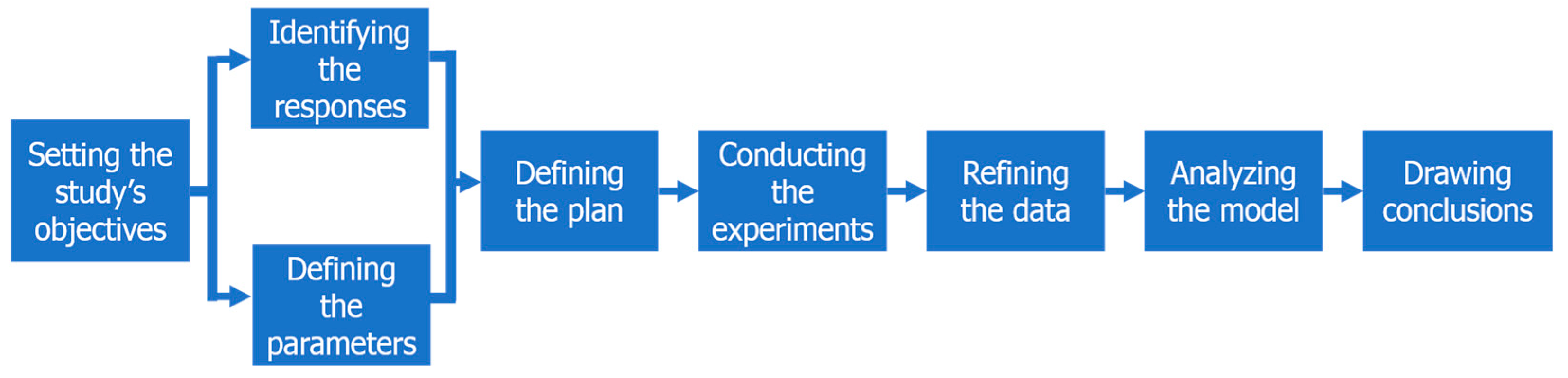
Standard DoE studies are typically articulated around seven or fewer steps [
3,
5,
6,
7]. For the purposes of this study, an eighth step—refining the data—was added, because experimental data is frequently not normally distributed, which in turn prevents the drawing of empirical models. As detailed in
Figure 1, this adapted workflow will serve as an outline for this study.
2.1. Setting the Study’s Objectives
Identifying the weaknesses in a process or phenomenon is the first step in planning a DoE. Designs of Experiments may uncover the relative influence of factors to set up or calibrate a new, unknown or non-optimized process. Plans can also be used to explore new methods or materials linked to the process. In our study of electrode formulation, the incentives were (1) to trial a new binder, and (2) to evaluate the importance of conductive additives for high-power applications. With regard to (1), our previous work [
14] showed promising properties for an elastomer, as compared to polyvinylidene fluoride (PVDF), the most widely used binder in both industry and academia. As these comparisons were based on one formulation only, extension to a much wider formulation range was necessary.
With regard to (2), one of the active material chosen in our study, Li
4Ti
5O
12 (LTO), is a known poor electron conductor [
15], so conductive additives were added to the formulation. Two different morphologies were selected: carbon black (CB) as 50-nm large beads and carbon nanofibers (CNF) as 50-nm-wide and 50- to 250-µm-long cylinders. The former would help electronically connect two neighboring active material particles, while the latter would provide a minimal resistance pathway for electrons across long distances, laterally or transversally from the top to the bottom of the electrode.
2.2. Identifying the Responses
Next, the physical values relevant to the study, i.e., the properties to be optimized, must be identified. These responses should be quantifiable by continuous values and measurable with appreciable precision, since the resulting empirical model will always be, at best, as precise as the measurements on which it is built. In this electrode formulation study, the electrode’s capacity when working under high currents was a response of interest and could be accurately assessed by galvanostatic cycling with potential limitation [
16,
17].
Other responses could have proven to be more complex to both assess and input into a DoE. For example, the rheologic behavior of the slurry could not be a numeric parameter depending on whether the fluid is Newtonian, shear-thinning or shear-thickening [
18].
2.3. Defining the Parameters
Once the responses under study have been identified, a list of all possible factors that can influence the process must be prepared. These factors can be numerous, and a prior understanding of the process should help reduce and classify them as either potential design factors or nuisance factors. Typically, a literature research is a good starting point to garner a broad knowledge of these crucial factors. Complexity, cost, and time should also be considered as the number of experiments required by the Design can rapidly grow given the number of design factors (mixture components, numeric or categoric factors).
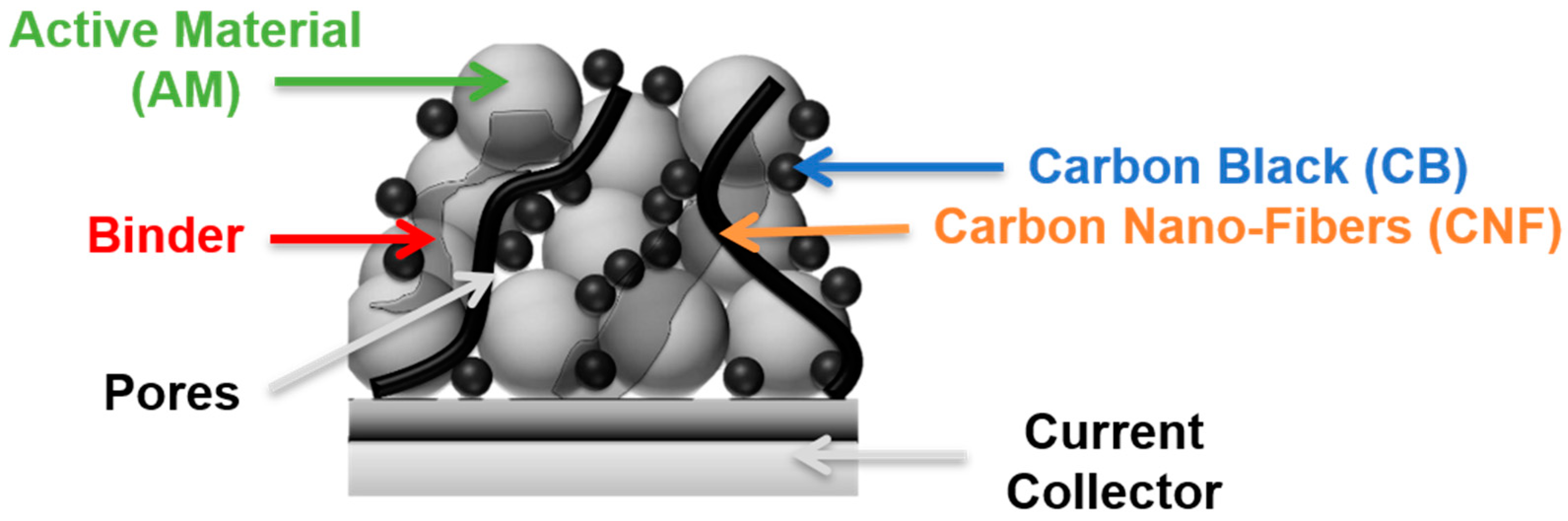
In this work, we chose to study the influence of formulation on select electrodes’ properties with a maximum of four different constituents: one active material, one binder, and two conductive additives. The first is an electrochemically active material such as lithium iron phosphate (LiFePO4) or lithium titanium oxide (Li4Ti5O12) responsible for the storage and release of Li+ ions. The second acts as a binder to provide mechanical cohesion of the active material in the electrode (e.g., a polymer such as polyvinylidene fluoride (PVDF)). If the active material is a poor electron conductor, it is often necessary to add at least one conductive additive (e.g., carbon black, carbon nanofibers, or a conductive polymer) to provide pathways for electrons to compensate for the net charge in the active material under Li+ intercalation or deintercalation. These four components became our design factors. Moreover, since the objective was also to trial a new binder, a categoric factor was added, with two levels to account for the two different binders.
The composite is deposited onto a metallic foil such as aluminum or copper, which is used as a current collector to add mechanical cohesion and provide high electron conductivity between the external circuit and the electrode. Finally, the free volume between the particles, also known as porosity, enables the liquid electrolyte to wet the electrode, and provides pathways for the Li
+ ions in the electrolyte through the electrode,
Figure 2.
The next step was to define the boundaries within which each factor might vary. While a factor’s range has no effect on the number of required experiments to run, it is generally known that the wider the range, the less precise the model will be. Extensive literature is available on Li-ion battery electrodes; although optimal formulations are not known, the constraints inherent to the system are [
19,
20,
21]. On one hand, the active material is the only component responsible for energy storage, so it is highly desirable to maximize its content. On the other hand, the binder is an electronic and ionic insulator. Therefore, its content should be minimized so as not to hinder charge transfers to and from the active material [
22].
Finally, the carbon content should be high enough to ensure sufficient electronic conductivity and hinder any polarization within the electrode while in use under high currents. However, its weight fraction (in %
w)—like the binder—should be kept as small as possible, as it is inactive towards energy storage. Different electronic percolation thresholds (defined as the minimum amount of conductive additives necessary to reach the maximum possible electronic conductivity) have been reported in the literature [
23,
24,
25].
Given these constraints, along with the objective to design a commercially viable high-power battery, the resulting formulation factors defined the design space as follows:
75 to 95%w active material (AM)
0 to 20%w carbon black (CB)
0 to 10%w carbon nanofibers (CNF)
to 20%w binder (B)
For the conductive additives (CA) and binder content, wider ranges than necessary were chosen to identify the optimum percolation threshold and to verify the assumptions on the binder’s insulating nature, respectively.
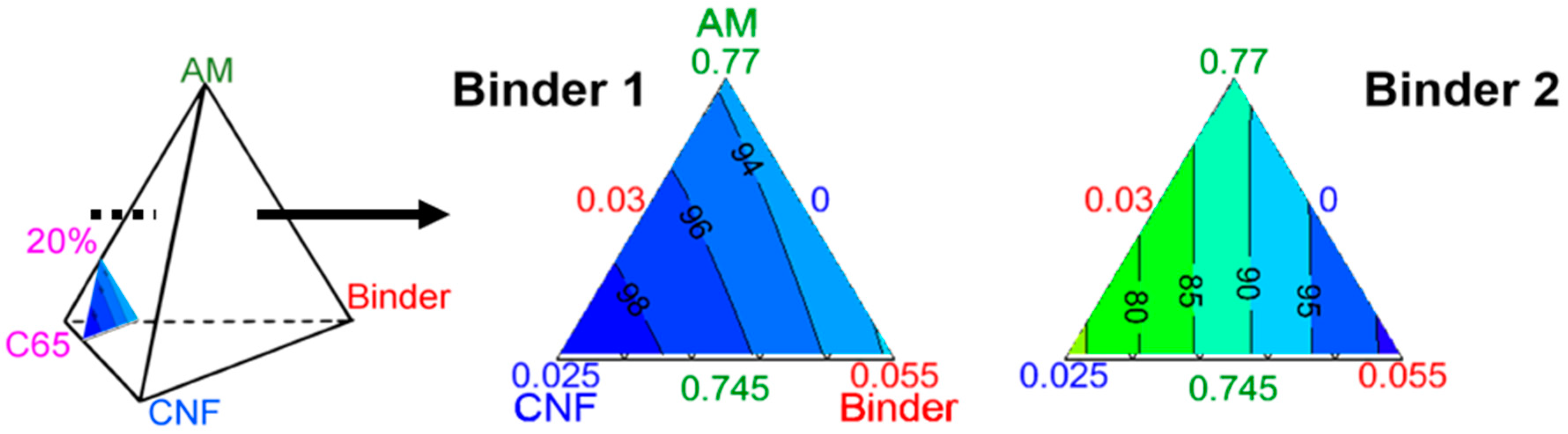
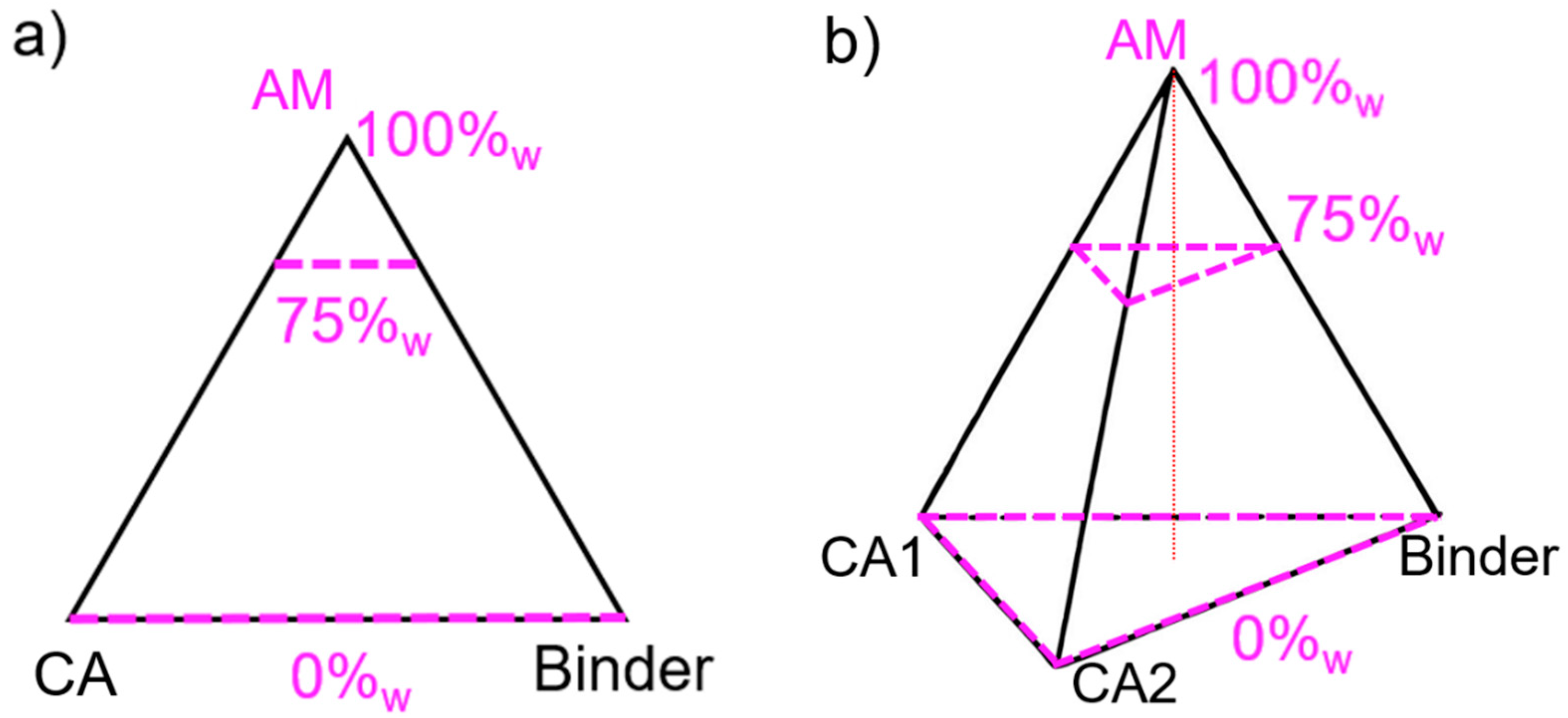
In a three-component plan, the design space comprising all possible mixtures can be represented in a plane as an equilateral triangle. The maximum of each component, e.g., AM, CA and binder, is located at each summit, and the minimum is on the opposite edge, as illustrated in
Figure 3a. For a four-component mixture, another dimension must be added to obtain a regular tetrahedron, where the minimum value for one factor lies on the opposite face to its respective vertex. For any point not situated on the opposite face, the content value is given at the orthogonal projection of the point onto the height.
In the example shown in
Figure 3b, all mixtures on the plane delimited by the top dashed triangle have an AM content of 75%
w and a variety of CB, CNF, and binder content. For this study, and given the set boundaries, the actual design space is only comprised in the upper tetrahedron defined between 100 and 75%
w AM. This design space will be zoomed into and represented as a full tetrahedron in the ensuing discussion.
Other potential design factors, with varying complexity to control and of varying interest to the experimenter, are known to impact the final product. In this example, the active material loading (in mg⋅cm
−2), the porosity, and the thickness of the electrode could be examples of interdependent potential design factors. A thicker electrode, i.e., an electrode with a higher loading, will have a higher ionic and electronic resistance due to longer electronic and ionic pathways [
25,
26]. Thus, at high currents the voltage cut-off would be reached before the battery is fully charged. The porosity is also directly linked to the thickness and formulation of the electrode [
27,
28]. Because the OCD varied the proportion of active material among all experiments, it was impossible to set distinct targets for loading, thickness, and porosity. To ensure experiments were comparable, and for practical reasons, the active material loading was kept constant, in the 4 to 4.5 mg⋅cm
−2 range, and the thickness was allowed to vary. The porosity was then held constant in the 40 to 50%
v range. This approach helps to guarantee that the variations in observed responses were due to variations in formulation only.
The final factors to consider were nuisance and noise. Nuisance factors are difficult to control and yet may have a non-negligible impact on the process. Some of these factors, like slurry rheology, are moderately controllable while others, such as ambient hygrometry or temperature, are uncontrollable on a lab scale. These factors were accounted for when analyzing the responses’ residuals (the difference between observed and predicted values). For their part, noise factors such as experimenter bias were mitigated by randomizing the experiments.
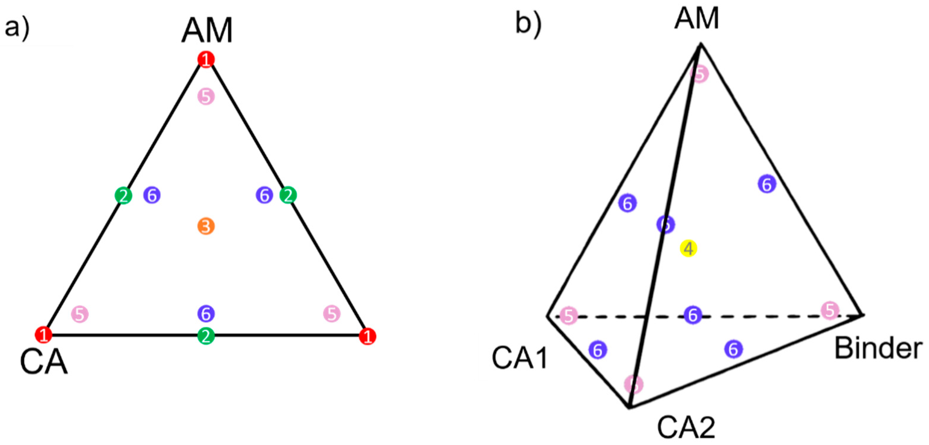
2.4. Defining the Plan
With the design space defined, the next step was to select the experiments (=mixtures) that would best encompass it. Some excellent choices include mixtures situated at (1) the summits, (2) the center of edges, (3) the center of faces, and, if applicable, (4) the center of the tetrahedron (see
Figure 4). Except for the latter, these points force at least one component to 0%
w, and therefore (5) axial check blends and (6) interior check blends are also recommended. To keep
Figure 4b easily readable, points (1) to (3) were not displayed, but can be inferred from
Figure 4a. More candidate points may be set up if time and cost permit; for example, instead of the center of edges (2), candidate points can be fixed at the thirds of edges.
Once the candidate points have been selected, the base interactions, if any, must be chosen. For example, a linear model described by Equation (2) will not describe interactions between factors. Higher-order models, such as quadratic or cubic models, must be surveyed to describe more complex interactions, here indicated as Equation (3).
Every new survey adds mixtures to the plan but also improves the precision of the empirical models. A thorough consideration of time, cost, and complexity for each run should help decide the specific combination of factors to be studied. Given the complex design space in our example, selecting points from rules (1) to (6) and investigating quadratic interactions would have accounted for over 150 candidate points for both tetrahedrons (one per type of binder).
An optimality model was therefore used to help reduce the number of experiments and select only the most meaningful points required to define an empirical model with appreciable precision. The most common such model is the D-optimal design, which is efficient in determining the importance of factors, and is usually deployed for screening purposes. D-optimal designs reduce the number of candidate points by minimizing the determinant of the variance–covariance matrix; in practice, it selects candidate points generally situated near the edge of the design space. For a better-known phenomenon or process, an I-optimal design would help pinpointing the optimal mixture and settings over the design space by minimizing the prediction variance’s integral across the design space; in practice, candidate points near the center of the design space are selected. In this formulation study, an I-optimal design was selected and combined with a search for linear and quadratic interactions between different terms, resulting in 20 different electrode formulations. In this work, no squared terms were considered for formulation selection.
Additional experiments should be run to increase the empirical model’s robustness and precision. Reintroducing initially-rejected candidate points can also increase the model’s precision. Repeating runs serves to estimate the pure error of the mixing process. Adding points at the center of the already-randomized design enables the measurement of process stability across the length of the study. Finally, points can also be added as far as possible from other mixtures to help potentially detect a higher-order model. Our formulation study added five replicated runs and five lack-of-fit runs, for an overall total of 30 mixtures. More runs may be conducted after all formulations have been characterized, would the descriptive statistics, such as R2 (described below), be poor.
2.5. Conducting the Experiments
Having defined the design space and the number of experiments to be conducted, the experimental portion of the DoE can be initiated. In this step, quality control is critical, as the gathered data is used to build the empirical model, and nuisance factors must be controlled, or at least monitored, to the best of the experimenter’s ability. Instrument calibration, characterizations, and processes are subject to deviations over time; thus, the duration of the study may mean that data gathered at the beginning is not comparable to that collected at the end. To mitigate this issue, and in case it is dependent on one of the factors, experiment order should be randomized, as a study of residuals can detect such deviations.
In this example, the characterizations were conducted in part through galvanostatic measurements over two weeks. They yielded data on time, current, and voltage for all 30 runs, which were repeated on three different coin cells for each run. For example, the capacity for one step was calculated by multiplying the average current by the total step time. Given the significant volume of data, use of data analytics tool is strongly recommended to extract as many different metrics as possible (capacity, power, energy, first cycle irreversible, Peukert constants, etc.) to use as responses.
2.6. Refining the Data
Experimental data often lacks key properties, such as a normal distribution, to create meaningful empirical equations. This normality is an essential assumption required to use further statistical tests and use a regression to reach empirical models with appropriate confidence. This section addresses how to circumvent this issue and refine the data to improve precision and robustness. Model quality was judged on several parameters, including their regression coefficient R2 and normality, as well as the residuals for each experiment.
The first step is to seek outliers, as even one can significantly degrade the model’s precision. A strong outlier can alter predicted values to the point that it can fail to be identified as such. Externally studentized residuals, or studentized deleted residuals, are an appropriate solution to this issue because the model with which the predicted value is calculated is made without this experiment’s value [
5,
6,
7].
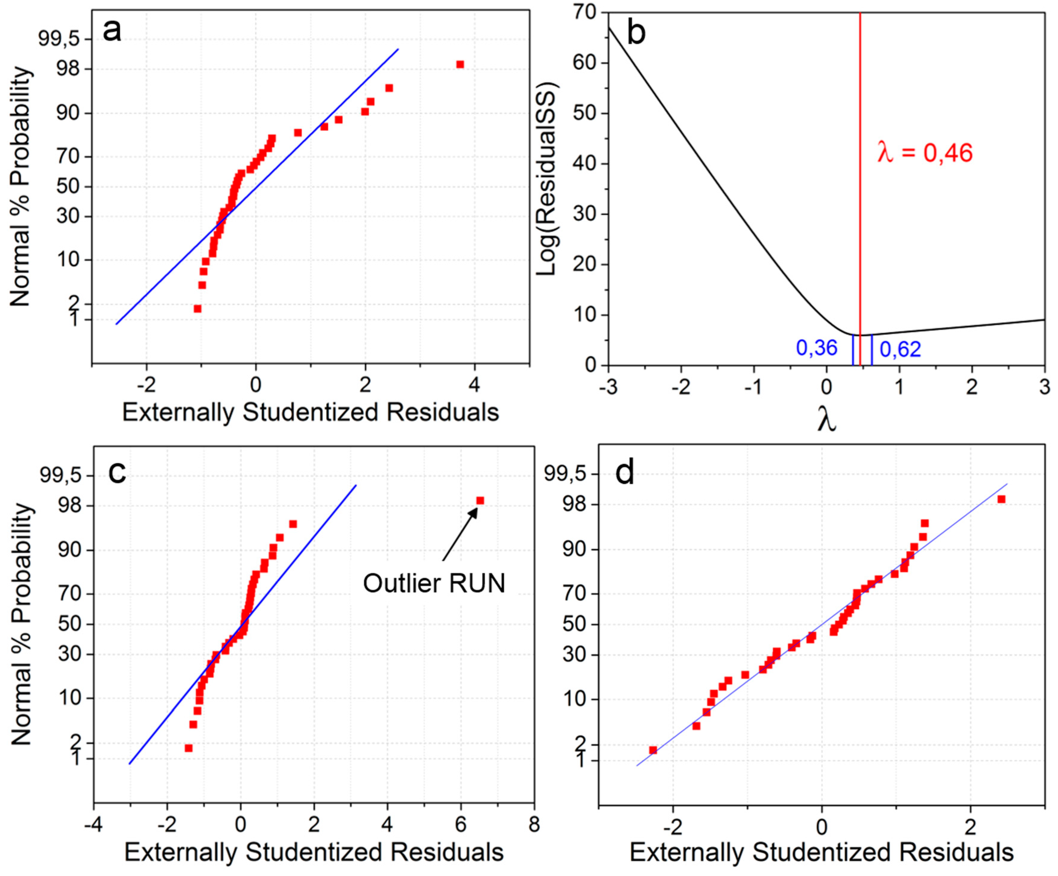
The normal probability plot of residuals is a powerful tool to seek outliers as well as to confirm the normal distribution of the experimental data. It plots the cumulative normal probabilities, or
z-score, against their externally studentized residuals. As shown in
Figure 5a,c,d, the blue line represents the predicted values and should serve as a guideline for the residuals’ distribution. The Box-Cox method represented in
Figure 5b is well-adapted to determining which transformation might bring the most normality to the dataset. It plots the residual sum of squares as a function of
λ, the transformation coefficient.
In
Figure 5a, the left tail (negative studentized residuals) is much longer than the right tail (positive studentized residuals); the data is skewed left, which is a sign of a non-normal distribution. This can be mitigated by applying a variance-stabilizing transformation to the data and modifying Equation (3) into Equation (4):
where
k and
λ are real numbers. Statistical methods such as DoE only provide an objective analysis of the likelihood that a given factor has an impact on the process. Hence, if the transformation normalizes the distribution, it should be used even if a physical interpretation of the transformation is not yet possible. The best transformation to apply can be inferred from the Box-Cox representation in
Figure 5b. The curve’s minimum, marked by the red vertical line, represents the value of
λmin for which
Yλ has the most normal distribution, and the 95% confidence interval is comprised between the two blue vertical lines. For
λmin = 1, no transformation is necessary. In the case of
λmin = 0, the transformation yielding the best normality would be log(
Y). Aside from these two, all other values suggest a power transformation. In
Figure 5b, the Box-Cox method indicates that the dataset would be more normal with a power transformation of
λ = 0.46. The additive term
k is generally used if some values are not strictly positive.
Figure 5c presents the same dataset after the transformation. The data is no longer skewed (both tails are of equal length), but normality is still not achieved since one residual sits very far from its predicted value. Therefore, this experimental run is a possible outlier and should be repeated for validation. If reformulating a new electrode did not provide normality to the data and if the standard deviation of the replicated measurements is within acceptable bounds, it would be worth investigating why and how the model diverges so much at this candidate point. In our case, binder content had a more than anticipated impact on high-current capacities, and its content should be minimized. This very strong impact could be further investigated in a new DoE by studying the squared effect of binder content on electrochemical performance.
In
Figure 5d, the transformed data with the outlier removed from the dataset shows residuals that essentially define a straight line: the response has a normal distribution and no outlier may be identified. The S-shape formed by points on the bottom left and top right does not necessarily indicate outliers, but rather the fact that some residuals were smaller than expected and thus that the distribution is not strictly normal, yet it is still normal enough for analysis.
The final step towards building a meaningful empirical model is an analysis of the descriptive statistics for all polynomial equations which fit the experimental values. Descriptive statistics are necessary to evaluate the proper fit of the resulting empirical models. The statistical tools will involve the analysis of variance (ANOVA) and the most common such statistic is R2. Unfortunately, R2 always increases with an increasing polynomial order, and thus could provide false confidence in models.
One solution is to adjust R2 by considering the number of factors in relation to the number of runs. This Adjusted R2 decreases when a higher-order model has less impact on the response than noise; it is the percentage informing on how much the variations in the response are attributed to individual model terms, e.g., x1 or x1 × x2. A second relevant coefficient is the Predicted R2, a statistic which describes how well the model can predict new experiments; it is calculated by removing an experimental data point, drawing an alternate empirical model and comparing the predicted value versus the missing observation. Negative Predicted R2 indicates the model is trying to fit the random noise, which is a sign of an overfit model, i.e., a model which no longer accurately describes the various factors’ influence. In such cases, a lower-order model should be sought, and the study of interactions should be left to a follow-up DoE in a smaller design space.
Ideally, the difference between the Adjusted R
2 and the Predicted R
2 should be less than 0.2. When this figure is higher than 0.2, the model is significantly overfitting the data and the experimenter should consider adding runs to identify remaining outliers and strengthening the model. To assess the statistical significance of the model, i.e., that the measured values are not random, the Model F-value and individual term’s
p value [
5,
6,
7] must be used in conjunction with R
2. The former helps reject the null hypothesis, i.e., “the data is not influenced by the factors”, i.e., the empirical equation is compared to a hypothetical model with all coefficients equal to 0. A value as high above one as possible would guarantee that most of the observations can be explained with the current model. For their part,
p values describe the probability for individual model terms, e.g.,
x1 or
x1 ×
x2, to not be significant. Usually, a 5% or lower chance is sought after, and a term with a
p value of 0.1 or higher is generally considered insignificant. If half or more of all
p values are greater than 0.1, model reduction should be considered to ensure a robust model is drawn. Finally, the signal-to-noise ratio, calculated by comparing the range of predicted values to the average prediction error, should be greater than 4 to guarantee satisfactory model discrimination.
Choosing the best model is an iterative process.
Table 1 outlines its different steps: the chosen model order and transformation are in the first column, and the various descriptive statistics pertaining to these choices are in the subsequent ones. The optimal variance-stabilization transformation was first sought after for linear and quadratic models; cubic or non-linear models were not investigated as the plan had not been designed to study such higher-order interactions. The quadratic model had the highest descriptive statistics to best describe capacities when the electrode was under high currents: new experiments can be predicted with 89% accuracy based on the Predicted R
2. Moreover, the binder type was proven to have a significant importance for this response, so two empirical equations were drawn, with the one for Binder 2 (
B2) being Equation (5):
For λ > 0, Yλ is an increasing function for real numbers, i.e., if Yλ is positive, then Y is also positive and vice versa. Hence, an increase in Y0.46 signifies an increase in the value of the capacity. Conversely, if λ < 0, any increase in Yλ would result in a decrease in Y.
It must be noted that the p values were calculated on 20 individual terms: as the binder type was found to have a significant effect on the capacity, the significance of each of the 10 terms found in Equation (5) was additionally calculated in regards of the binder type, e.g., AM and AM × binderType. In this case study, two terms were marginal and had p values between 0.05 and 0.1 for the quadratic model with λ = 0.46. Finally, the p values determined that two-thirds of the factors are significant, meaning that the capacity at high current is very well described by interactions.
Moreover, our example is a particular case where the percentages of all the component of the mixture are within the same range. This allowed to directly compare the significance of the impacts. If this is not the case, the equation can also be computed using coded variables where the range of each factor is normalized between −1 and 1.
2.7. Analyzing the Model
Once the empirical model is appropriately precise, the impact of the different factors on the response may be analyzed. The modeled response for a four-component mixture design can only be represented in a regular tetrahedron. It is therefore impossible to represent the variations of a response on a two-dimensional medium. Instead, cross-sections of the volume can be displayed, representing one component fixed at a chosen level, and the three others varying.
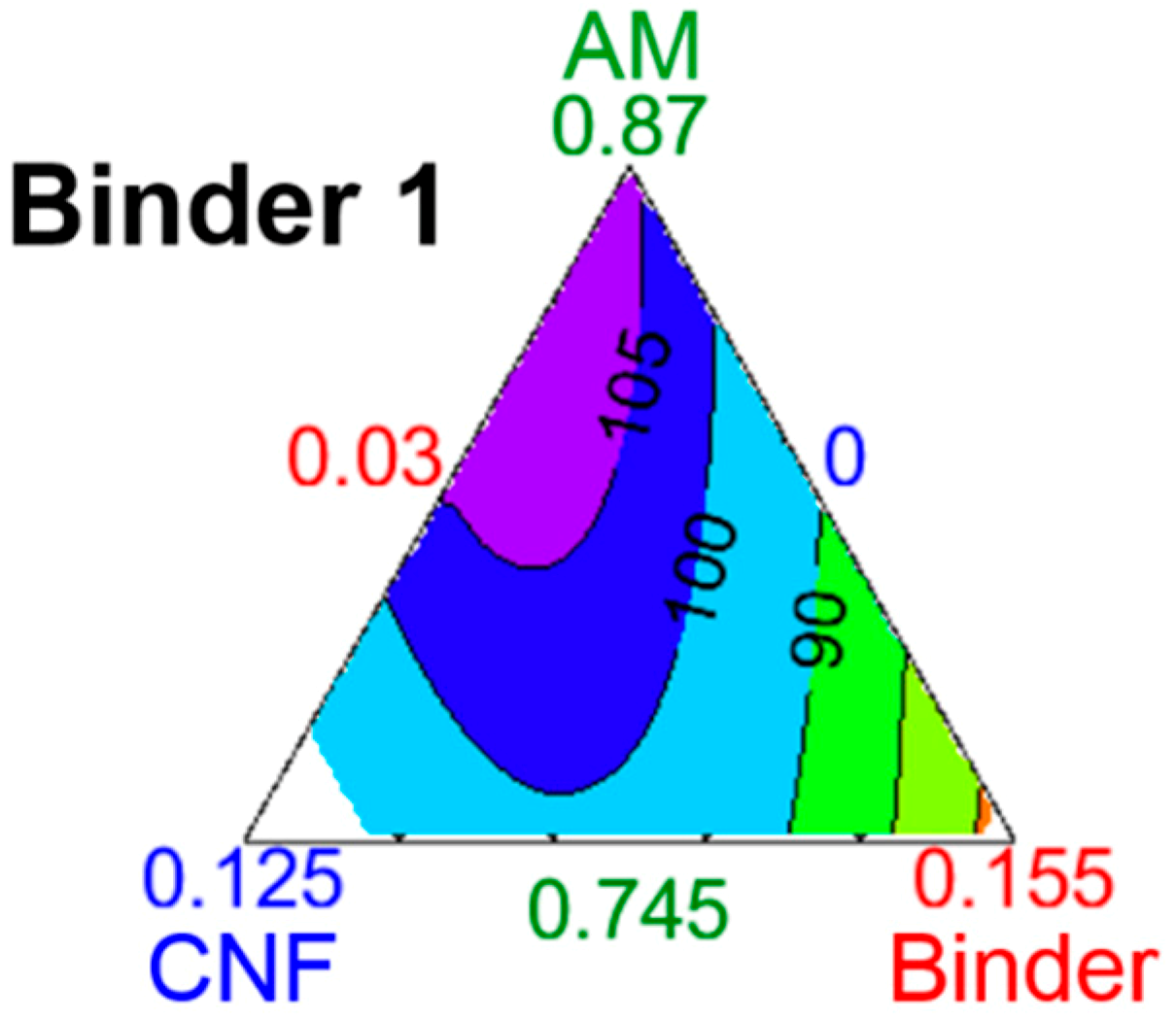
The most visual way to present these results is with an equilateral triangle.
Figure 6 illustrates the impact of the formulation on capacity with the carbon black (CB) content set at 20%
w. The colored areas in the triangles are separated by iso-capacity lines, in milliampere hour per gram of electrode, noted as mAh⋅g
−1.
A component’s content in the mixture, in %
w indicated by the numbers in the corresponding color, varies along the height from each summit. For example, in
Figure 6 the bottom left angle is related to the CNF. The closer the orthogonal projection of a point onto the height is to that summit, the higher the CNF-content in the mixture. Inversely, the closer it is to the opposite edge, the lower the CNF-content, down to 0%
w. In
Figure 6 for Binder 1, the iso-capacities are almost parallel to the CNF baseline, and thus the capacity is almost solely dependent on the CNF content with 20%
w of CB. On the other hand, in
Figure 6 for Binder 2, the iso-capacities are perpendicular to the AM baseline, and therefore the capacity is independent of the AM content with 20%
w of CB. Depending on the binder, the behavior of the capacity with regard to formulation is thus very different.
2.8. Drawing Conclusions
Working with a Design of Experiments is an iterative process. When setting up the design, choices were made in order to reduce the number of runs. These included the definition of the potential design and nuisance factors, and the focus on a limited number of interactions. To fully understand the process, it is often necessary to revisit the DoE with, for example, fewer materials or reduced ranges, which in turn would help improve precision. Another possibility is to investigate more complex factor behaviors, such as mapping terms with squared or exponential effects, or study higher-order interactions. If the ultimate objective is to predict the optimal point that yields the best response, it may be relevant to plan a new design, and select the candidate points with the best I-optimality.
Additionally, it is only possible to draw conclusions inside the design space for systems with similar characteristics. For example, electrodes with an AM loading between 4 and 4.5 mg⋅cm
−2, porosity between 40 and 50%
v, 20%
w of CB, and Binder 1 must maximize their CNF content and, more importantly, minimize Binder 1 content to achieve the highest possible capacity. However, this conclusion does not hold true when the CB content is reduced to 10%
w, as seen in
Figure 7. Here, the iso-capacities have a more complex shape and represent the interactions between the electrode’s components. The white area in the plot is outside of the study’s boundary: the CNF was set to vary from 0 to 10%
w, but the study’s constraints and the practicality of using an equilateral triangle show a domain from 0 to 12.5%
w of CNF. The area of maximum capacity, over 105 mAh⋅g
−1, is at the top of the diagram; this means that in this new system, the binder and CNF contents must be minimized to maximize capacity. This is likely because 10%
w of CB is enough to limit electrode polarization at high currents, and the AM content is so important that lowering it in favor of more conductive carbons is detrimental to overall capacity. In other words, the improved electronic and ionic (through decreased tortuosity [
29]) conductivity provided by the carbon nanofibers is insufficient to compensate for the loss of lithium intercalation sites. Finally, reaching such high capacities with a binder content of 3%
w suggests that Binder 1 is very efficient at providing mechanical cohesion to an electrode with a high powder volume.

 ,
, 


