Article

Estimation Accuracy and Computational Cost Analysis of Artificial Neural Networks for State of Charge Estimation in Lithium Batteries

1
Department of Mechanical and Aerospace Engineering, Politecnico di Torino, Torino 10129, Italy
2
Podium Advanced Technologies, Pont Saint Martin 11026, Italy
*
Authors to whom correspondence should be addressed.
Batteries 2019, 5(2), 47; https://doi.org/10.3390/batteries5020047
Submission received: 1 April 2019 / Revised: 2 May 2019 / Accepted: 7 May 2019 / Published: 1 June 2019

Abstract

:
This paper presents a tradeoff analysis in terms of accuracy and computational cost between different architectures of artificial neural networks for the State of Charge (SOC) estimation of lithium batteries in hybrid and electric vehicles. The considered layouts are partly selected from the literature on SOC estimation, and partly are novel proposals that have been demonstrated to be effective in executing estimation tasks in other engineering fields. One of the architectures, the Nonlinear Autoregressive Neural Network with Exogenous Input (NARX), is presented with an unconventional layout that exploits a preliminary routine, which allows setting of the feedback initial value to avoid estimation divergence. The presented solutions are compared in terms of estimation accuracy, duration of the training process, robustness to the noise in the current measurement, and to the inaccuracy on the initial estimation. Moreover, the algorithms are implemented on an electronic control unit in serial communication with a computer, which emulates a real vehicle, so as to compare their computational costs. The proposed unconventional NARX architecture outperforms the other solutions. The battery pack that is used to design and test the networks is a 20 kW pack for a mild hybrid electric vehicle, whilst the adopted training, validation and test datasets are obtained from the driving cycles of a real car and from standard profiles.

1. Introduction

Increasing concerns about global warming as well as oil and resource depletion have led to more stringent regulations linked to fuel economy, emissions, and energy conservation. In the automotive industry, this has created an incentive to focus efforts on alternative powertrain technologies [1]. In this context, the development of battery systems has gained a sizable momentum [2,3] due to their fundamental role in fully electric, hybrid and plug-in hybrid electric vehicles (BEVs, HEVs, PHEVs). Amongst the variety of battery chemical combinations, lithium batteries have few competitors today because of their remarkable properties in terms of efficiency, compact size and weight, fast charging, and low self-discharge rate [4,5,6]. Nevertheless, lithium battery performance and health are severely affected by the number and type of the charge/discharge cycles, and also by environmental factors such as temperature and age. Moreover, lithium batteries require constant and accurate monitoring to check their condition, specifically, the level of the remaining available energy, indicated by the SOC. An accurate and reliable knowledge of the SOC mitigates psychological factors such as the range anxiety associated with electric vehicles. Additionally, it contributes to prevent accelerated battery ageing due to deep discharge, overheating, and overcharging. However, the SOC cannot be directly measured, and its value can only be estimated from the measurement of other battery parameters, such as current, voltage, internal resistance, and temperature. Common laboratory techniques for SOC estimation are based on the measurement of open circuit voltage, internal impedance of the battery, or on current integration over time [7,8]. These approaches are also known as direct methods. Although accurate, these methods are energy consuming, not compatible with fast discharge rates, and therefore, are not suitable for real-time applications [9]. To overcome these issues, model-based, rule-based and artificial intelligence-based techniques have been proposed in recent research findings. The first family includes the Kalman Filter (KF) [10], Extended Kalman Filter (EKF) [11,12,13,14], Unscented Kalman Filter (UKF) [15,16], Adaptive Particle Filter (APF) [17], and Smooth Variable Structure Filter (SVSF) [18,19]. These solutions exploit the aforementioned direct methods for tuning of the reference model and are heavily dependent on its accuracy [9]. Rule-based techniques, such as Fuzzy Logic (FL) [20,21,22], do not need any model but are strictly dependent on the experience of the algorithm designer. In this context, Artificial Intelligence-based solutions like Artificial Neural Networks (ANNs) have gained increasing attention as they are reliable and robust, independent from the cell chemistry, suitable for the representation of nonlinear dynamics and compatible with real-time applications [9]. Nevertheless, the effectiveness and the accuracy of an ANN is strongly dependent on the adopted architecture and on the selection of proper training datasets. An additional issue is that the resulting network may be too heavy in terms of memory occupation and processing time, demanding high performance computing units to be correctly deployed. To the authors’ knowledge, the analysis of the computational cost of the ANNs deployed on real control units and validation in real driving cycles profiles are considered to be missing points in the literature. Indeed, several architectures have been proposed, although they have weak validations that are attained by means of simple laboratory charge/discharge profiles and without addressing the computational cost analysis. Feedforward ANNs have been proposed in both standard configurations [23,24] and in combination with UKF [25] and EKF [11]. These works presented a validation based on periodic laboratory discharge profiles. Additionally, their computational cost during training and deployment is not investigated. Similarly, an Elman ANN is studied in [26] without a validation in real driving cycle profiles, where there is no discussion on the weight of the algorithm. The NARX architecture is proposed in [27] with a validation conducted on periodic charging/discharging cycles that are characterized by simple profiles (trapezoidal and triangular wave in charging and discharging respectively). These profiles do not explore a significant range of the battery dynamics and present levels of current in the range of ±15A, which are far from real conditions that are around an order of magnitude higher. Moreover, this work does not investigate the computational cost, as well as the divergence issue due to the initial SOC inaccuracy, which is typical in such a layout.
Therefore, the aim of this paper is to fill the gap in the literature by presenting a trade-off analysis between the performance of five different ANNs for SOC estimation. The ANNs are trained and tested using real driving cycle profiles to determine their computational cost during training and deployment. Two of the ANNs are already available in the literature: Feedforward Non Linear Input-Output [11,23,24,25] and the Recurrent Elman ANN [26]. In this study, they are considered as a reference. The third ANN is a NARX, which has been previously proposed for SOC estimation in [27] using a standard configuration. Here, it is presented in an unconventional layout as it includes a starting routine that avoids the inherent output error due to an inaccurate estimate of the initial feedback. The other two ANNs are the Multi-Layer Cascade Feedforward and the Multi-Layer Recurrent networks, which are selected because they have proven to be effective in executing estimation tasks in other fields.
The trade-off between the five ANNs is carried out in terms of estimation accuracy, as well as duration and performance of the training process. Additionally, the networks are deployed on an electronic control unit that is similar to those adopted in Battery Management Systems (BMS) to analyze the computational cost in terms of execution time, as well as processor and memory occupation. Finally, the estimator performance is tested when the initial SOC is not accurate and the current measurement is affected by noise.
The test and validation tasks are performed on a lithium battery pack for mild-hybrid automotive applications. The training and test datasets are acquired on a real vehicle, and the performance and computational cost are evaluated on a portion of the “United States Advanced Battery Consortium” (USABC) PHEV dynamic charge depleting duty cycle profile [28].
In summary, the novel contributions of this work are: (1) trade-off analysis between different ANN architectures in terms of estimation accuracy and computational cost; (2) validation of the method on real driving cycle profiles; (3) adoption of an unconventional NARX network to avoid estimation divergence issues due to the SOC initial value inaccuracy.

2. Artificial Neural Network Design

Typically, the design of ANNs consists of three phases: training, test and validation. The training phase is conducted exploiting datasets reproducing the widest possible range of the system dynamics to allow an accurate learning. In this study, the training datasets include the current, voltage and temperature measurements as network inputs and the SOC as the output target. Since the SOC is a non-measurable quantity, its value is obtained from a look-up table battery model tuned by means of the Ampère-hour counting method performed in a laboratory environment. This model (block 1 in Figure 1) is then used as an emulator of the real battery to generate the expected SOC reference. The proposed ANNs architectures (block 2) are designed and simulated in the Matlab/Simulink environment and then deployed on a real electronic control unit with a Hardware in the Loop (HIL) configuration (block 3) based on an Atmel AVR 8-bit processor in serial communication with a computer. The calculation performance of this processor is comparable to that of common BMSs.
The design procedure can be summarized as follows: (a) the training input dataset (current, voltage and temperature) is provided to block 1 to obtain the training output target ( S O C _ 1 ); (b) block 2 is fed with the obtained input/output dataset to perform the ANN training procedure; (c) the test and validation steps are conducted by providing new datasets to the three blocks and comparing the outputs from the reference model of block 1 with the trained ANN model of block 2 and block 3. The feedforward ANNs do not require feedback of the output estimation, while the recurrent ANNs exploit the feedback of the SOC estimation as the fourth input (dashed line in Figure 1).
The adopted battery pack is composed of 168 cells KOKAM SLPB 11543140H5 in the configuration 12p14s (p: parallel, s: series). The pack has a nominal voltage of 48 V, a nominal capacity of 60 Ah, and is designed for a mild-hybrid electric vehicle with a peak electric power of around 20 kW, obtained considering a discharge rate of around 7C in nominal conditions. The main characteristics of the cell are reported in Table 1.

2.1. ANN Proposed Architectures

The study is performed by comparing the performance of five different ANN architectures: Feedforward Linear Input-Output (Figure 2a), Multi-Layer Cascade Feedforward (Figure 2b), Recurrent Elman ANN (Figure 2c), Multi-Layer Recurrent ANN (Figure 2d) and NARX (Figure 3). For each of the architectures, the activation functions, number of layers, delays d , and number of neurons are found by means of a trial-and-error procedure, as the best compromise between estimation accuracy, time of training, and need to avoid training overfitting. The activation functions are the sigmoid or hyperbolic tangent functions for the hidden layers H A F , and the linear function for the output layers O A F . The network training function for each architecture is the Levenberg-Marquardt [29].
The first two ANNs of Figure 2 are the feedforward configurations, where the information flows in one direction from the input to the output nodes, without forming any recurrent cycle.
The Non-Linear Input-Output network (Figure 2a) is the simplest configuration included in this study, and is designed with a single hidden layer consisting of 10 neurons, d x = 2 , a sigmoid H A F and a linear O A F . Essentially, the output y ( n ) of this network is the result of applying a non-linear function φ to the inputs x ( n ) , according to the following equation:
y ( n ) =   φ [ x ( n 1 ) , x ( n 2 ) ,   ,   x ( n   d x ) ]
where φ is the non-linear function modeled with the ANN.
The Multi-Layer Cascade Feedforward network (Figure 2b) exploits the formulation defined by Equation (1). Each layer takes both the input and output of all previous ones as inputs. Further theoretical details can be found in [30]. The proposed configuration includes three hidden layers (12, 10 and 8 neurons, respectively), with no delays on the inputs. The activation functions of the hidden and output layers are the hyperbolic tangent and linear functions, respectively.
In the recurrent Elman ANN (Figure 2c), the output of the hidden layer is fed back as an input of the same layer. The designed network features eight neurons in the hidden layer, d x = 1 and d y = 1 , and the sigmoid and linear activation functions for the input and output layers, respectively. Basically, this network produces an output y ( n ) according to the following equation:
y ( n ) =   φ [   x ( n   d x ) , ;   ϕ ( x ( n   d y ) ) ]
where φ is the non-linear function modeled by the ANN, and ϕ is the function executed by the hidden layer to the input x ( n ) . A detailed theoretical background can be found in [31] and in [32].
The Multi-Layer Recurrent network (Figure 2d), is designed with three hidden layers (5, 4 and 2 neurons, respectively), d x = 2 and d y = 2 , a sigmoid H A F and a linear O A F . The output y ( n ) is computed by applying a non-linear function φ , which is modeled by the ANN network, to the inputs x ( n ) , as in the following equation:
y ( n ) =   φ [ x ( n 1 ) ,   x ( n   d x ) ;   ϕ 1 ( x ( n 1 ) ,   x ( n   d y ) ) ; ;   ϕ i ( x ( n 1 ) ,   x ( n   d y ) ) ]
where the output of each i -hidden layer is fed back as an additional input of the same layer. A thorough background on recurrent ANNs can be found in [33].
The last architecture (Figure 3) is the NARX. This network is represented by a discrete nonlinear model and is commonly used for time series prediction tasks. It is defined as:
y ( n ) = φ [ y ( n 1 ) , y ( n 2 ) , , y ( n d y ) ; x ( n 1 ) , x ( n 2 ) , , x ( n d x ) ]
where y ( n ) and x ( n ) denote the outputs and inputs of the NARX model at the discrete timestep n , respectively. d x and d y are the input and output memory used in the model, respectively, and φ is the function, generally non-linear, represented by the ANN. During the NARX regression procedure, the next value of the dependent output signal y ( n ) is regressed on the previous d y values of the output signal and previous d x values of the independent (exogenous) input signal. In the proposed solution, the NARX is adopted in open loop (Figure 3a) during the training process, and in closed loop (Figure 3b) during the estimation phase, i.e., when the network is deployed in the real application. The open loop configuration is also known as Series-Parallel (SP) mode. In this configuration, the output regressor is:
y ( n ) = φ [ y ¯ ( n 1 ) , y ¯ ( n 2 ) , , y ¯ ( n d y ) ; x ( n 1 ) , x ( n 2 ) , , x ( n d x ) ] .
In this case, a supervised training procedure is conducted using the true output as target. This has some advantages: The input of the artificial neural network is more accurate and the resulting network has a purely feedforward architecture, so a static backpropagation algorithm (Levenberg-Marquardt) can be used for the training process.
The closed loop configuration, also called Parallel (P) mode, where the output estimation is:
y ( n ) = φ [ y ( n 1 ) , y ( n 2 ) , , y ( n d y ) ; x ( n 1 ) , x ( n 2 ) , , x ( n d x ) ] .
When using the network in the Parallel mode, at the beginning of the computation, the estimation has an undetermined value and cannot be fed back to the ANN input because it would make the estimation diverge over time. To overcome this issue, during the first second of the computation, the feedback signal is replaced by a constant value ( S O C I N I T in Figure 3b) that is the last SOC value recorded on a non-volatile memory at the previous shut down of the system. After the first second of the computation, i.e., when the output estimation is stable, the input related to the SOC switches to the feedback signal.
Referring to Figure 3b and denoting n = n 0 , the time instant when the feedback signal switches from S O C I N I T to the estimated output, the characteristic equation of the model are written as:
y ( n ) = φ [ S O C I N I T ; x ( n 1 , x ( n 2 ) , , x ( n d x ) ) ] , n < n 0
and
y ( n ) = φ [ y ( n 1 ) , y ( n 2 ) , , y ( n d y ) ; x ( n 1 ) , x ( n 2 ) , , x ( n d x ) ] ,   n n 0 .

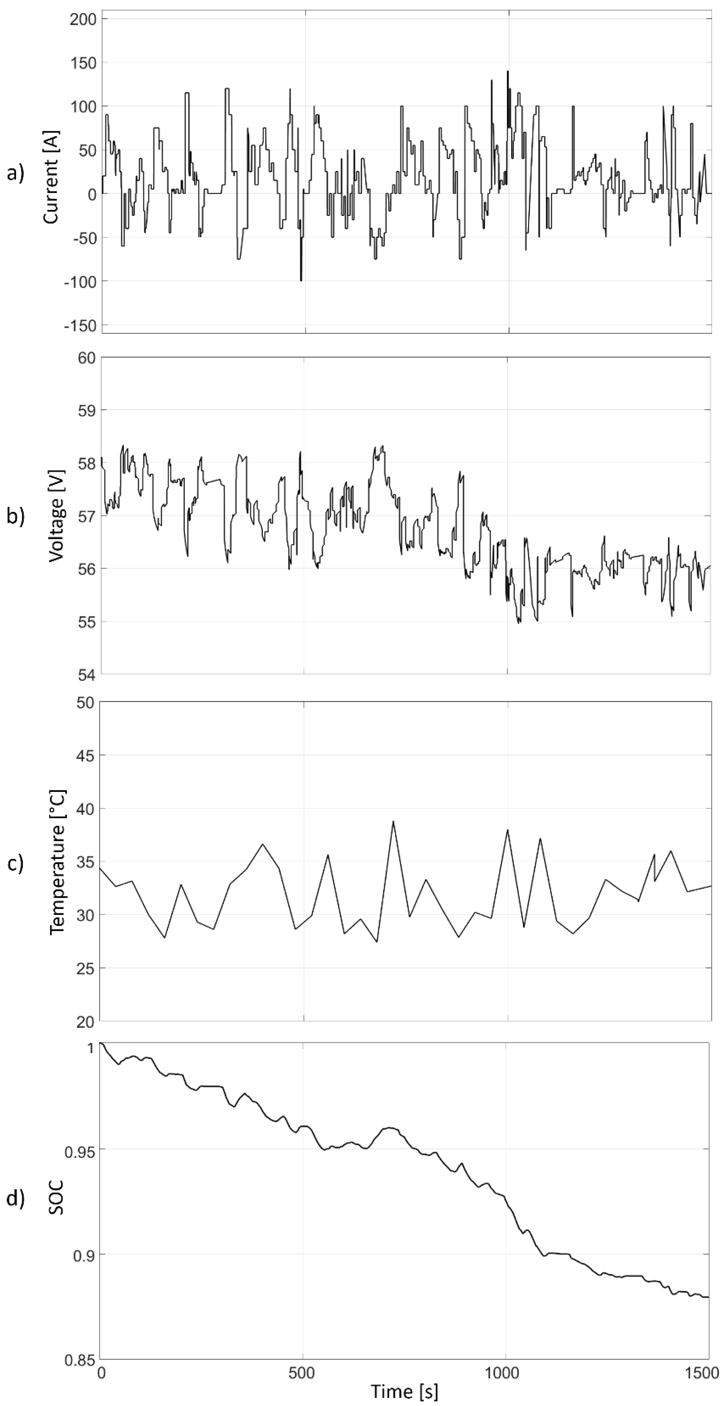
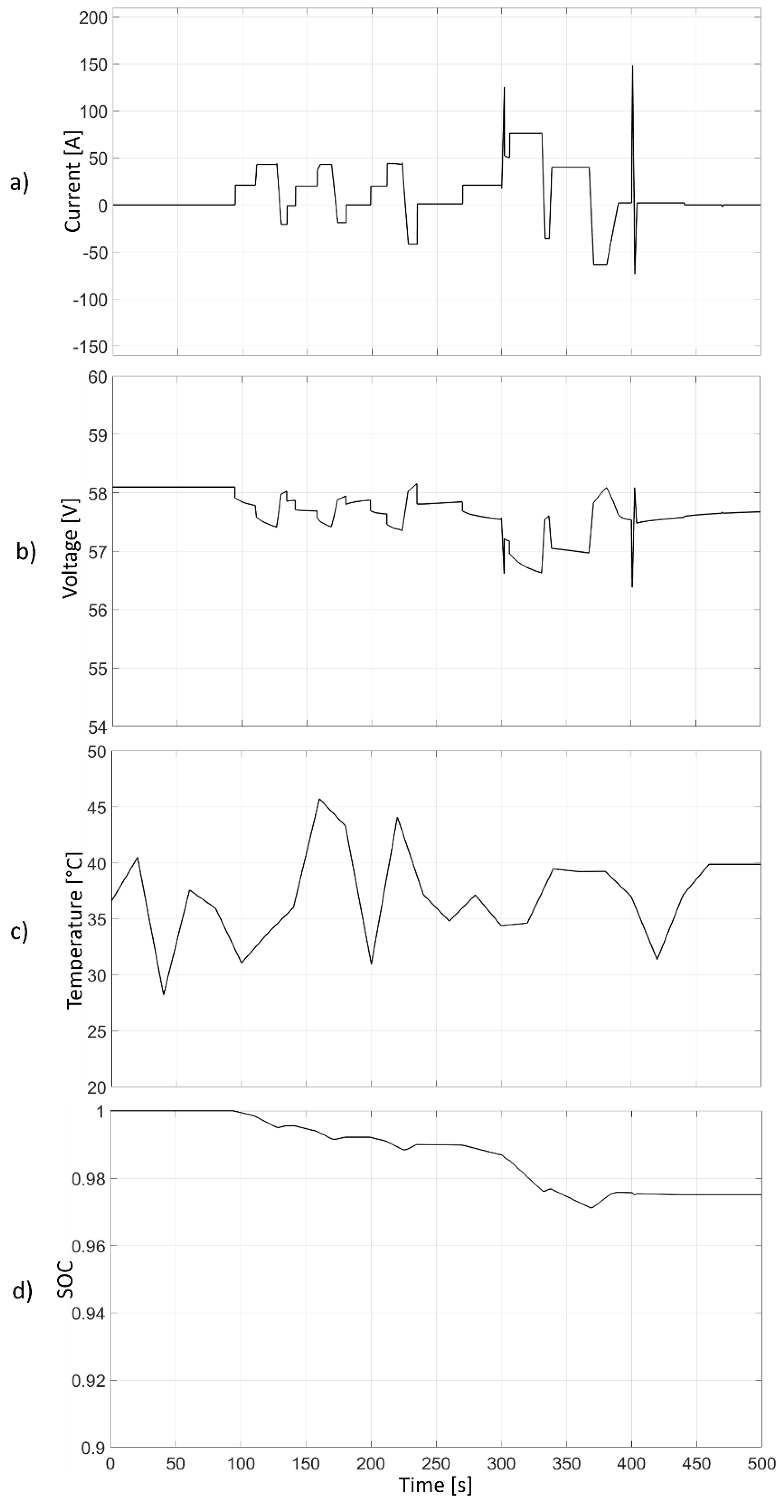
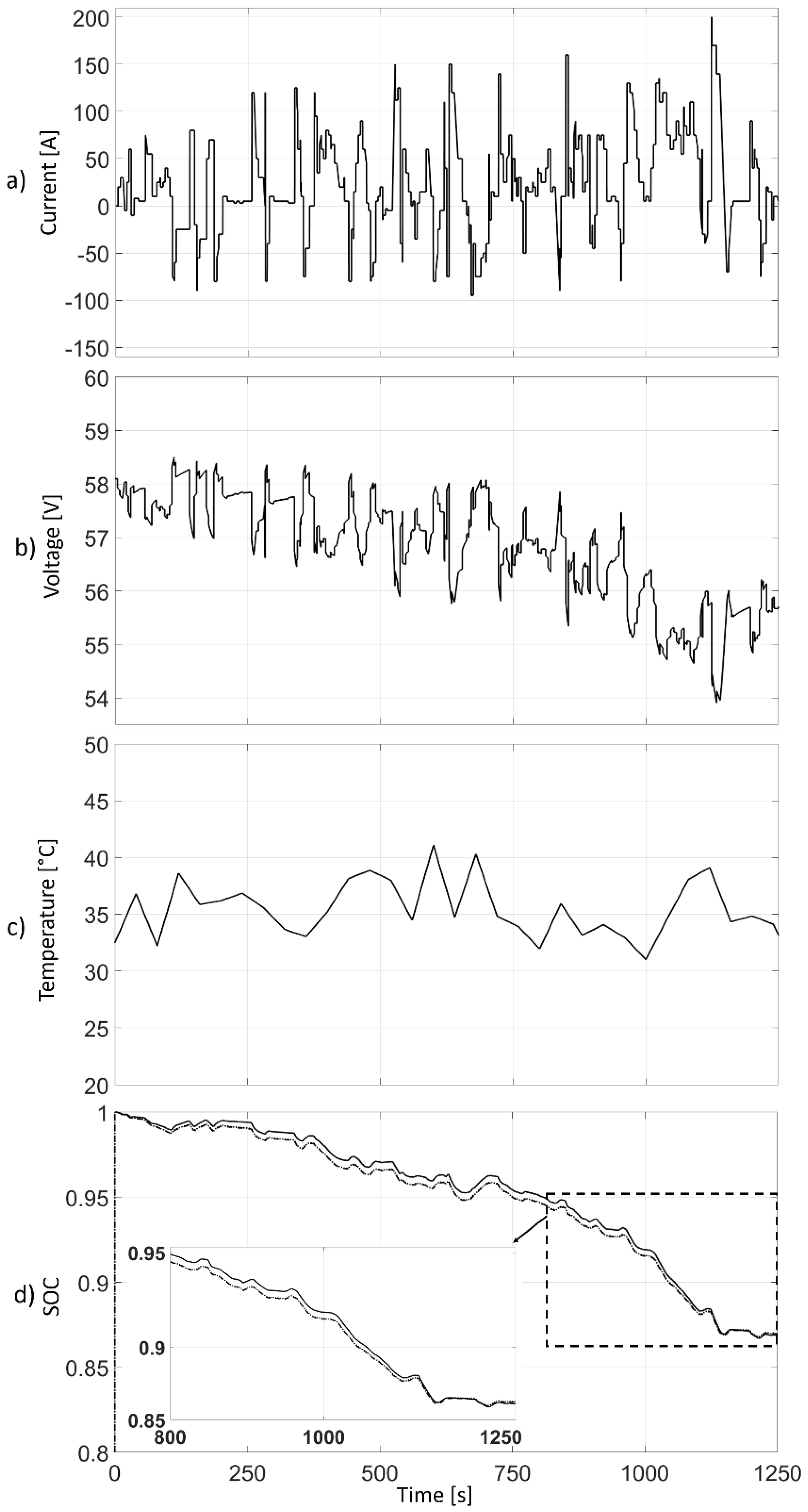
2.2. Training and Test Datasets

The adopted training dataset is obtained from a current charge/discharge profile of a real EV that is reported in [34]. The dataset is shown in Figure 4, where the values of the voltage (Figure 4b), temperature (Figure 4c) and SOC (Figure 4d) are obtained from the reference model (the block 1 in Figure 1) when the input of the model is the current (Figure 4a). The data are sampled with a frequency of 10 Hz. Since this profile produces a reduction of SOC equal to 12.5%, it is replicated eight times in the training dataset to obtain a full discharge of the battery.
The test dataset is a portion of the “United States Advanced Battery Consortium” (USABC) PHEV dynamic charge depleting duty cycle profile [28], reported in Figure 5. It is adopted to evaluate training and estimation accuracy, and the computational cost analysis of the five proposed ANN architectures.

3. Results and Discussion

The proposed ANNs are tested using the dataset reported in Figure 5. The aim is to evaluate the method performance in terms of duration and precision of the training process, estimation accuracy, and computational cost. The latter is analyzed by measuring the memory and processor occupation, when the designed algorithms are deployed on an electronic control unit. Finally, the estimation accuracy and robustness of the ANN is evaluated with an additional profile obtained from a real electric vehicle.

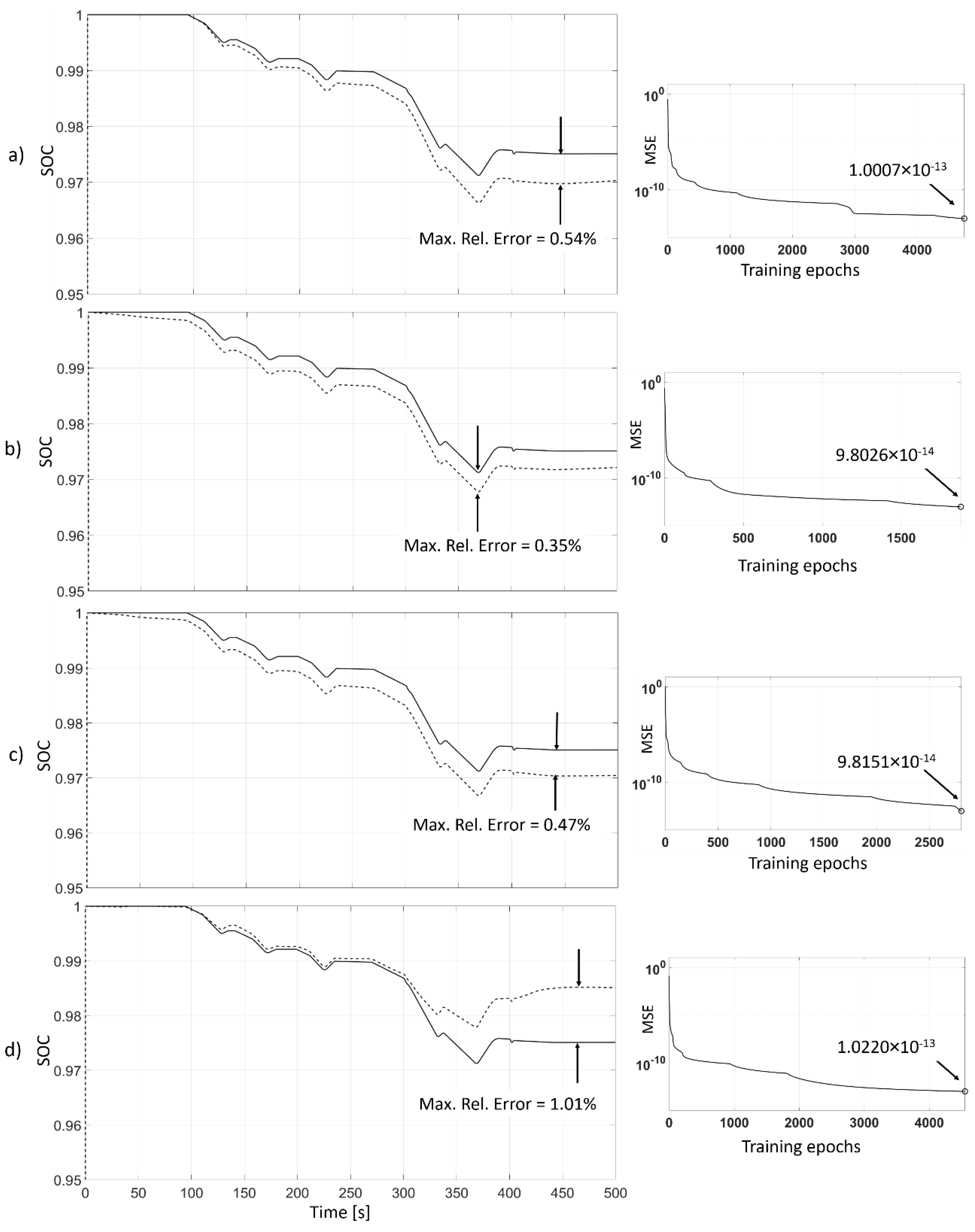
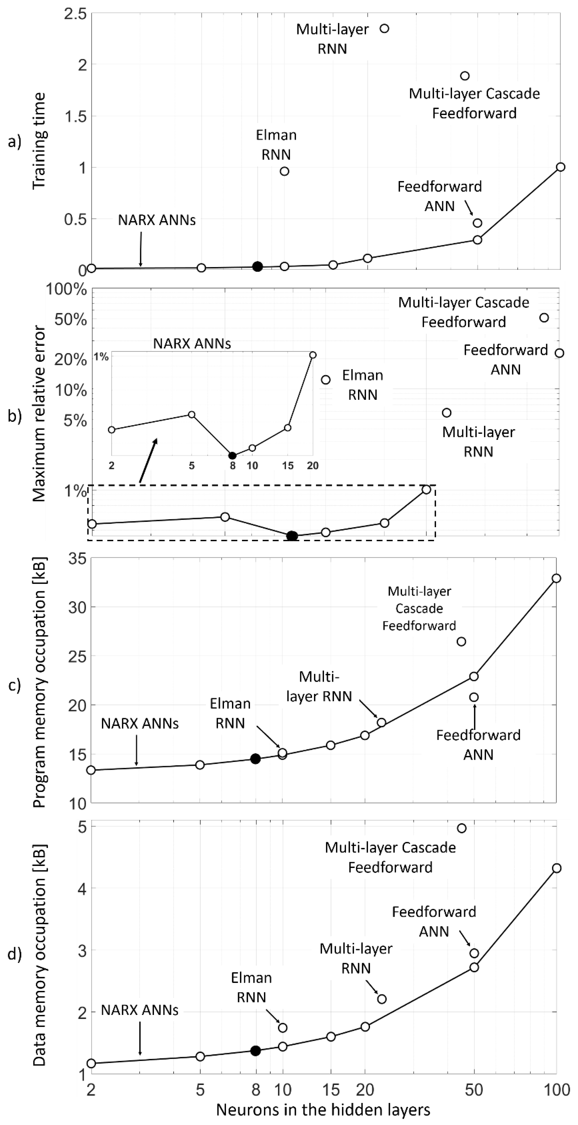
3.1. Performance and Computational Cost Analysis

The first test is conducted to analyze the estimation accuracy, and training precision and duration. The latter is computed in a number of training epochs for each ANN. The estimation accuracy is analysed by means of the Maximum Relative Error (MRE), computed as:
MRE   [ % ] = max 1 < i < n ( | S O C e x p ( i ) S O C e s t ( i ) S O C e x p , m a x = 1 | ) · 100 ,
where n is the number of the measurements, S O C e x p and S O C e s t are the expected and estimated SOC, respectively.
On the other hand, the training accuracy is evaluated by means of the Mean Square Error (MSE) obtained at the end of the learning process. The training is stopped when the MSE is equal to or lower than 1   ×   10 13 or, alternatively, when it remains constant for a sufficiently large number of training epochs.
Figure 6 reports the results obtained by the Feedforward Linear Input-Output, Multi-Layer Cascade Feedforward, Recurrent Elman ANN, and Multi-Layer recurrent ANN. The training process of each of these networks is stopped because the training MSE does not reduce after one hundred epochs. Each ANN is tested using a configuration that results to be the best in terms of number of neurons, layers, delays and activation/training functions. This is achieved by a trial-and-error procedure. Different configurations, i.e., with a larger number of neurons and layers produce worse results in terms of training duration and accuracy, especially when overfitting occurs. The plots on the left-hand of Figure 6 show that none of these networks provides a sufficiently accurate SOC estimation. The recurrent ANNs (Elman SRN and Multi-layer RNN) are characterized by slightly better results with respect to the feedforward ANNs (Linear Input-Output and Multi-Layer Cascade). Nevertheless, the zoomed portions in (Figure 6c) and (Figure 6d) show evidence that the estimated SOC (dashed line) is inaccurate (MRE around 5%) when compared to the expected one (solid line).
The performance of the NARX ANNs with one layer and 5, 8, 15 and 20 neurons in the hidden layer are presented in Figure 7. The training of each network is stopped because the MSE reaches enough small value. The network with the best performance is the NARX with eight neurons (Figure 7b). It has the minimum training MSE ( 9.8   ×   10 14 ), reached with the lowest number of training epochs, and minimum estimation error MRE (0,35%).
The results obtained with all the proposed architectures are summarized and compared in Figure 8, where the NARX with eight neurons is marked with a black circle. The plots in the first row show the performance of the networks in terms of duration of the training process (Figure 8a) normalized with respect to a NARX with one layer and 100 neurons, and of SOC estimation in terms of MRE (Figure 8b). In this second plot, the results of the NARX with 50 and 100 neurons are not reported because of the high simulation time required, and performance that deteriorates at increasing the number of neurons. In general, NARX architectures show a lower training time and better estimation performance when compared with other solutions. The results reported in (Figure 8c) and (Figure 8d) allow comparing the tested networks in terms of computational cost when they are deployed on an electronic control unit with an Atmel AVR-8 bit microcontroller, which is similar to those adopted in common BMSs.
During this test, the measurements of current, voltage and temperature are emulated by means of a computer and sent in serial communication to the control unit. The output estimation is sent back via serial communication to the computer for monitoring and data logging tasks. The occupation of the program memory (Figure 8c) and data memory (Figure 8d) are measured in kB and reported on a logarithmic scale as function of the number of neurons contained in the hidden layers of each ANN. As expected, the required computational power increases with the complexity of the network, but this demand is generally acceptable for deployment on a real BMS.
Finally, the accuracy of the NARX with eight neurons is tested using a profile obtained from a real electric vehicle [33]. The results are reported in Figure 9, where the dynamics of the current profile (Figure 9a) are similar to those of the training dataset (Figure 4a) but reveals a more aggressive driving style with peaks that reach values of 200 A. The SOC estimation (Figure 9d) is accurate, and the MRE is lower than 0.35%, as expected from the results illustrated in Figure 7. The solid line in (Figure 9d) represents the expected SOC, while the dashed and dash-dotted lines are the estimated SOC in simulation and in the control unit, respectively. The good correspondence between the three lines is a validation of the correctness of the estimation and of the deployment setup. It is worthy to notice that the estimation is never higher than the expected value, which is a conservative situation, since it allows avoiding the over-estimation of the residual energy on the battery, which may represent a critical situation in EVs.

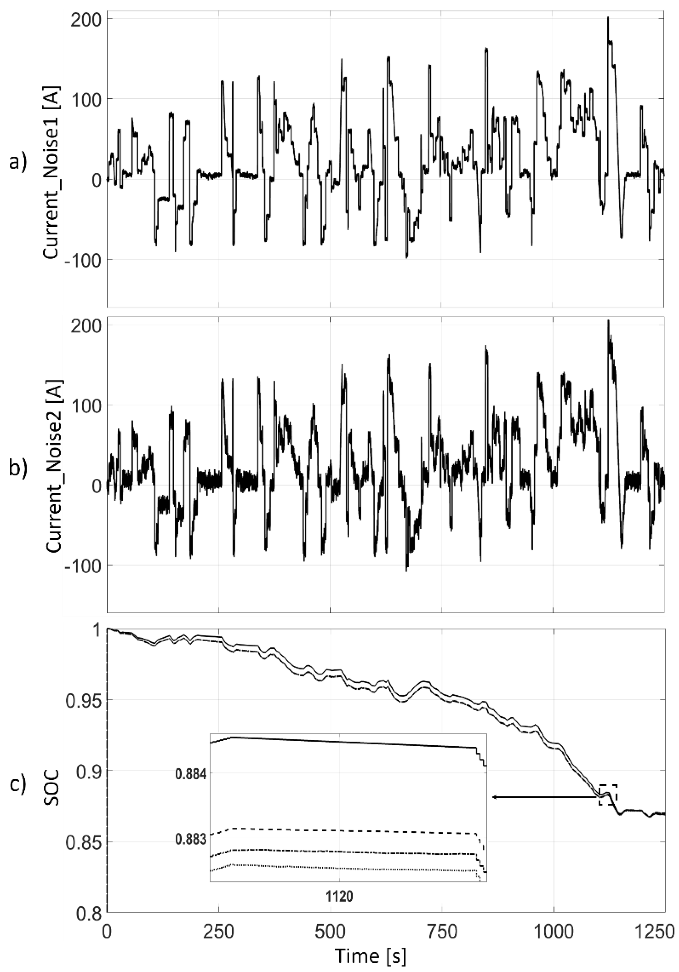
3.2. Robustness Analysis

The final test conducted on the NARX with eight neurons aims to evaluate its robustness when the initial value of the SOC ( S O C I N I T in Figure 3b) is not accurate and when the current measurement is affected by noise, which is a typical condition in real applications.
The first analysis is carried out by introducing a relative error in the maximum tolerance range of ± 5 % on the S O C I N I T and evaluating the capabilities of the network to recover this error or at least to keep it limited in between the lower and upper tolerance thresholds. The test is conducted adopting a portion of the validation dataset reported in the zoomed area of Figure 9d, and testing the robustness in a range of ± 5 % , centred on S O C = 95 % . The results are reported in Figure 10, where the estimation behaviour and trend of the error are reported in (Figure 10a) and (Figure 10b), respectively, and the error tolerance region is coloured in grey. The plots show that the estimation tends to converge to the expected value or to remain constant in the case of errors lower than 4%, whilst the estimation can diverge and exceed the tolerance range in the case of larger errors.
The second analysis is conducted by disturbing the measurement of the current provided as input to the network. Two different types of noise are summed up in the current profile of Figure 9: A 1 kHz pseudo-random Gaussian noise having zero mean value and standard deviation equal to 1.5 A (type 1, Figure 11a) and a 100 Hz pseudo-random Gaussian noise having zero mean value and standard deviation equal to 5 A (type 2, Figure 11b). The results are reported in (Figure 11c), where the solid line is the expected value, the dashed line is the estimation without noise and the dash-dotted and dotted lines are the estimation affected by the type 1 and type 2 noise, respectively. The results show that the estimation performance is not affected by problems of noise on the current measurement, which is typically the most disturbed signal in the real applications. Obviously, the ANN does not have the capabilities to effectively compensate possible inaccuracies in the offset and gain calibration of the current sensors.

4. Conclusions

In this paper, a trade-off analysis between five different ANN architectures for the SOC estimation of lithium batteries of hybrid and electric vehicles has been presented. The study was conducted to evaluate the estimation accuracy, duration of the training process, robustness to the noise on the current measurement, and deployment computational cost. Two analyzed architectures, Feedforward and Elman ANNs, were already reported in the SOC estimation literature, unlike the multi-layer recurrent and Cascade-forward. The last proposed architecture was NARX with an unconventional architecture to guarantee the accuracy of the initial SOC value. The networks have been trained and tested with real driving cycles obtained from an electric vehicle. The NARX architecture resulted in the most performance in terms of estimation error, training time and computational cost (program and data memory lower than 15 kB and 1.5 kB, respectively), featuring a maximum estimation error of 0.35%. Additionally, an analysis conducted by perturbing the estimation initial value showed that the NARX architecture was robust for initial errors lower than 4%, while the estimation diverged in the other cases.

Author Contributions

A.B., S.F., A.T. and N.A. contributed to the conceptualization and definition of the estimation layout. F.M. realized the reference model of the battery. A.B and S.F designed the ANNs and validated the method experimentally. A.B., S.F., A.T. and N.A contributed to the writing and editing of the manuscript.

Funding

The presented research activity has been conducted in the framework of the project “High Efficiency Hybrid Powertrain”, partially funded by Regione Valle d’Aosta.

Conflicts of Interest

The authors declare no conflict of interest.

References

  1. Bishop, J.D.K.; Martin, N.P.D.; Boies, A.M. Cost-effectiveness of alternative powertrains for reduced energy use and CO2 emissions in passenger vehicles. Appl. Energy 2014, 124, 44–61. [Google Scholar] [CrossRef]
  2. Walther, G.; Wansart, J.; Kieckhafer, K.; Schneider, E.; Spengler, T.S. Impact assessment in the automotive industry: Mandatory market introduction of alternative powertrain technologies. Syst. Dyn. Rev. 2010, 26, 239–261. [Google Scholar] [CrossRef]
  3. Ahman, M. Assessing the future competitiveness of alternative powertrains. Int. J. Veh. 2003, 33, 309. [Google Scholar] [CrossRef]
  4. Chan, C.C.; Chau, K.T. Modern Electric Vehicle Technology; Oxford University Press: New York, NY, USA, 2002. [Google Scholar]
  5. Anderman, M. Status and Trends in the HEV/PHEC/EV Battery Industry; Rocky Mountain Institute: Snowmass, CO, USA, 2008. [Google Scholar]
  6. Chen, X.; Shen, W.; Vo, T.T.; Cao, Z.; Kapor, A. An overview of lithium-ion batteries for electric vehicles. In Proceedings of the IEEE IPEC Conference on Power and Energy, Ho Chi Minh City, Vietnam, 12–14 December 2012. [Google Scholar]
  7. Leksono, E.; Haq, I.N.; Iqbal, M.; Soelami, F.N.; Merthayasa, I. State of Charge (SoC) Estimation on LiFePO4 Battery Module Using Coulomb Counting Methods with Modified Peukert. In Proceedings of the IEEE 2013 Joint International Conference on Rural Information & Communication Technology and Electric-Vehicle Technology, Bandung, Indonesia, 26–28 November 2013. [Google Scholar]
  8. Chang, W.Y. The State of Charge Estimating Methods for Battery: A Review. Appl. Math. 2013, 2013. [Google Scholar] [CrossRef]
  9. Rivera-Barrera, J.P.; Muñoz-Galeano, N.; Sarmiento-Maldonado, H.O. SoC Estimation for Lithium-ion Batteries: Review and Future Challenges. Electronics 2017, 6, 102. [Google Scholar] [CrossRef]
  10. Wei, Z.; Zhao, J.; Ji, D.; Tseng, K.T. A multi-timescale estimator for battery state of charge and capacity dual estimation based on an online identified model. Appl. Energy 2017, 204, 1264–1274. [Google Scholar] [CrossRef]
  11. Charkhgard, M.; Farrokhi, M. State-of-Charge Estimation for Lithium-Ion Batteries Using Neural Networks and EKF. IEEE Trans. Ind. Electron. 2010, 57, 4178–4187. [Google Scholar] [CrossRef]
  12. Jiang, C.; Taylor, A.; Duan, C.; Bai, K. Extended Kalman Filter based battery state of charge (SOC) estimation for electric vehicles. In Proceedings of the IEEE Transportation Electrification Conference and EXPO (ITEC), Detroit, MI, USA, 16–19 June 2013. [Google Scholar]
  13. Pérez, G.; Garmendia, M.; Reynaud, J.F.; Crego, J.; Viscarret, U. Enhanced closed loop State of Charge estimator for lithium-ion batteries based on Extended Kalman Filter. Appl. Energy 2015, 155, 834–845. [Google Scholar] [CrossRef]
  14. Wang, S.; Fernandez, C.; Shang, L.; Li, Z.; Li, J. Online state of charge estimation for the aerial lithium-ion battery packs based on the improved extended Kalman filter method. J. Energy Storage 2017, 9, 69–83. [Google Scholar] [CrossRef]
  15. He, Z.; Chen, D.; Pan, C.; Chen, L.; Wang, S. State of charge estimation of power Li-ion batteries using a hybrid estimation algorithm based on UKF. Electrochim. Acta 2016, 211, 101–109. [Google Scholar]
  16. Yu, Q.; Xiong, R.; Lin, C. Online estimation of state-of-charge based on H infinity and unscented Kalman filters for lithium ion batteries. Energy Procedia 2017, 105, 2791–2796. [Google Scholar] [CrossRef]
  17. Ye, M.; Guo, H.; Xiong, R.; Yang, R. Model-based state-of-charge estimation approach of the Lithium-ion battery using an improved adaptive particle filter. Energy Procedia 2016, 103, 394–399. [Google Scholar] [CrossRef]
  18. Kim, T.; Wang, Y.; Sahinoglu, Z.; Wada, T.; Hara, S.; Qiao, W. State of Charge Estimation Based on a Realtime Battery Model and Iterative Smooth Variable Structure Filter. In Proceedings of the IEEE Innovative Smart Grid Technologies—Asia, Kuala Lumpur, Malaysia, 20–23 May 2014. [Google Scholar]
  19. Zou, Z.; Xu, J.; Mi, C.; Cao, B.; Chen, Z. Evaluation of Model Based State of Charge Estimation Methods for Lithium-Ion Batteries. Energies 2014, 7, 5065–5082. [Google Scholar] [CrossRef] [Green Version]
  20. Du, J.; Liu, Z.; Wang, Y.; Wen, C. A Fuzzy Logic-based Model for Li-ion Battery with SOC and Temperature Effect. In Proceedings of the 11th IEEE Conference on Control & Automation (ICCA), Taichung, Taiwan, 18–20 June 2014. [Google Scholar]
  21. Li, H.; Wang, W.; Su, S.; Lee, Y. A Merged Fuzzy Neural Network and Its Applications in Battery State-of-Charge Estimation. IEEE Trans. Energy Convers. 2007, 22, 697–708. [Google Scholar] [CrossRef]
  22. Lin, F.J.; Huang, M.S.; Yeh, P.Y.; Tsai, H.C.; Kuan, C.H. DSP Based Probabilistic Fuzzy Neural Network Control for Li-Ion Battery Charger. IEEE Trans. Power Electron. 2012, 27, 3782–3794. [Google Scholar] [CrossRef]
  23. Cai, C.H.; Du, D.; Liu, Z.Y.; Zhang, Z. Artificial neural network in estimation of battery state of-charge (SOC) with nonconventional input variables selected by correlation analysis. In Proceedings of the International Conference on Machine Learning and Cybernetics, Beijing, China, 4–5 November 2002. [Google Scholar]
  24. Soylu, E.; Soylu, T.; Bayir, R. Design and Implementation of SOC Prediction for a Li-Ion Battery Pack in an Electric Car with an Embedded System. Entropy 2017, 19, 146. [Google Scholar] [CrossRef]
  25. He, W.; Williard, N.; Chen, C.; Pecht, M. State of charge estimation for Li-ion batteries using neural network modeling and unscented Kalman filter-based error cancellation. Electr. Power Energy Syst. 2014, 62, 783–791. [Google Scholar] [CrossRef]
  26. Shi, Q.; Zhang, C.; Cui, N.; Zhang, X. Battery State-Of-Charge estimation in Electric Vehicle using Elman neural network method. In Proceedings of the IEEE 29th Chinese Control Conference (CCC), Beijing, China, 29–31 July 2010. [Google Scholar]
  27. Chaoui, H.; Ibe-Ekeocha, C.C. State of Charge and State of Health Estimation for Lithium Batteries Using Recurrent Neural Networks. IEEE Trans. Veh. Technol. 2017, 66, 8773–8783. [Google Scholar] [CrossRef]
  28. Fan, G.; Pan, K.; Canova, M. A Comparison of Model Order Reduction Techniques for Electrochemical Characterization of Lithium-ion Batteries. In Proceedings of the IEEE 54th Annual Conference on Decision and Control, Osaka, Japan, 15–18 December 2015. [Google Scholar]
  29. Moré, J.J. The Levenberg-Marquardt algorithm: Implementation and theory, Numerical Analysis. In Lecture Notes in Mathematics; Watson, G.A., Ed.; Springer: Berlin/Heidelberg, Germany, 1978; Volume 630. [Google Scholar]
  30. Warsito, B.; Santoso, R.; Yasin, H. Cascade Forward Neural Network for Time Series Prediction. J. Phys. Conf. Ser. 2018, 1025, 012097. [Google Scholar] [CrossRef]
  31. Seker, S.; Ayaz, E.; Turkcan, E. Elman’s recurrent neural network applications to condition monitoring in nuclear power plant and rotating machinery. Eng. Appl. Artif. Intell. 2013, 16, 647–656. [Google Scholar] [CrossRef]
  32. Elman, J.L. Finding Structure in Time. Cogn. Sci. 1990, 14, 179–211. [Google Scholar] [CrossRef]
  33. Caterini, A. A Novel Mathematical Framework for the Analysis of Neural Networks; UWSpace: Waterloo, ON, Canada, 2017. [Google Scholar]
  34. Rezvanizanian, S.M.; Huang, Y.; Chuan, J.; Lee, J. A Mobility Performance Assessment on Plug-in EV Battery. Int. J. Progn. Health Manag. 2012, 3, 12. [Google Scholar]
Figure 1. Layout of the training, test and validation setup: 1: Reference model obtained with Ampère-hour counting method in a laboratory environment. 2: ANN simulated in Matlab/Simulink environment. 3: Hardware in the Loop test with the ANN deployed on an electronic control unit in serial communication with a computer.
Batteries 05 00047 g001
Figure 2. Artificial Neural Network architectures designed and evaluated for SOC estimation. (a) Feedforward Non-Linear Input-Output; (b) Multi-Layer Cascade Feedforward; (c) Recurrent Elman ANN; (d) Multi-Layer recurrent ANN. x ( t ) : inputs (current, voltage and temperature), d x : delay on the inputs, d y : delay on the feedback signal. w : weights, b : bias, H A F : hidden activation function, O A F : output activation function, y ( t ) : output (SOC).
Batteries 05 00047 g002
Figure 3. NARX architecture. (a) Series-Parallel (SP) mode (open-loop configuration) for training. (b) Parallel (P) mode (closed-loop configuration) for estimation.
Batteries 05 00047 g003
Figure 4. Training profiles. (a) Current charge/discharge. (b) Voltage. (c) Temperature. (d) State of Charge.
Batteries 05 00047 g004
Figure 5. Test dataset obtained as a portion of the “United States Advanced Battery Consortium” (USABC) PHEV dynamic charge depleting duty cycle profile: (a) Current charge/discharge. (b) Voltage. (c) Temperature. (d) State of Charge.
Batteries 05 00047 g005
Figure 6. Performance of the first four proposed architectures. (a) Feedforward Linear Input-Output. (b) Multi-Layer Cascade Feedforward. (c) Recurrent Elman ANN. (d) Multi-Layer recurrent ANN. The SOC estimation and Mean Square Error trend during the training process of each network are reported in the left-hand and right-hand column, respectively.
Batteries 05 00047 g006
Figure 7. Performance of the closed loop NARX ANNs with 5 (a), 8 (b), 15 (c) and 20 (d) neurons in the hidden layer. The SOC estimation and Mean Square Error trend during the training process of each network are reported in the left-hand and right-hand column, respectively.
Batteries 05 00047 g007
Figure 8. Comparison of all the proposed architectures. (a) Training time normalized with respect to the 100 Neurons NARX. (b) Maximum Relative Error (MRE) of estimation. (c) Computational cost: program memory occupation. (d) Computational cost: data memory occupation. The black circle indicates the ANN with the best performance: NARX single layer, eight neurons.
Batteries 05 00047 g008
Figure 9. Validation on a real profile. (a) Current charge/discharge. (b) Voltage. (c) Temperature. (d) State of Charge: expected SOC (solid line), estimated SOC in simulation (dashed line) and estimated SOC on real electronic control unit (dash-dotted line).
Batteries 05 00047 g009
Figure 10. Robustness analysis to the initial SOC estimation inaccuracies. (a) Estimation output with error on the initial SOC ranging from 5 % to + 5 % . (b) Error between the expected and the estimated SOC. In both plots, the grey area indicates the error tolerance region of ± 5 % . The solid lines represent the expected SOC and the two tolerance thresholds. The dashed lines are the SOC estimations.
Batteries 05 00047 g010
Figure 11. Robustness to noise on the current measurement. (a) Current with type 1 noise. (b) Current with type 2 noise. (c) SOC: expected without noise (solid line), estimated without noise (dashed line), estimated when the current is disturbed by the type 1 noise (dash-dotted line) and estimated when the current is disturbed with the type 2 noise (dotted line).
Batteries 05 00047 g011
Table 1. Main characteristics of the cell KOKAM SLPB 11543140H5.
Typical Capacity (@ 0.5C, 4.2 V ÷ 2.7 V, 25 °C)5 Ah
Nominal Voltage3.7 V
Cut-off voltage2.7 V
Continuous current150 A
Peak current250 A
Cycle life (Charge/Discharge @ 1C)>800 cycles
Charge conditionMax. Current10 A
Voltage4.2V ± 0.03 V
Operating TemperatureCharge0 °C–40 °C
Discharge−20 °C–60 °C
Mass128.0 ± 4 g
DimensionThickness11.5 ± 0.2 mm
Width42.5 ± 0.5 mm
Length142.0 ± 0.5 mm

