Article

State of Charge Estimation of Power Battery Using Improved Back Propagation Neural Network

College of Mechanical Engineering, Xi’an University of Science and Technology, Xi’an 710054, China
*
Author to whom correspondence should be addressed.
Batteries 2018, 4(4), 69; https://doi.org/10.3390/batteries4040069
Submission received: 15 October 2018 / Revised: 14 November 2018 / Accepted: 22 November 2018 / Published: 11 December 2018

Abstract

:
Accurately estimating the state of charge (SOC) of power batteries in electric vehicles is of great significance to the measurement of the endurance mileage of electric vehicles, as well as the safety protection of the power battery. In view of lithium ion batteries’ nonlinear relation between SOC estimation and current, voltage, and temperature, the improved Back Propagation (BP) neural network method is proposed to accurately estimate the SOC of power batteries. To address the inherent limitations of BP neural network, particle swarm algorithm is adopted to modify the relevant weighting coefficients. In this paper, the lithium iron phosphate battery (3.2 V/20 Amper-Hour) was studied. Charge and discharge experiments were conducted under a constant temperature. The training data were used to construct the surrogate model using the improved BP neural network. It is noted that the accuracy of the developed algorithm is increased by 2% as compared to that of conventional BP. Finally, an actual vehicle condition experiment was designed to further verify the accuracy of these two algorithms. The experimental results show that the improved algorithm is more suitable for real vehicle operating conditions than the traditional algorithm, and the estimation accuracy can meet the industry standards to a greater extent.

1. Introduction

With the increasing global demand for energy conservation and environmental protection, electric vehicles have developed rapidly [1,2]. Power batteries serve as the driving core of electric vehicles. In order to ensure the safe use and service life of the battery as well as satisfy the user’s requirement of real-time monitoring, the power battery must be strictly and efficiently managed. Various battery management systems (BMSs) and their corresponding data management methods have been proposed [3,4]. Among them, accurate state of charge (SOC) estimation plays an important role in the prediction of electric vehicle range and the safety protection of power batteries [5,6]. Therefore, a reliable estimation algorithm for power batteries is urgently needed. However, battery SOC estimation is a complex nonlinear system model. Moreover, battery voltage, current, and temperature represent complex nonlinear relationship cycles, so the corresponding SOC estimation algorithm must take these factors into account [7,8]. At present, the main battery SOC estimation algorithms include the Coulomb counter method, the open circuit voltage method, the anti-time integral method, the Kalman filtering method [9], and the neural network method, etc. Huang et al. [10] gave a brief introduction to the advantages of the Coulomb counter method, which is easy to implement in practical conditions. However, the disadvantages of this method are also obvious, as its estimation is not accurate and it is easily impacted by the environment [11]. Zheng et al. [12,13] used low current open circuit voltage and incremental open circuit voltage two ways to observe the relationship between the open circuit voltage (OCV) and SOC. This approach was more accurate, but the precision still needs to be improved. Xu et al. [14,15] developed a battery management system in which the information sampling circuit, such as battery voltage and current, were considered. Moreover, the estimation of the battery SOC was completed based on the Amper-Hour integral method. Zheng et al. [16,17] proposed a differential voltage (DV) analysis based a universal battery model and two associated SOC estimation algorithms using extended Kalman filter (EKF) and particle filter (PF), respectively. Based on the natural cubic interpolation approach, the SOC of the battery was deduced from the DV curves of various cells at different aging levels, and the SOC-DV model was proposed. Guo et al. [18,19] employed a lithium iron phosphate battery as their research object and, based on the shortcomings of the traditional SOC estimation algorithm, an improved BP neural network algorithm was proposed, which has a certain effect in reducing the lithium iron phosphate battery SOC estimation error. Pan [20] proposed a novel open-circuit voltage model based on cubic-Hermite interpolation to update the state estimation. This method can effectively improve the accuracy of the extended Kalman filter. Li et al. [21] analyzed the values of relevant parameters in the formula of the ANN time integration using a lithium iron phosphate power cell as the research object. Mao et al. [22] investigated the defects of the estimation algorithm of traditional battery SOC; the extended Kalman filter method was used to estimate the SOC and put it into practical application. Sepideh et al. [23] employed an extended Kalman filter algorithm based on an electrochemical model that was developed to estimate the SOC of power cells. The results showed that this algorithm has high precision and strong adjustment ability, based on the experimental data of the discharge test. Yu et al. [24] used the wavelet neural network method to estimate the battery SOC, and the results showed that the wavelet neural network method has a good approximation effect and strong robustness. In summary, the battery SOC estimation algorithm can basically realize the simple estimation function of SOC at the present stage, but SOC estimation is limited by working conditions and defects in the algorithm. Therefore, there is room for further improvement in the estimation accuracy.
In this paper, a particle swarm optimization (PSO) algorithm is used to optimize and improve the neural network method in order to solve the problem of the SOC being prone to falling into local minimum when the BP neural network method is employed. Considering the voltage, current, temperature, and cycle attenuation of the battery, the accuracy of battery SOC estimation is further improved.

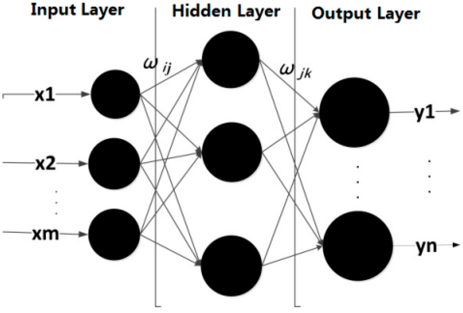
2. Back Propagation Neural Network Principle

Back propagation neural network is a multi-layer feedforward neural network model. The corresponding signal is forward-propagating, and the error can be reverse-transmitted and corrected [25]. The s-type function is used as the transfer function between neurons, and the range of network output values is (0, 1). Back propagation neural network can deal with complex nonlinear problems well, and can provide the appropriate network model according to different training data. The structure of back propagation neural network consists of a three-layer model, including an input layer, hidden layer, and output layer [26]. The back propagation neural network model is shown in Figure 1.
As you can see in Figure 1, the nerve cells between each layer interact with each other. If the mean square error between the output value from the output layer and the expected output value does not meet the set requirements, then reverse recurve and the correct weights and thresholds according to the principle of gradient descent can make the output value of the output layer meet the ideal requirements. The unit output of the corresponding neural network is shown in Equations (1) and (2).
P i = p ( i = 1 m ω i j x i + θ i ) j = 1 , 2 , l
Y k = q ( j = 1 l ω j k P i + θ k ) k = 1 , 2 , n
In the above equations, Pi represents the output of the hidden layer; Yk represents the output of the output layer; p and q respectively represent the transfer function of the hidden layer and the output layer; ωij is the connection weight between the input layer and the hidden layer; and ωjk is the connection weight between the hidden layer and the output layer. Moreover, m is the number of input layers; l is the number of hidden layers; n is the number of output layers; X = [x1, x2, ..., xm]T is the vector of input variables; and θ is threshold value. The mean square error calculated in the preceding feedback process is shown in Equation (3).
E = 1 2 k = 1 n ( t k y k ) 2 k = 1 , 2 , n
E represents the mean square error; tk represents the expected output; and Yk represents the actual output. In the process of error reverse transfer, weight correction follows Equation (4).
ω a + 1 = ω a η E ω a
ω a + 1 represents the correct weight; ω a represents the current state weight; and η represents the learning rate. Through continuous training and adjustment, the neural network can obtain the best training model, so that the mean square error can meet the set requirements. In the BP neural network method, the Levenberg Marquardt (LM) gradient descent algorithm is adopted to optimize the mean square error weight. This algorithm can effectively improve the convergence speed of BP neural network and reduce the prediction error value. Because the Hessian matrix is avoided, the calculated amount is greatly reduced, so the LM algorithm converges quickly. The problem is that the estimated error value falls into the local minimum value; it is not the optimal value. Therefore, it is necessary to improve the BP neural network, further revise the weight of the estimation process, and prevent the estimation value from falling into the extreme local minimum, so as to improve the accuracy of SOC estimation to a certain extent.

3. Improved Back Propagation Neural Network

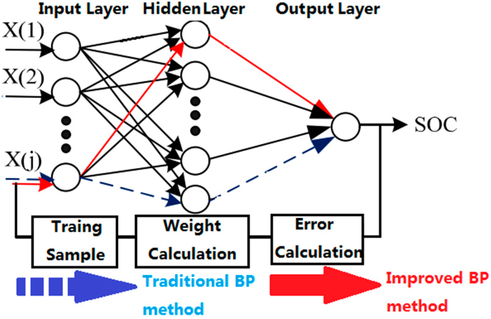
3.1. Improved Back Propagation Neural Network Principle

In order to solve the problem of estimating SOC by the LM steepest descent algorithm built in BP neural network, the particle swarm algorithm was adopted to re-optimize the weights in the training process. Particle swarm optimization is a method which can find the optimal intelligent solution. The PSO algorithm imitates the regularity of bird cluster activity. The optimal solution is obtained using the information of real-time sharing in the population to determine the optimal path. The position of the corresponding particle i is given as Xi = (Xi1, Xi2, Xij, ..., XiN), while the velocity is Vi = (Vi1, Vi2, Vij, ..., ViN), i ∈ [1, M], j ∈ [1, N]. The best position in the continuous space experienced by particle i is given as Pi = (Pi1, Pi2, …, PiN), and the optimal position of the particle in the global space is Ph = (Ph1, Ph2, Phj, ..., PhN). The corresponding velocity updating formula in particle swarm algorithm is expressed by Equation (5).
V i j ( t + 1 ) = ω V i j ( t ) + c 1 r 1 ( P i j ( t ) X i j ( t ) ) + c 2 r 2 ( P h j ( t ) X i j ( t ) )
Including the following variables: ω —Inertia weight; V i j ( t ) —Current particle velocity; t—Current iteration times; c1c2—Learning factor; r 1 , r 2 —[0.1] Uniformly distributed random numbers.
The corresponding position update formula is expressed by Equation (6).
X i j ( t + 1 ) = X i j ( t ) + V i j ( t + 1 )
The basic modeling of the improved BP neural network is the same as that of the traditional BP neural network. The difference is that the rules for adjusting and updating the weights and thresholds between the input layer and the hidden layer as well as between the hidden layer and the output layer are changed, as shown in Figure 2.
As can be seen in Figure 2, the improved BP neural network algorithm can quickly find the global optimal solution. The estimation error of SOC can be improved in theory. Corresponding weight and threshold correction follow Equations (7)–(10).
ω i j ( α + 1 ) = ω i j ( α ) + a η j X j
ω j k ( α + 1 ) = ω j k ( α ) + a σ k Y k
θ i ( α + 1 ) = θ i ( α ) + b η i
θ k ( α + 1 ) = θ k ( α ) + b σ k

3.2. Improved Back Propagation Neural Network Modeling

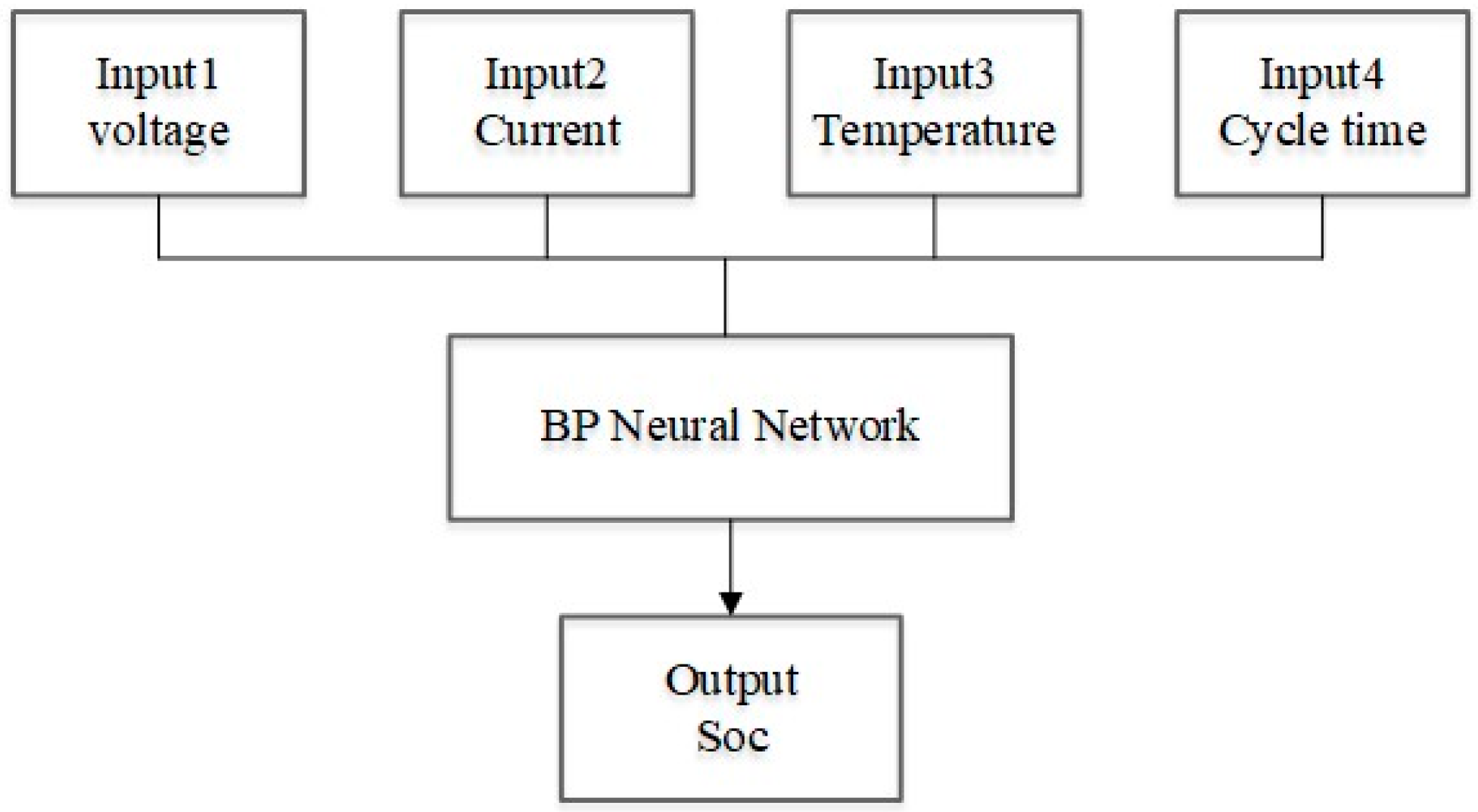
3.2.1. Input Layer Modeling

According to the research on the characteristics of the target battery, a battery’s SOC estimation is mainly affected by voltage, current, and environment temperature. At the same time, in order to correct the rate of a battery’s circulating capacity attenuation in a timely manner, the number of charge and discharge cycles of the battery was added to revise the SOC estimation. After comprehensive evaluation and analysis, the input layer was determined to include four neurons.

3.2.2. Hidden Layer Model

The number of nodes in the hidden layer and the number of layers are positively correlated with the complexity of the neural network. In general, the more nodes, the smaller the mean square error, and the more accurate of training. At the same time, the training time of the network will become longer and serious overfitting will occur. The number of nodes in the hidden layer is generally based on Equations (11) and (12), which are used to determine the approximate range.
l = log 2 m
l = n + m + a
Here, m is the number of input layer nodes; n is the output nodes number; and a is the adjustment coefficient, which is between 0 and 10. According to the empirical formula, the value of l is determined, and then different values at both ends of the l value are tried. According to the network training duration and the minimum mean square error, the number of hidden layers of the optimal combination is considered. Through the present experiment, the number of hidden layer nodes was set at 10, at which point the mean square error is relatively reasonable.

3.2.3. Output Layer Model

The final output variable is only the estimated value of the SOC, so the value of n is 1. We can set up the following network model, as shown in Figure 3.

4. Improved Back Propagation Neural Network Algorithm

Based on the original network model, the particle swarm algorithm is implanted. The specific steps of the algorithm are as follows:
(1)
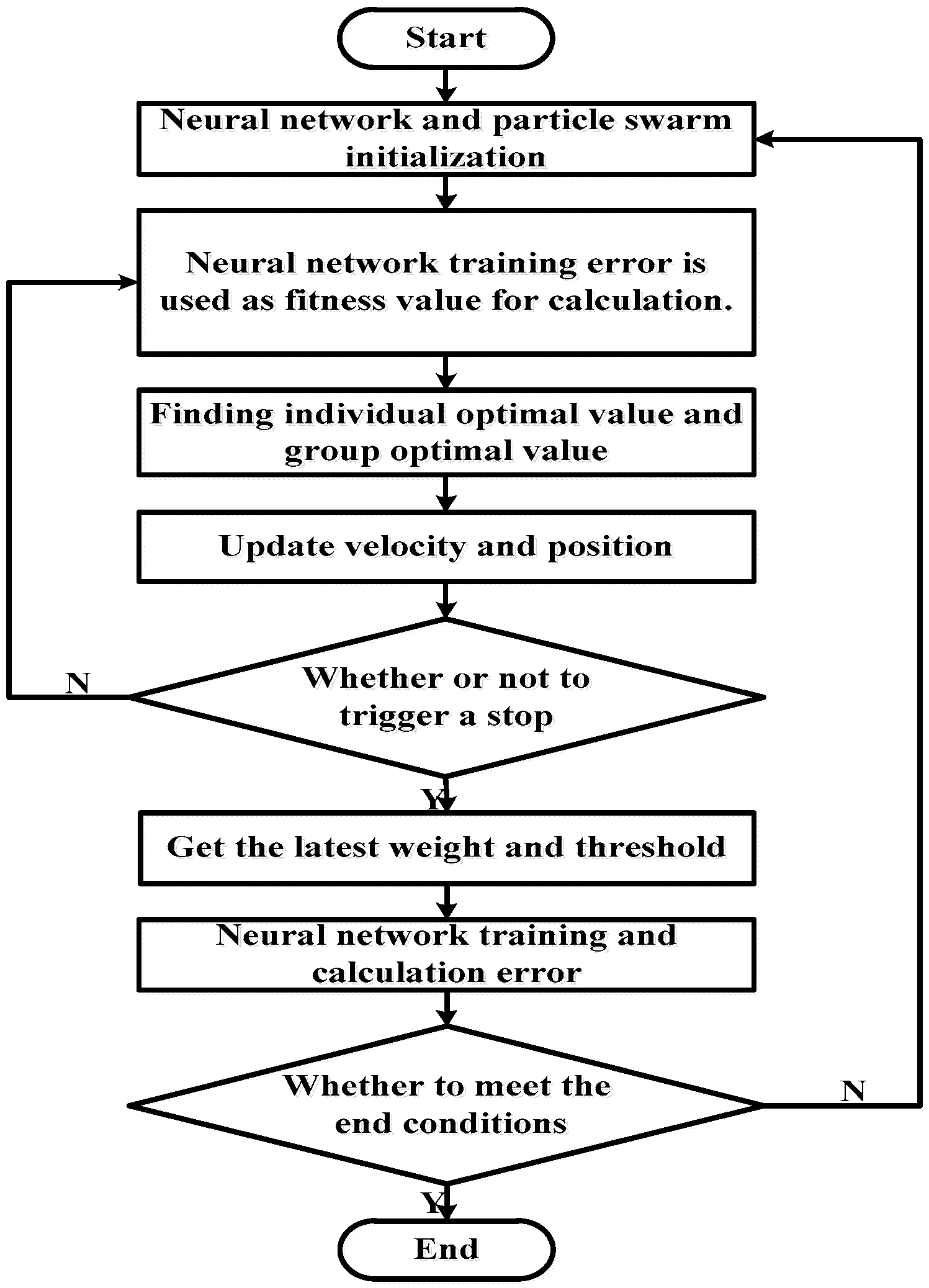
Initialize: first, the whole model is initialized to determine the particle size, setting particle velocity, location, global extremum, individual extreme value, and maximum number of iterations.
(2)
Neural network training: the initial state neural network training is conducted.
(3)
Determination of particle fitness: the feedback mean square error is fully utilized in neural network training, and then brought into the calculation as the fitness function value of the particle swarm.
(4)
Optimal value finding: the fitness value of each particle is compared with the optimal value of the individual in the current state, leaving the optimal result; in the same way, group optimal values are identified.
(5)
Update speed and location: the velocity and position of the particle swarm is updated according to Equations (5) and (6).
(6)
The particle algorithm ends: the end condition is the maximum number of iterations that has been set or the point at which N steps is reached, and the mean square error of all samples can meet the requirements. If the end condition is not met, the particle fitness determination step is repeated, and the sequence is carried forward step by step. When the requirements are met, the iteration is stopped and returned to the optimal individual. The optimal value of the individual particle is the improved neural network weight, and the global optimal value is used as the adjustment threshold.
(7)
Improved neural network model error analysis: this step determines whether the final mean square error and the SOC estimation error meet the requirements—the training will be finished if they are satisfied; if not, resetting and training is continued until the error requirements are met. The flow chart of the corresponding algorithm is shown in Figure 4.

5. Working Condition Test and Simulation Analysis

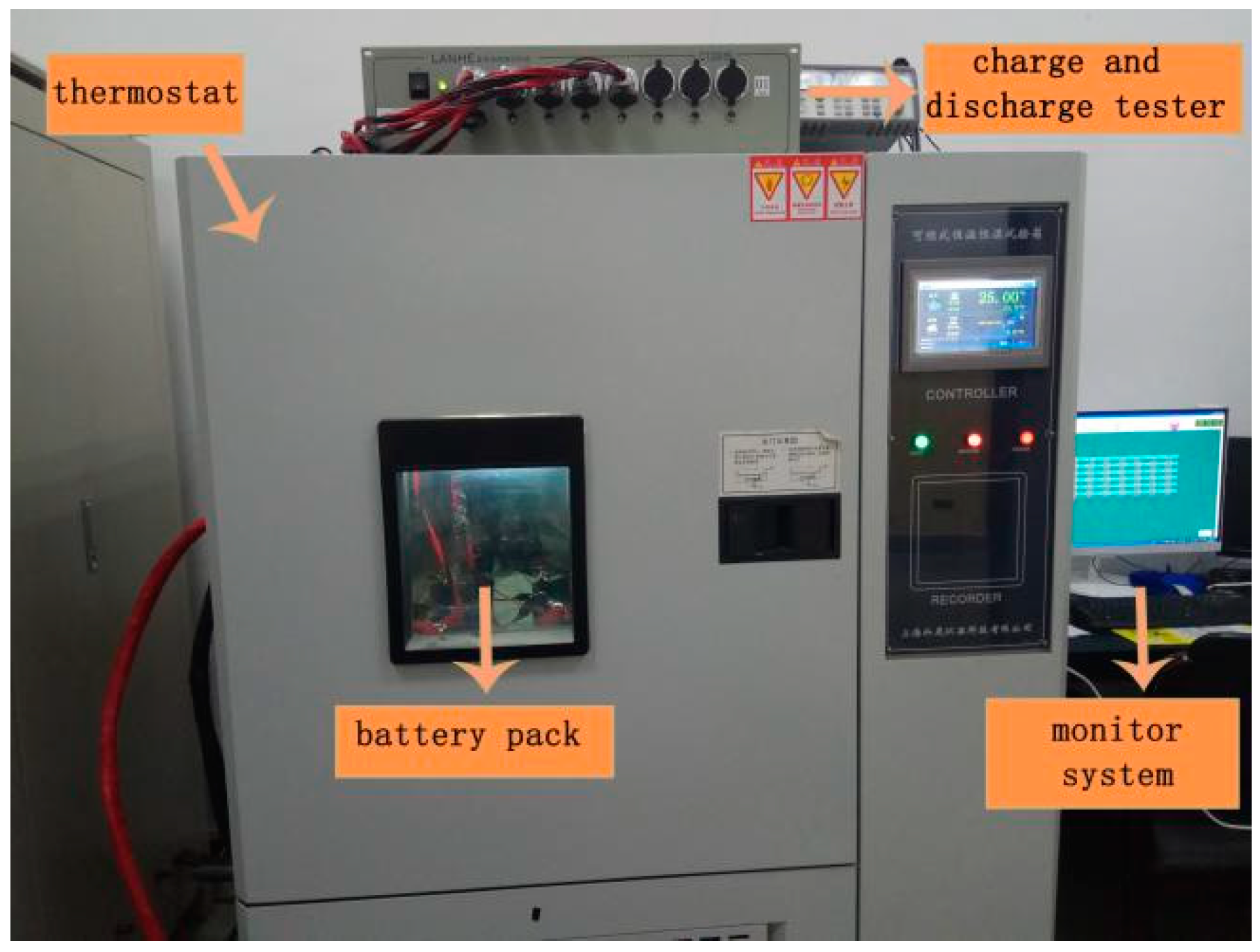
5.1. Construction of Experimental Platform and Training Sample Collection

In this paper, a prismatic lithium iron phosphate battery was selected as the research object. The nominal voltage was 3.2 V and the rated capacity was 20 Ah. The charging limit voltage was 3.65 V, the lower limit voltage was 2.5 V, and the maximum discharge current was 2 C. In this paper, all training samples were collected under a 1-C discharge rate. The experimental apparatus included a blue electric charge and discharge tester, a thermostat, and a computer. It is shown in Figure 5.
First, the thermostat temperature was set to 25 °C; the charge and discharge tester was used to charge the battery to full power in the charging mode of the constant current constant voltage (CCCV). After 30 min, discharge at the rate of 1 C current brought to the single battery voltage to 2.5 V, which indicates that the battery was discharged. During the test period, the tester recorded the voltage, current, and number of cycles every two seconds, and the thermostatic test box recorded the ambient temperature data [27,28]. Finally, the total number of training samples was determined to be 1500 groups.

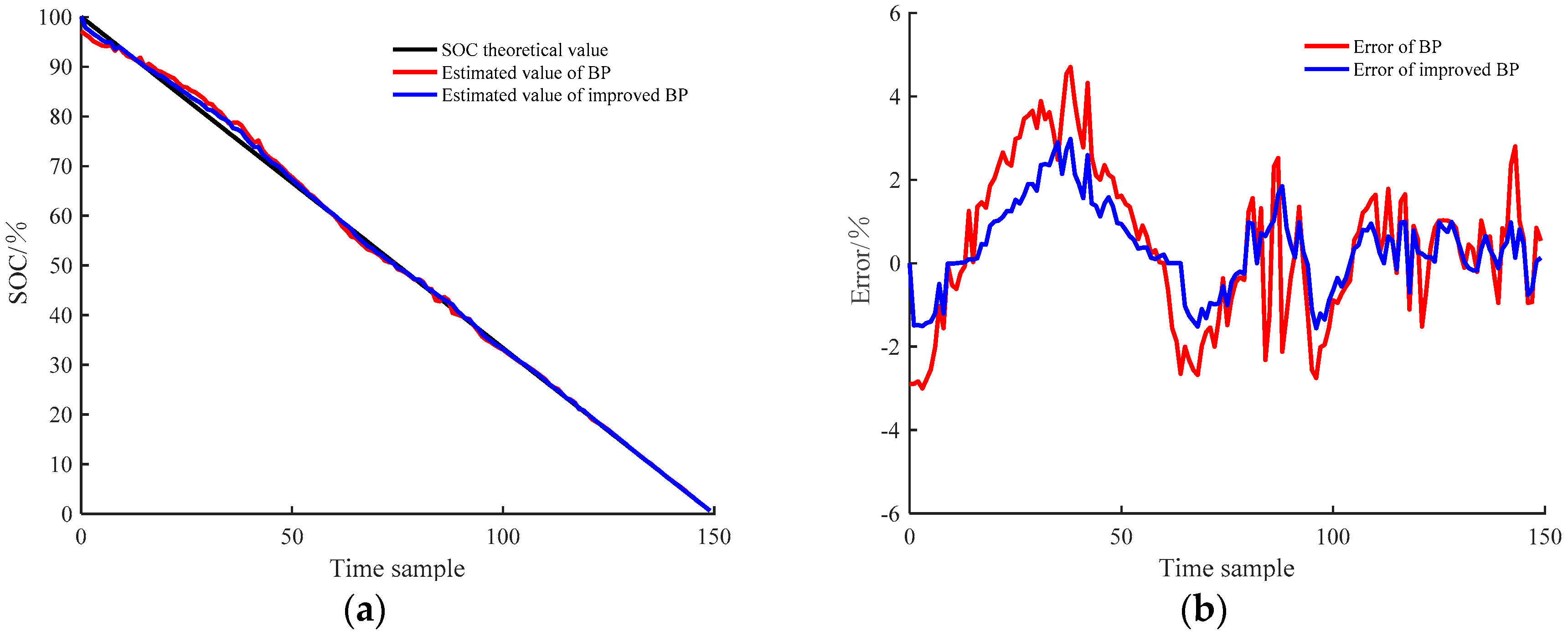
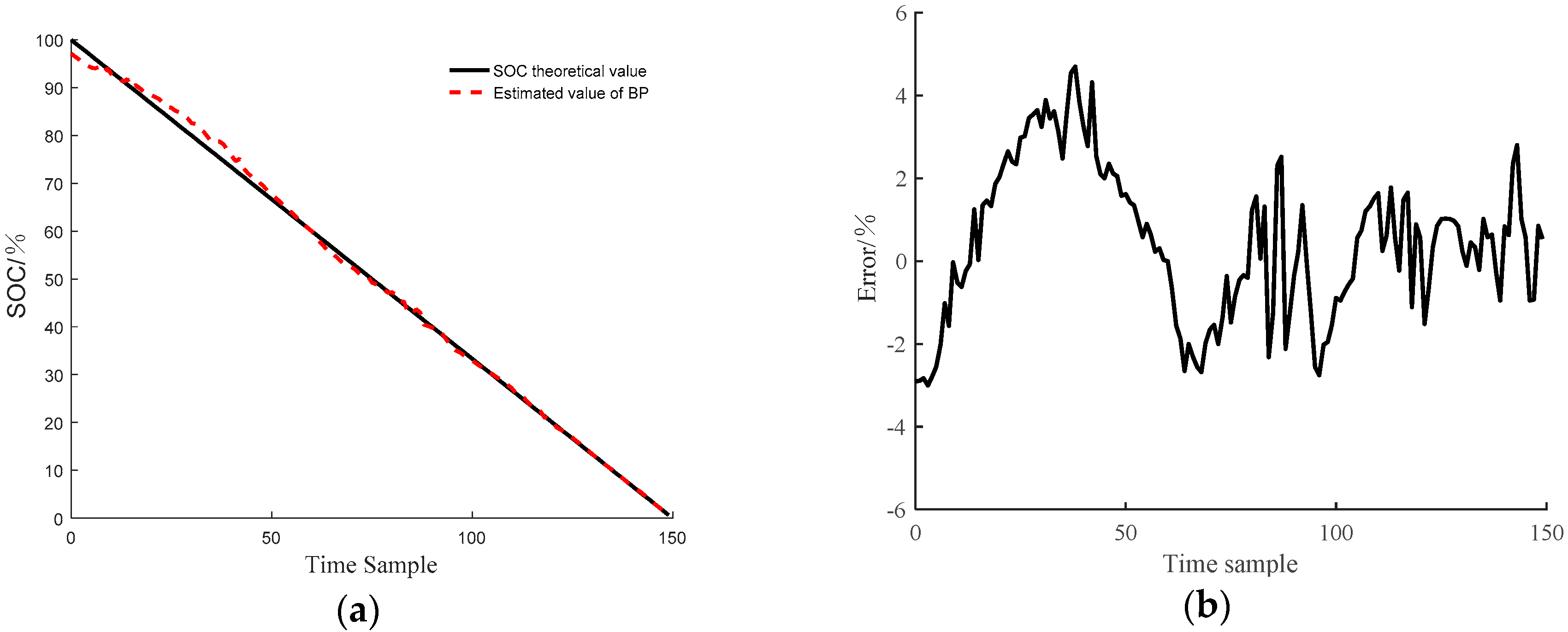
5.2. Back Propagation Neural Network Simulation

After the sample collection and selection process was completed, the normalized processing of the samples followed, thus accelerating the convergence speed of the network and improving the accuracy of the network. The data were then imported into the neural network model for training. First, the neural network model needed to be initialized. Next, the corresponding maximum number of iterations, target mean square error, learning rate, and initial weight were set. Then training could begin. After inputting the training samples, the model of the neural network was trained and adjusted based on the actual samples, until the mean square error (MSE) of the final output value and the theoretical output value met the needs of setting or the maximum number of iterations.
Through constant debugging and training, the key parameters of the network model were determined, as shown in Table 1.
After completing the training of the neural network, the next step is to complete the estimation accuracy of the neural network model. The 1500 group test samples were input into the neural network model that was completed by training, and the corresponding network output was obtained. Subsequently, the theoretical output was compared with the actual output of the network. The corresponding output is shown in Figure 6.
It can be seen from Figure 4 that the predicted value of the BP neural network model output after training is basically consistent with the theoretical prediction. By further analyzing the relative error comparison curves, it can be seen that the estimation error of the SOC is within 5%, which basically meets the requirements of SOC estimation in the industry. However, there is still room for further improvement.

5.3. Improved Back Propagation Neural Network Simulation

The data follows the training data and validation data of the previous model. Through continuous training, it was finally determined that when the training sequence reaches 320 steps, the mean square error reaches the minimum and meets the design requirements. Therefore, the same validation data were selected to verify the improved model. The corresponding SOC estimation effect is shown in Figure 7.
It can be seen from Figure 7 that the SOC estimation accuracy of the BP neural network algorithm is 2 percentage points higher than that of the traditional BP neural network algorithm. The total estimation error can be controlled within ±3% to meet the industry requirement of 5% error.

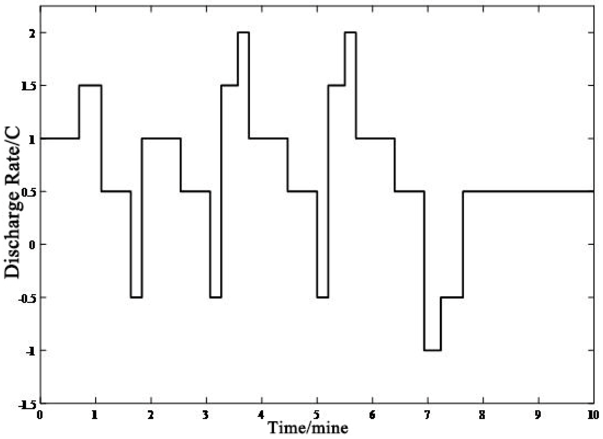
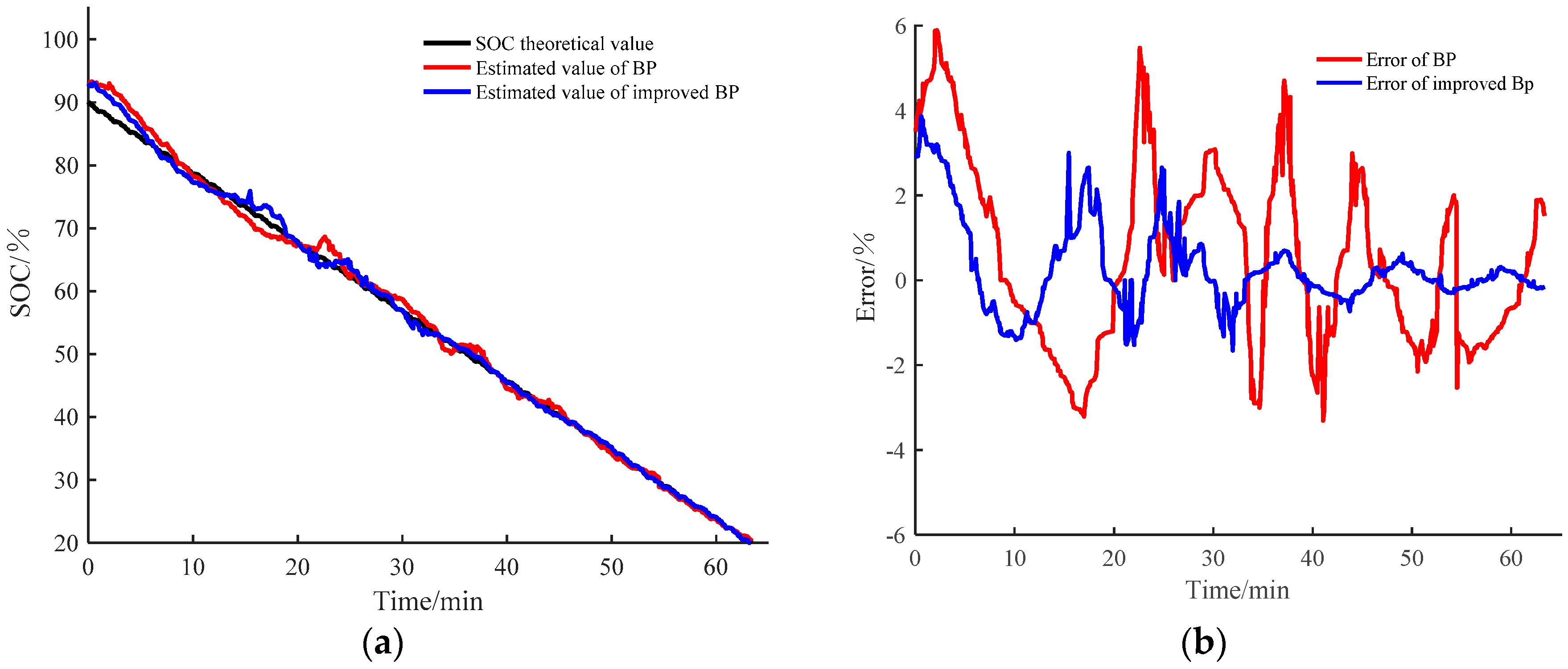
5.4. Working Condition Test

In order to verify whether the traditional BP neural network algorithm and the improved BP neural network algorithm can be applied to the actual operating conditions, the actual operating conditions were established in accordance with the special DST (Dynamic Stress Test) conditions for electric vehicle batteries. This simplified working condition model refers to DST working condition in the USABC (United States Advanced Battery Consortium) manual and the domestic battery testing manual, as shown in Figure 8.
According to the established model of real vehicle operation conditions, the cycle simulation of the operating condition was carried out using a charge and discharge tester until the power was exhausted. Then, the original data samples were collected and imported into the neural network model for training. After training, the condition test experiment was carried out. By receiving the corresponding voltage, current, temperature, and cycle times of the battery, the two neural networks output the estimated SOC value, and the corresponding estimated SOC relative error of the two algorithms is shown in Figure 9.
It can be seen from Figure 9a that as the discharge progresses, the error of the two improved algorithms becomes increasingly smaller. However, in Figure 9b we can see that the SOC estimation error of the unimproved neural network algorithm reaches 6%, indicating poor performance under actual working conditions. Meanwhile, the improved neural network algorithm can accurately estimate the SOC value of the battery under practical conditions, and the estimated error can be controlled within 4%. The accuracy of estimation is slightly lower than that under the condition of constant multiple discharge, as shown in Figure 7, but it can meet the industry requirement of less than 5% error, which has certain guiding significance.

6. Conclusions

Based on the advantages and disadvantages of the mainstream SOC estimation algorithm and the problem of power battery SOC estimation, a kind of SOC estimation algorithm based on BP neural network was proposed in this paper. Furthermore, the SOC estimation model based on BP neural network was established. At the same time, because the BP neural network is prone to falling into the extreme local minimum due to the defects of its own optimization algorithm, a new neural network algorithm was proposed to realize SOC estimation using an improved and optimized neural network model. Matlab was used to verify the estimation accuracy of the two algorithms, and the comparison results are shown in Table 2. The results show that the estimation error of the neural network algorithm is less than 3%, which satisfies the industry requirement of a maximum of 5% error.
To verify whether the improved algorithm can be used in actual operating conditions, real vehicle working conditions based on a DST model were established and the working condition data were imported into the improved neural network for training. The experimental results show that the improved BP neural network control algorithm can meet the SOC estimation of a power battery under actual operating conditions, and the error was controlled within 4%. The accuracy of SOC estimation error of the optimized network model was improved by 2 percentage points, which has a certain value for the promotion of this model.

Author Contributions

Conceptualization, C.-W.Z.; Data curation, S.-R.C.; Formal analysis, K.-J.X.; Investigation, H.-B.G.; Software, M.-Y.Y.

Acknowledgments

This work was supported by the National Key R&D Program of China (2018YFC0808203). It was also financially supported by the Xi’an University of Science and Technology.

Conflicts of Interest

The authors declare no conflict of interest.

Nomenclature

BMSBattery management system
SOCState of charge
BPBack propagation
DVDifferential voltage
EKFExtend Kalman filter
PFParticle filter
OCVOpen circuit voltage
PSOParticle swarm optimization
MSEMean square error
LMLevenberg Marquardt
CCCVConstant current constant voltage
DSTDynamic Stress Test
USABCUnited States Advanced Battery Consortium
PiOutput of the hidden layer
YkOutput of the output layer
pTransfer function of the hidden layer
qTransfer function of the output layer
ωijConnection weight between the input layer and the hidden layer
ωjkConnection weight between the hidden layer and the output layer
MNumber of input layers
LNumber of hidden layers
NNumber of output layers
XVector of input variables
θThreshold value
EMean square error
tkExpected output
YkActual output
ωaCurrent state weight
ηLearning rate
mNumber of input layer nodes
aAdjustment coefficient

References

  1. Safari, M. Battery electric vehicles: Looking behind to move forward. Energy Policy 2018, 115, 54–65. [Google Scholar] [CrossRef]
  2. Jenn, A.; Springel, K.; Gopal, A.R. Effectiveness of electric vehicle incentives in the United States. Energy Policy 2018, 119, 349–356. [Google Scholar] [CrossRef]
  3. Kumar, B.; Khare, N.; Chaturvedi, P.K. FPGA-based design of advanced BMS implementing SOC/SOH estimators. Microelectron. Reliab. 2018, 84, 66–74. [Google Scholar] [CrossRef]
  4. Nembrini, J.; Évéquoz, F.; Baeriswyl, R.; Lalanne, D. Advocating the use of visual analytics in the context of BMS data open access. Energy Procedia 2017, 122, 715–720. [Google Scholar] [CrossRef]
  5. Xiong, R.; He, H.W.; Ding, Y. Study on identification approach of dynamic model parameters for lithium-ion batteries used in hybrid electric vehicles. J. Power Electron. 2011, 45, 100–104. [Google Scholar]
  6. Xiong, R.; He, H.W.; Sun, F.C.; Zhao, K. Evaluation on state of charge estimation of batteries with adaptive extended Kalman filter by experiment approach. IEEE Trans. Veh. Technol. 2013, 62, 108–117. [Google Scholar] [CrossRef]
  7. Awadallah, M.A.; Venkatesh, B. Accuracy improvement of SOC estimation in lithium-ion batteries. J. Energy Storage 2016, 6, 95–104. [Google Scholar] [CrossRef]
  8. Wu, T.; Wang, M.; Xiao, Q. The SOC estimation of power li-ion battery based on ANFIS model. Smart Grid Renew. Energy 2012, 3, 51–55. [Google Scholar] [CrossRef]
  9. Hannan, M.A.; Lipu, M.S.H.; Hussain, A.; Mohamed, A. A review of lithium-ion battery state of charge estimation and management system in electric vehicle applications: Challenges and recommendations. Renew. Sustain. Energy Rev. 2017, 78, 834–854. [Google Scholar] [CrossRef]
  10. Huang, S.C.; Tseng, K.H.; Liang, J.W. An online SOC and SOH estimation model for lithium-ion batteries. Energies 2017, 10, 512. [Google Scholar] [CrossRef]
  11. Peng, S.; Zhu, X.L. An adaptive state of charge estimation approach for lithium-ion series-connected battery system. J. Power Sources 2018, 392, 48–59. [Google Scholar] [CrossRef]
  12. Zheng, F.D.; Xing, Y.J.; Jiang, J.C.; Sun, B.X. Influence of different open circuit voltage tests on state of charge online estimation for lithium-ion batteries. Appl. Energy 2016, 183, 513–525. [Google Scholar] [CrossRef]
  13. Dang, X.J.; Yan, L.; Xu, K. Open-circuit voltage-Based state of charge estimation of Lithium-ion battery using dual neural network fusion battery model. Electrochim. Acta 2016, 188, 356–366. [Google Scholar] [CrossRef]
  14. Yang, N.X.; Zhang, X.; Li, G. State of charge estimation for pulse discharge of a LiFePO4 battery by a revised Ah counting. Electrochim. Acta 2015, 151, 63–71. [Google Scholar] [CrossRef]
  15. Xu, D.P.; Wang, L.F.; Yang, J. Research on Li-ion battery management system. In Proceedings of the 2010 International Conference on Electrical and Control Engineering, Wuhan, China, 25–27 June 2010. [Google Scholar]
  16. Baba, A.; Adachi, S. State of charge estimation of HEV/EV battery with series Kalman filter. In Proceedings of the 2012 Proceedings of SICE Annual Conference (SICE), Akita, Japan, 20–23 August 2012; pp. 845–850. [Google Scholar]
  17. Zheng, L.F.; Zhu, J.G. Differential voltage analysis based state of charge estimation methods for lithium-ion batteries using extended Kalman filter and particle filter. Energy 2018, 158, 1028–1037. [Google Scholar] [CrossRef]
  18. Guo, Y.F.; Zhao, Z.S.; Huang, L.M. SOC Estimation of lithium battery based on improved BP neural network. Energy Procedia 2017, 105, 4153–4158. [Google Scholar] [CrossRef]
  19. Posewsky, T.; Ziener, D. Throughput optimizations for FPGA-based deep neural network inference. Microprocess. Microsyst. 2018, 60, 151–161. [Google Scholar] [CrossRef]
  20. Pan, H.H.; Lu, Z.Q.; Lin, W.L.; Li, J.Z.; Chen, L. State of charge estimation of lithium-ion batteries using a grey extended Kalman filter and a novel open-circuit voltage model. Energy 2017, 138, 764–775. [Google Scholar] [CrossRef]
  21. Li, Z.; Lu, L.G.; Ou, Y. The method of evaluating the accuracy of battery SOC is compared by improving the Ann time integral method. J. Tsinghua Univ. (Nat. Sci.) 2010, 50, 1293–1296. [Google Scholar]
  22. Mao, H.F.; Wan, G.C.; Wang, L.; Zhang, Q. Battery SOC estimation based on Kalman filter correction algorithm. Chin. J. Power Sources 2014, 38, 298–302. [Google Scholar]
  23. Afshar, S.; Morris, K.; Khajepour, A. State of charge estimation via extended Kalman filter designed for electrochemical equations. IFAC PapersOnLine 2017, 50, 2152–2157. [Google Scholar] [CrossRef]
  24. Xiang, Y.; Liu, C.G.; Su, J.Q.; Yang, G.B. Forecast model of battery state of charge based on BP network and its optimization. Chin. J. Power Sources 2013, 137, 963–965. [Google Scholar]
  25. He, W.; Williard, N.; Chen, C.C.; Pecht, M. State of charge estimation for Li-ion batteries using neural network modeling and unscented Kalman filter-based error cancellation. J. Electr. Power Energy Syst. 2014, 62, 783–791. [Google Scholar] [CrossRef]
  26. Feng, J. BP neural network predicts the selection of SOC training data for li-ion battery. Chin. J. Power Sources 2016, 140, 283–286. [Google Scholar]
  27. Panchal, S.; Dincer, I.; Agelin-Chaab, M.; Fraser, R.; Fowler, M. Experimental and theoretical investigation of temperature distributions in a prismatic lithium-ion battery. Int. J. Therm. Sci. 2016, 99, 204–212. [Google Scholar] [CrossRef]
  28. Panchal, S.; Dincer, I.; Agelin-Chaab, M.; Fraser, R.; Fowler, M. Thermal modeling and validation of temperature distributions in a prismatic lithium-ion battery at different discharge rates and varying boundary conditions. Appl. Therm. Eng. 2016, 96, 190–199. [Google Scholar] [CrossRef]
Figure 1. Back propagation neural network three-layer model.
Batteries 04 00069 g001
Figure 2. Improved algorithm weight adjustment schematic diagram.
Batteries 04 00069 g002
Figure 3. Training sample collection.
Batteries 04 00069 g003
Figure 4. Back propagation (BP) neural network improvement algorithm.
Batteries 04 00069 g004
Figure 5. Data acquisition platform (the battery is in thermostat).
Batteries 04 00069 g005
Figure 6. BP network estimation accuracy: (a) Comparison curves between SOC estimation and theoretical values; (b) the error curves of the estimation methods compared with the theoretical values.
Batteries 04 00069 g006
Figure 7. The estimation accuracy of the state of charge (SOC) before and after the algorithm is improved: (a) Comparison curves between different estimation methods and SOC theoretical values; (b) the error curves of the two estimation methods compared with the theoretical values.
Batteries 04 00069 g007
Figure 8. Simulated working conditions.
Batteries 04 00069 g008
Figure 9. SOC comparison diagram of working condition experiment: (a) Comparison curves between different estimation methods and SOC theoretical values; (b) the error curves of the two estimation methods compared with the theoretical values.
Batteries 04 00069 g009
Table 1. Key parameters of the network model.
Network ParametersValueNetwork ParametersValue
Maximum number of iterations1000Learning rate0.05
Target mean square error4–10Optimal number of iterations312
Table 2. Error comparison of the simulation analysis by different methods.
Research MethodsBP Neural NetworkImproved BP Neural Network
Maximum estimation error in simulation5%3%
Maximum estimation error in working condition test6%4%

