Advanced Load Cycle Generation for Electrical Energy Storage Systems Using Gradient Random Pulse Method and Information Maximising-Recurrent Conditional Generative Adversarial Networks ^†

Abstract

The paper presents two approaches to generating load cycles for electrical energy storage systems. A load cycle is described as the operation of an energy storage system. The cycles can include different metrics depending on the storage application. Load cycle analysis using the rainflow counting method is employed to understand and validate the metrics of the load cycles generated. Current load cycle generation can involve clustering methods, random microtrip methods, and machine learning techniques. The study includes a random microtrip method that utilises the Random Pulse Method (RPM) and enhances it to develop an improved version called the Gradient Random Pulse Method (gradRPM), which includes the control of stress factors such as the gradient of the state of charge (SOC). This method is relatively simple but, in many cases, it fulfills its purpose. Another more sophisticated method to control stress factors has been proposed, namely the Information Maximising-Recurrent Conditional Generative Adversarial Network (Info-RCGAN). It uses a deep learning algorithm to follow a machine learning-based, data-driven load cycle generation approach. Both approaches use the measurement dataset of a BMW i3 over multiple years to generate new synthetic load cycles. After generating the load cycles using both approaches, they are applied in a laboratory environment to evaluate the stress factors and validate how similar the synthetic data are to a real measurement. The results provide insights into generating simulation or testing data for electrical energy storage applications.

1. Introduction

The number of electrical energy storage applications has increased significantly in recent years. The push for electric vehicles and stationary systems is enormous. No matter which application the electrical energy storage system is used for, significant effort is put into improving the system’s control and enhancing the understanding of the application and its requirements. For this purpose, the systems are either tested in laboratories, applying different load cycles, or simulated. Either approach requires adequate knowledge of the system’s requirements and behaviours during the application. Furthermore, the appropriate input data are required to represent the given application’s stress factors. Recent research by Ref. [1] showed that a varying dynamic discharge profile led to an increase of up to 38% in equivalent full cycles at the end of life. In Ref. [2], differences in the degradation were recorded, especially for low temperatures. A review of battery data in Ref. [3] revealed that dynamic ageing has often been overlooked in degradation analysis, primarily due to the complexity of assessing ageing mechanisms under dynamic stress factors and the limited availability of real-world application data for dynamic cycles. Additionally, degradation studies are frequently accelerated to reduce time and effort. This underscores the usefulness and necessity of load cycle generation approaches. This work shows an approach to extracting the required information from measurements and using them to generate new (simplified) load cycles through load cycle analysis. Two different methods for load cycle generation are introduced and compared. This work is developed based on our preliminary work [4], upon which the content is significantly expanded. The expansion includes the tuning of the two methods introduced and makes it possible to compare the approaches based on their influences on actual laboratory measurements instead of relying on comparing synthetically generated load cycles. In particular, the influence of gradRPM on secondary stress factors, such as temperature and voltage, can be evaluated and validated through the Info-RCGAN approach. The preliminary work does not include any validation in a laboratory environment.

Load cycle analysis is necessary to evaluate the data, identify the relevant stress factors to design a degradation schedul, and validate the load cycles generated. Different approaches can be found in the literature. Ref. [5] summarised papers utilising various approaches to load spectrum analysis. The methods included instantaneous value counting, rainflow counting, range pair mean counting, total charge throughput, and half-cycle counting. The techniques can be used for different stress factors. Instantaneous value counting is a method where the appearance of each value belongs to a bin, and the specific bin counter is incremented. Every value is counted. Charge throughput calculates the charge that is charged or discharged instead of occurrences. The occurrences do not include varying sample times. Rainflow counting is more complex and counts stress cycles and their mean values and ranges. Rainflow counting can be applied to different stress factors such as SOC, temperature, voltage, and current. The results can be displayed as histograms or spectra. In Ref. [6], the rainflow counting was extended using a fuzzy logic approach to address the quantisation error implicit in the histogram generation that could have introduced incorrect representations of the stress signal. In addition, it has been used as the basis for battery degradation models to account for temperature and c-rate dynamics, such as in Ref. [7]. Ref. [8] highlighted the drawbacks of applying rainflow counting to real-time data and introduced a faster method to approximate the full cycles that a battery endured during a frequency response application. In Ref. [9], the problem of applying the rainflow counting approach to real-time data, as well as in an optimisation problem, was addressed by counting the half cycles generated by each concavity change. In Ref. [10], machine learning approaches were applied to analyse the stress factors and rank them. The least absolute shrinkage and selection operator was used for the analysis, and a random forest approach was employed to perform the ranking. In general, variations of the rainflow counting method have been widely used as approaches to stress analysis. This method breaks down complex load cycles into stress cycles, capturing the range and mean of each cycle. It can easily be applied to multiple stress factors that are critical for battery degradation processes, such as state of charge, temperature, voltage, and current. Its representation through histograms or spectra is explicitly useful for the easy comparison and interpretation of measurement data and the load cycles generated. Due to its versatility, rainflow counting is used in this work for the analysis of the profiles generated and the investigation of the stress factors of the measurement data.

Load cycle generation is often described using driving cycles. In the case of driving cycles, vehicle kinematics are used to design cycles, which are then run with a simulation. Afterwards, a battery profile can be calculated. Load cycles generally pertain to the load profile applied to batteries and battery systems. The literature concerning load cycles is sparse, whereas there is more literature using different approaches for driving cycles. Nevertheless, approaches to driving cycle construction can be used for load cycle generation. In general, cycle generation can be divided into three different categories. Simple methods based on employing known profiles to generate new variations using, for example, battery models or vehicle models. In Ref. [11], a battery model was used to generate the synthetic data of an end-of-line test, which was then used to train a machine learning algorithm. Clustering methods can be used to help identify features and categorise measurement data to reduce the data information to a single drive cycle like a standard drive cycle, i.e., the New European Driving Cycle (NEDC). In Ref. [12], principal component analysis, clustering, and an optimisation algorithm were used to obtain a driving cycle that was typical for the data acquired during the case study, whereas in Ref. [13], a relatively raw clustering approach used principal component analysis to reduce the dimensionality, as well as clustering to categorise the microtrips. Afterwards, the microtrips were randomly picked to construct a new cycle. Random microtrip methods include restructuring the measurement data randomly to new cycles, like in Ref. [14]. In Ref. [15], the generation of a load cycle for electrical vehicle application was based on the data from a real electrical vehicle, where different methods were used to classify the uses of the vehicle, including, for example, K-Means clustering; the dimensionality of the features was reduced using principal component analysis. For the characterisation of driving cycles in Ref. [16], the energy consumption per unit of time was used as an indicator to classify the cycles into semi-urban or semi-highway cycles. The categories were characterised, and probability functions were designed to represent the categories. Afterwards, the functions were sampled with a random seed to generate new profiles. In Ref. [17], cycles were generated for a stationary application. The data were divided into intervals, and twelve different metrics were calculated to describe the intervals. A dispatch interval matrix was designed for further analysis. Principal component analysis was used to reduce the dimensions before unsupervised K-Means clustering was applied for the categorisation. For the cycle generation, a number of characteristic duty cycles were extracted. Other approaches include machine learning methods. Sometimes, they are used to improve the existing clustering methods. In Ref. [18], an autoencoder was added to the clustering method to improve the generation of a new cycle by half a percent, whereas in Ref. [19], a Time Generative Adversarial Network was applied to generate more synthetic data on different driving conditions and operational parameters like varying temperatures for the training of a state of charge prediction model. So, there are multiple approaches to generating usable load cycles, from simple to advanced. To reach the goal of creating realistic controllable load cycles for application in a laboratory environment, two approaches are implemented during this study. The first approach belongs to the group of approaches that reuses segments of the original measurement data. The simple algorithm is based on the RPM from Ref. [14] and was chosen as one of the approaches due to its ease of implementation, low requirements for computational resources, and the amount of data needed to generate adequate cycles. These advantages make the RPM a good candidate for straightforward load cycle generation. Expanding the RPM to include the possibility of controlling different stress factors leads to the development of the gradRPM. However, not all of the stress factors can be controlled by the gradRPM; to do so, a parameterised battery model would be needed to model the voltage and temperature responses to the generated load cycle. That would increase the complexity and information needed to generate load cycles, which is not part of this work for the gradRPM. The second approach is aimed at using the Info-RCGAN. The Info-RCGAN is used to generate load cycles that resemble the measurement data as much as possible, with advanced stress factor control for secondary stress factors such as temperature and voltage. Using a large dataset for training increases adaptability and flexibility. Furthermore, this approach is able to capture more complex dependencies between the stress factors than a simple approach. These advantages make it a perfect cross-comparison for the gradRPM method. Both approaches need a real-world measurement dataset, where the amount of data may vary. The gradRPM can work even using just a small amount of data, where the Info-RCGAN needs a larger amount to effectively train the whole model. By combining a simpler, computationally efficient method (gradRPM) with an advanced, high-fidelity approach (Info-RCGAN), we aim to provide a more comprehensive solution for load cycle generation. These methods are tested using real-world data from a BMW i3 and validated in a laboratory environment.

The paper is structured as follows: First, we describe the dataset used as a reference and the basis of our study, see Section 2. Next, we present the methodology, which is divided into two approaches, the gradRPM in Section 3.1 and the Info-RCGAN in Section 3.3. This is followed by the results of the two approaches and a discussion of the findings in Section 4. Finally, we conclude the paper with key insights and implications in Section 5 and Section 6.

2. Dataset

The dataset used as the basis for this data-driven pulse generation comprises logged data from a BMW i3 (BMW AG, Munich, Germany). It includes data recorded over 4 years, with shorter trips in most cases. The BMW i3 belongs to the Fraunhofer Institute for Transportation and Infrastructure Systems (Dresden, Germany) and is regularly used as a passenger car. Consequently, the gathered data closely resemble the driving patterns of a private BMW i3 owner. Figure 1 displays a summary of the dataset for the range of SOC per trip, its mean SOC, and the mean temperature. The colours, starting from yellow to violet, in the scatter plot indicate the time of acquisition, where yellow is the oldest measurement, i.e., the cell had a higher SOH at this point. In general, the trips are shorter, with an SOC range of up to 20%, and they mostly cycled around an SOC of 75%, which is rather high. Over the ageing of the battery, the mean SOC decreases. The temperature typically remains between 20 °C and 30 °C, with brief deviations occurring only at cold or hot ambient temperatures immediately after vehicle startup. Therefore, the temperature is not displayed here. Each measurement includes voltage, current, SOC, time and temperature. The Fraunhofer Institute for Transportation and Infrastructure Systems provided the data for the joint research project “Field Data-Based Battery Diagnosis and Lifetime Prediction (FeBaL)”. The project goal was the utilisation of field data to improve battery assessment by learning the ageing behaviour, including stress factors and interactions, examining the ageing without a capacity test, and understanding the usage patterns for application-specific lifetime predictions.

3. Methodology

The methodology is subdivided into three different parts. Load cycle analysis is the first part, the improved random pulse method is the second, and the third is the machine learning-based approach to cycle generation. To compare and validate the generation of the profiles with the measurements, there needs to be a way of analysing the profiles generated. Some approaches have been mentioned in Section 1. In this work, the rainflow counting method is used to analyse all the generated and measurement data concerning the stress factors, SOC, temperature, voltage, and current or C-rate. Regarding the generation, the only analysable factor is the C-rate because, for example, the RPM (Section 3.1) only generates a C-rate profile. On the other hand, the machine learning approach (Section 3.3) can generate profiles for the different stress factors, but in the end, only the C-rate profile is applied.

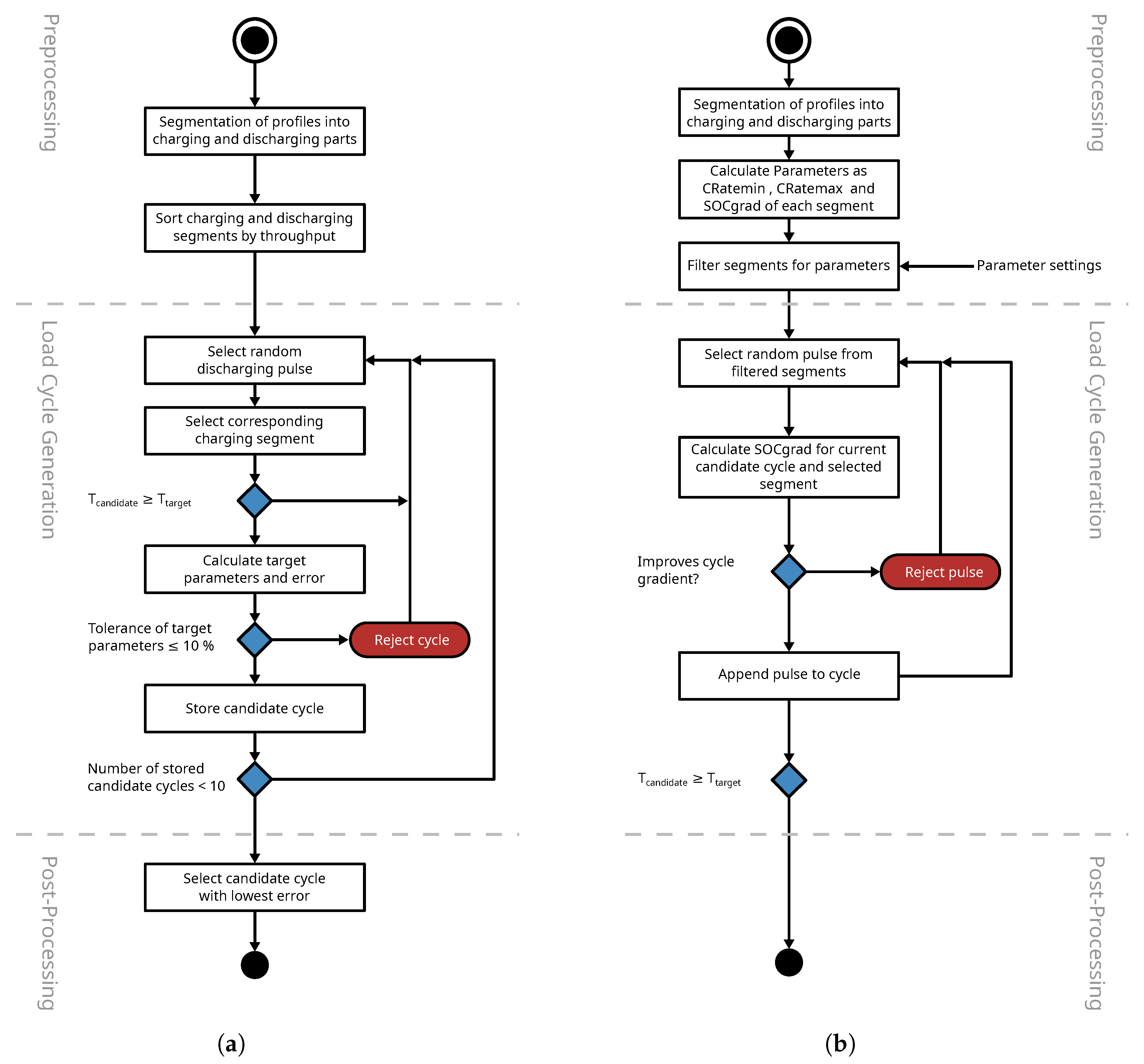
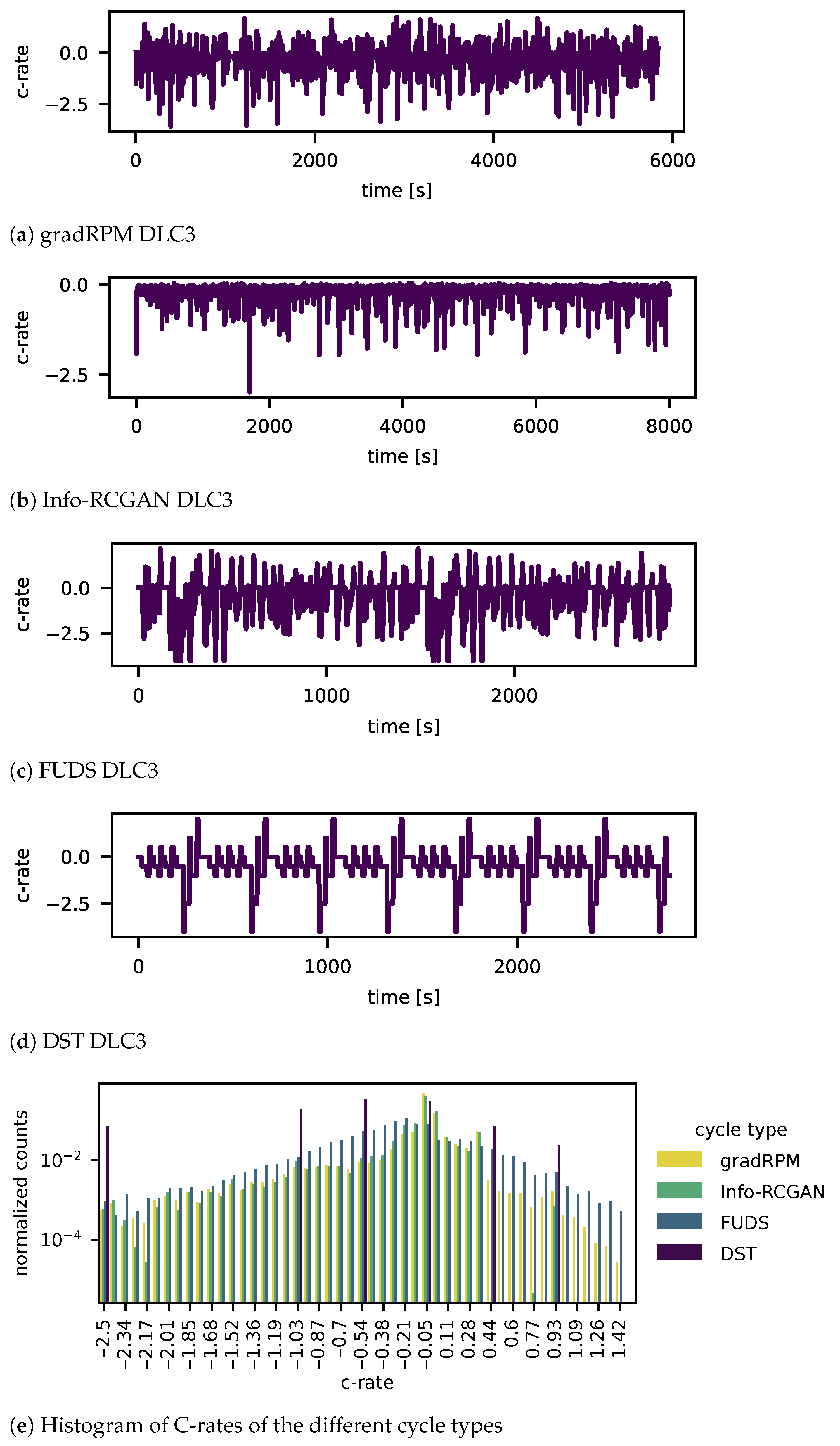
3.1. Gradient Random Pulse Method (gradRPM)

The Random Pulse Method (RPM) is highly dependent on the measurements and the number of measurements within the dataset used to extract information on the application. In Ref. [14], the method was introduced to construct driving schedules for high-performance batteries used in racing applications on specified racing tracks. Ref. [14] described segmenting the dataset into smaller parts of the dataset. A segment’s start and end were defined by the current direction change, either from the discharging to the charging direction or vice versa. Therefore, the data were analysed for zero crossings and split into segments. The segments were then saved to a database, and the charging and discharging databases were subdivided. Furthermore, the databases could be arranged into racetrack-specific segments. Then, the databases were analysed considering predefined target parameters, where applicable. The target parameters described different characteristics of the data. They included the mean power discharge and charge, as well as the mean absolute power and net discharge power. In addition, they considered parameters describing the fraction of charging or discharging of the pulse. Different duration metrics were included in the target parameters and the overall duration. Some parameters were not calculated for the segments since they did not make sense, like the fraction of charging or discharging. Because of the segmentation, a segment was either a charging or discharging pulse. The target parameters were the criteria for the load cycles constructed to decide whether they were helpful. The databases of the charging and discharging segments were sorted by the duration of the segments. The generation of the profile used by Ref. [14] started with generating a random number within the range of the number of segments in the discharging database. The corresponding discharging and charging segments with similar durations were added to the cycle. The reason for adding both a discharging and charging segment with similar durations was to have real profiles and to avoid the occurrence of a short discharge pulse followed by a long charging pulse that may lead to overcharging. When the target duration for the duty cycle was reached, the cycle was evaluated in relation to the target parameters. The error of the target parameters had to be below 10% in the case of Ref. [14]. About 200 iterations were needed to generate 10 candidates using the 10% margin [14]. The cycle was stored as a candidate if the target parameters were within the intended range. The procedure was repeated until ten candidates were stored. The overall error for each candidate was calculated, and the candidate with the lowest error was accepted. The general approach of the RPM is displayed in Figure 2a.

Based on the explained method utilised by Ref. [14], the RPM was improved to reduce the number of iterations and enhance its controllability. This approach is called gradRPM, is based on the RPM, and is tested in this paper. Controllability is especially important to generate load cycles that are used for dynamic ageing in laboratories. Because in ageing tests, the degradation is planned for specific stress factors. The stress factors that are investigated include the SOC range, the mean SOC or mean voltage, and the current rates for cyclic degradation. Target parameters and control parameters are used to control the stress factors. A minimum and maximum C-rate is included to maintain at least the boundaries of the current rates. Furthermore, an SOC gradient and range are part of the parameters used to control the mean SOC and range. The target parameters include the SOC range, that describes the maximum change of the SOC over the load cycle and the maximum duration of the load cycle.

The parameters are distinguished into control and target parameters because the process of the RPM has been altered. The new process of the SOC gradient-oriented RPM starts with filtering the database for pulses that are within the boundaries given by the parameters $CRat{e}_{\max }$, $CRat{e}_{\min }$ and within ±5% of $SO{C}_{\mathrm{gradient}}$. The information concerning the control parameters was already calculated when the segmentation of the actual data was performed, and they were saved to the pulse database as additional information, which is helpful for the generation of the load cycle. The database filtering reduces the pulses to usable ones to generate the load cycle for the given parameters. Then, a random number is generated in the range of the filtered database. A single segment is chosen. The segment could either be in the charge or in the discharge direction. The SOC gradient is calculated for the current load cycle and extracted from the database’s chosen segment. If the current gradient of the load cycle differs from the control parameter, only a segment that improves the gradient in the direction of the control parameter is accepted.Therefore, the resulting cycle has a gradient around the set SOC gradient by construction. The generation is finished if the candidate load cycle exceeds the requested SOC range or duration. The process of the basic RPM utilised by Ref. [14] and the adapted gradient-based approach are depicted in Figure 2.

The described approach of the gradRPM can generate more complex gradients as long as the database provides the required data. So, complex load cycles containing multiple segments with different SOC gradients can be generated by providing a sequence of parameters. An example is displayed in Figure 3. As expected, the higher the gradient, the higher the number of pulses with higher currents that reach the desired gradient for the load cycle.

3.2. Process of Analysing Dynamic Load Cycles

The analyses of dynamic data and actual driving data are carried out through the following steps:

• Preprocessing,
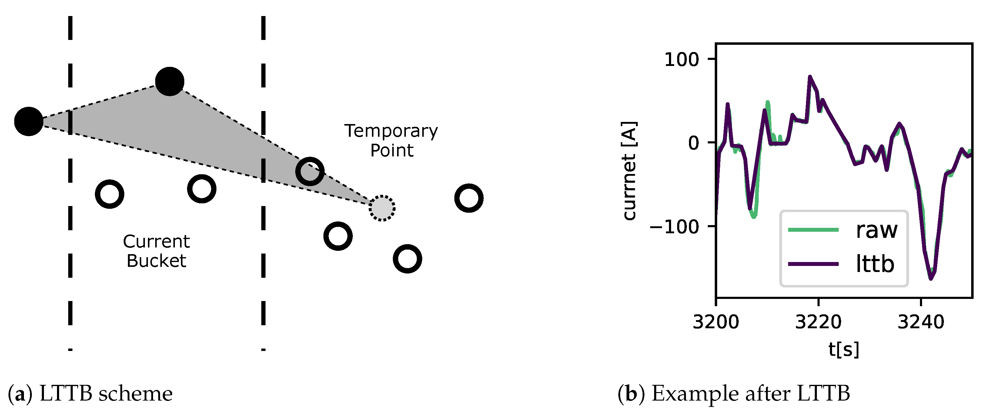
• Downsampling,
• And the analysis.

Preprocessing manages the analysis’ noise, outliers, and unimportant segments. Unimportant segments can be, in the case of a driving schedule, a prolonged time of data logging after the car is parked. In this work, another approach is used, combining preprocessing and downsampling. A unique sampling approach, a so-called importance sampling method, is used. In this specific case, it is the Largest-Triangle-Three-Bucket approach (LTTB). The reason for the use of an importance sampling approach is, on the one hand, to reduce the amount of data and thus shorten the calculation time of the analysis and, on the other hand, not lose essential segments of the data, like the peaks and valleys. These peaks are significant in identifying the stress factors of the C-rate. The LTTB sampling refers to the use of a shifting window over the data that is meant for downsampling. It divides the window into three buckets containing a predefined number of samples. A sample is chosen for each centre bucket. For the right bucket, a temporary point is calculated as the mean of the samples in that bucket. The left bucket is the old centre bucket with a previously chosen sample. These three samples form a triangle, and the LTTB aims to maximise the area of this triangle by selecting the sample for the centre bucket accordingly. Afterwards, the window shifts for one bucket size. The schematic in Figure 4a visualises the steps of the LTTB approach [20]. By applying the LTTB to the BMW data, the data are compressed by a factor of 100.

After preprocessing using the LTTB, the data concerning the stress factors can be analysed. There are different approaches for evaluating the data. They are divided into the following two categories: one-parametric and multi-parametric analysis. One-parametric analysis investigates the signal for only one parameter, like the mean or peaks. Multi-parametric analysis investigates the signal, for example, for both the mean and the range, visualising more signal information. For example, there is instantaneous value counting, where the signal is segmented into specified bin sizes, and every value of the signal is assigned a bin so that it is counted, resulting in a histogram. If the signal is sampled with one specified frequency, each bin count represents the time spent in this stress factor. Multi-parametric approaches, in many cases, consider two parameters because of the ability to be visualised. An example is rainflow counting, which analyses the reversals of signals to identify the stress cycles. It counts the cycles and categorises them based on their mean and range, considering two parameters [5]. Sometimes, another similar approach is mentioned, half-cycle counting, which is, in fact, part of a typical implementation of rainflow counting because during rainflow counting, the signal is analysed for peaks and valleys, where a half cycle is from one valley to one peak or vice versa. This half cycle is also counted as a half cycle in typical rainflow counting. During this work, instantaneous value counting and rainflow counting are applied to analyse the load cycles generated and the measurement data.

3.3. Data-Driven Approach (Info-RCGAN)

A machine learning approach for the generation of battery load profiles considering multiple stress factors is proposed in this work. Not only are the generated load profiles of the model expected to have the same fundamental properties as the real ones, but certain features of the generated profiles can also be regulated through the model’s conditional input.

3.3.1. Data Preprocessing

The sampling period of the original data is $0.01$ s; however, the samples are usually not even, which means there could be no samples for a period that is longer than the sampling time. Sometimes, the device is also shut down for a longer time, during which the batteries are charged. In order to obtain independent load profiles, the load profiles that include long stand-by periods are segmented into separate profiles; otherwise, the increase in voltage, state of charge, and temperature will be considered as a part of the individual load profile. The segmented profiles are then interpolated. Downsampling is applied to improve the efficiency of the training, with a sampling rate of 1 Hz. Since different features have different scales, the input features are normalised into the same range. Research has also shown that data normalisation is able to improve the performance of various networks [21]. The normalisation approach applied is min–max normalisation, with the expected data range as [−1, 1]. The equation for the transformation is given in Ref. [22].

3.3.2. Sequence Processing

Recurrent Neural Networks (RNNs) [23] are commonly used for the processing of time series [24,25]. However, a vanilla RNN suffers from the problem of a vanishing gradient, which can be solved by the refined RNN model, Long Short-term Memory (LSTM) [26]. LSTM introduces a gate mechanism to control which information the LSTM units should remember and which information they should forget to learn the sequences’ long-term dependencies. Because of its strong capability to capture temporal features, it has become one of the most used architectures in time series analysis [27]. Therefore, LSTM is utilised as a basic unit for sequence processing in this work.

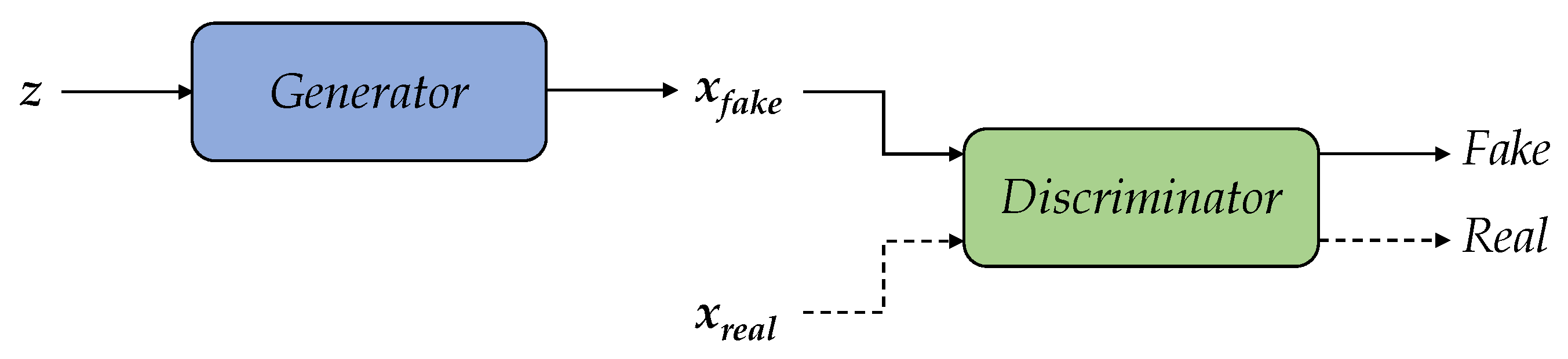
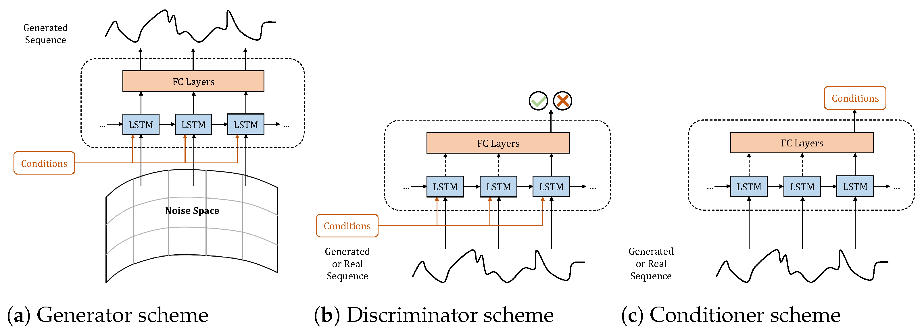
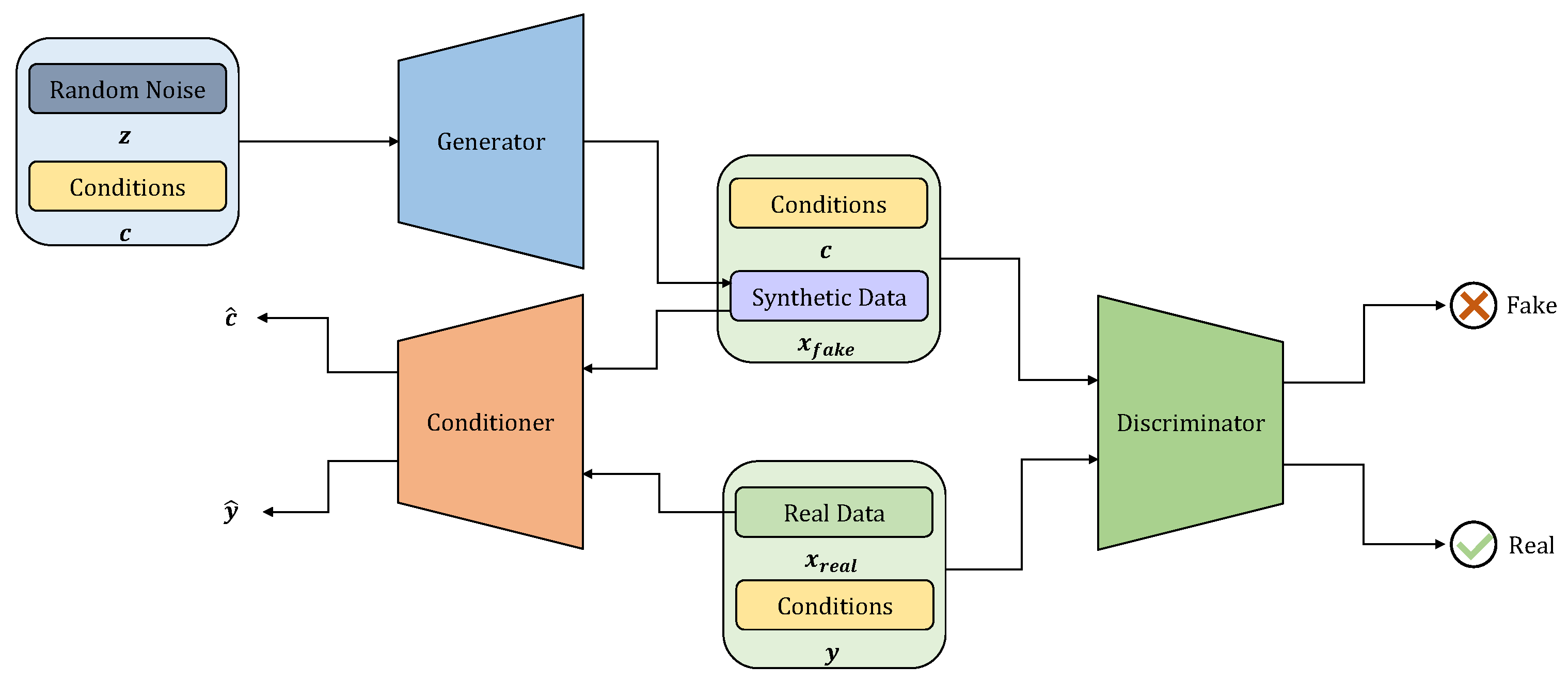
3.3.3. Generative Model

As one of the basic types of deep learning models, generative models aim to generate synthetic data by learning the data distribution throughout the space. In this work, a Generative Adversarial Network (GAN) [28] is utilised as the overall framework for load profile generation.

As shown in Figure 5, GAN consists of two components—the generator (G) and the discriminator (D). The generator takes random noise $\mathit{z}$ as input and produces synthetic data ${\mathit{x}}_{\mathrm{fake}}$. Given that the prior probability distribution of the input noise vector $\mathit{z}$ is $p_{\mathit{z}}\left(\mathit{z}\right)$, the generator aims to learn the distribution $p_g\left(\mathit{z}\right)$ such that its output resembles the ground truth data $\mathit{x}$. The transformation from noise space to data space is defined by the function $G(\mathit{z};{\theta }_g)$, in which G represents the generator’s neural network with the parameter ${\theta }_g$ [28]. The discriminator, on the other hand, receives either actual data ${\mathit{x}}_{\mathrm{real}}$ or fake data ${\mathit{x}}_{\mathrm{fake}}$ and outputs a probability indicating the likelihood that the input belongs to the ground truth. This mapping is represented by the function $D(\mathit{x};{\theta }_d)$, where D denotes the discriminator’s neural network with the parameter ${\theta }_d$ [28].

The generator and discriminator engage in a two-player minimax game and are jointly trained. The discriminator aims to maximise its accuracy in distinguishing between the real and generated data. In contrast, the generator aims to minimise the discriminator’s ability to identify the generated data as fake [28]. The value function $V(G,D)$ of the game is as follows:

$$\begin{array}{c}\hfill \underset{G}{\min }\underset{D}{\max }V(G,D)={\mathbb{E}}_{\mathit{x}\sim p_{\mathrm{data}}\left(\mathit{x}\right)}\left[logD\left(\mathit{x}\right)\right]+{\mathbb{E}}_{\mathit{z}\sim p_{\mathit{z}}\left(\mathit{z}\right)}\left[log(1-D\left(G\left(\mathit{z}\right)\right))\right]\end{array}$$

(1)

To incorporate conditional constraints into the load profile generation, the extended framework known as the Conditional Generative Adversarial Network (cGAN), introduced by Mehdi Mirza et al. [29], is utilised. In this framework, the naive GAN is modified to include conditional information $\mathit{y}$, which is provided as additional input to both the generator and discriminator. This conditioning information alters the value function of the two-player minimax game as follows:

$$\underset{G}{\min }\underset{D}{\max }V(G,D)={\mathbb{E}}_{\mathit{x}\sim p_{\mathrm{data}}\left(\mathit{x}\right)}\left[logD\left(\mathit{x}\right|\mathit{y})\right]+{\mathbb{E}}_{\mathit{z}\sim p_{\mathit{z}}\left(\mathit{z}\right)}\left[log(1-D\left(G\left(\mathit{z}\right|\mathit{y})\right))\right]$$

(2)

There are different approaches to embedding conditioning information into inputs, such as conditioning by concatenation [29], conditioning using an auxiliary classifier [30], and conditioning with projection [31]. After conducting several experiments, the conditioning approach by concatenation is chosen for this work. The inputs into the LSTM unit at each moment, both in the generator and the discriminator, are concatenated with the respective additional information.

The methods used in previous research, such as C-RNN-GAN [32] and RCGAN [33], have focused on generating continuous sequences using GANs by implementing the generator in a synchronous sequence-to-sequence manner [34]. In these models, the length of the generated sequence can be controlled by specifying the sequence length of the input noise. Building on this concept, Figure 6 illustrates the schematic diagrams of the generator and the discriminator. At each time step, the inputs into the LSTM unit in both the generator and the discriminator are concatenated with the corresponding additional information. To highlight the difference, the generator’s conditional input is denoted as $\mathit{c}$, while the actual data’s condition labels are denoted as $\mathit{y}$.

Most conditional GANs (cGANs) predominantly focus on categorical conditions [35]. In contrast, this work deals exclusively with continuous conditions, considerably complicating the learning process. Additional strategies are required to enhance learning outcomes. InfoGAN [36], initially designed for the unsupervised learning of disentangled representations, inspired the approach presented in this work. Specifically, the idea of strengthening the learning of additional information by integrating an auxiliary network and imposing extra penalties on condition reconstruction is adopted. By shifting the auxiliary model’s learning process to a supervised manner, controlling which specific information the auxiliary network extracts becomes possible. In this work, the auxiliary model is referred to as the conditioner. Its schematic diagram is depicted in Figure 7.

Figure 7 presents the overall architecture of the deep learning model utilised, Info-RCGAN. This work uses the following desired features as the conditional input $\mathit{c}$:

• $\Delta$SOC: the change in SOC after applying the load profile;
• $\Delta$T: the change in temperature of the battery pack;
• $min$(C-rate): the minimum C-rate within the load profile;
• $max$(C-rate): the maximum C-rate within the load profile;
• $min$($\Delta$U): the minimum voltage change throughout the load profile;
• $max$($\Delta$U): the maximum voltage change throughout the load profile.

Since validating desired features unrelated to the current on the dataset with a single generated C-rate output is challenging, the generated sequence is expanded to include three features: [C-rate, $\Delta$U, $\Delta$T]. This approach allows better insights into how temperature and voltage vary with the load profile under different conditional inputs.

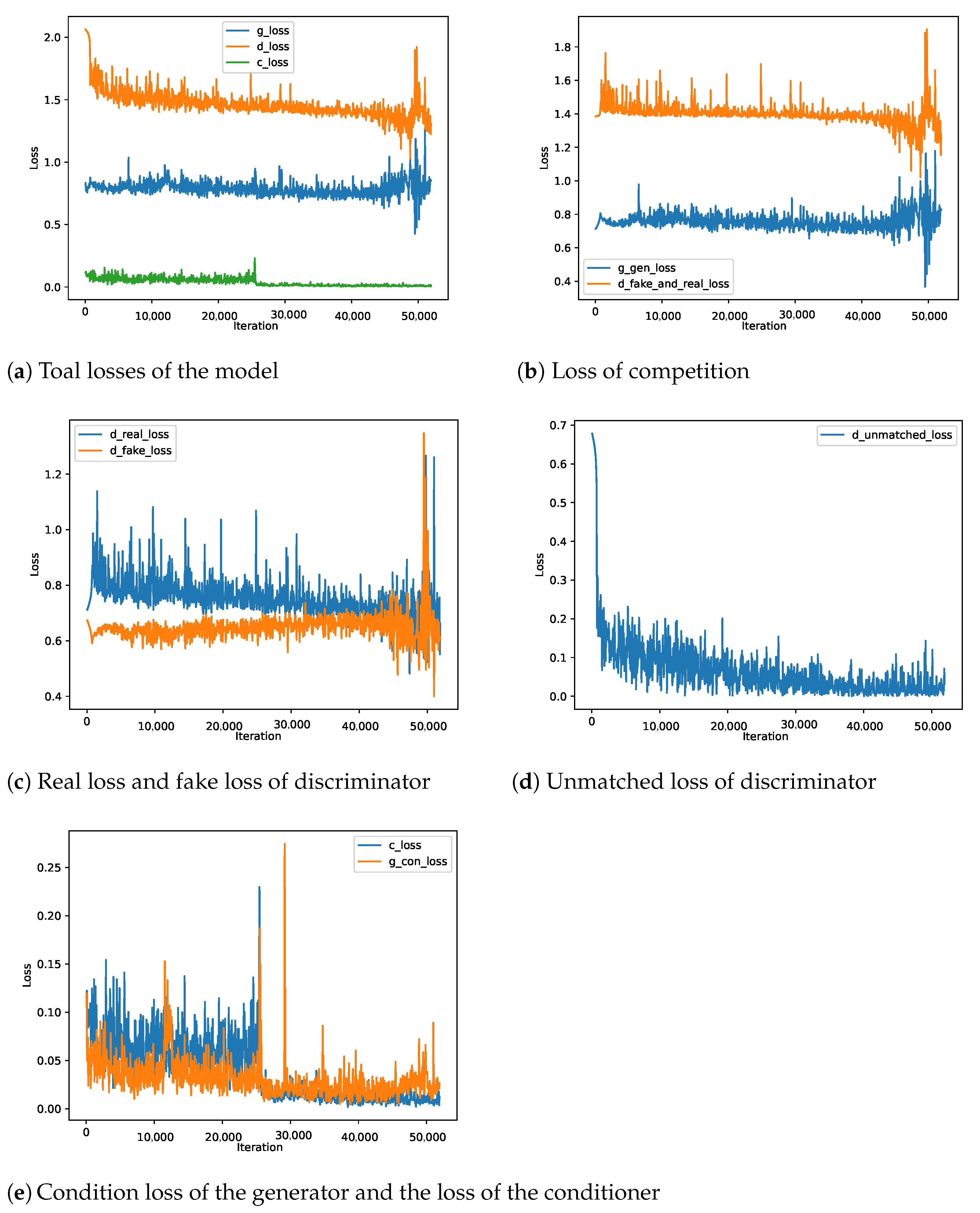
3.3.4. Loss Function Design

Since the architecture of the Info-RCGAN has multiple submodels, the proper design of loss functions also plays an essential role in this work. The loss functions that are used include Binary Cross Entropy (BCE) and Mean Squared Error (MSE).

The discriminator is expected to not only distinguish the generated fake data from the actual ground truth data but also to learn the condition information for distinguishing the different data types. To achieve this goal, the loss functions of the discriminator are as follows:

• Fake loss $BCE(D({\mathit{x}}_{\mathrm{fake}},\mathit{c}),\mathbf{0})$: to distinguish fake data with the respective conditional input as fake;
• Real loss $BCE(D({\mathit{x}}_{\mathrm{real}},{\mathit{y}}_{\mathrm{real}}),\mathbf{1})$: to distinguish real data with the respective real labels as real;
• Unmatched loss $BCE(D({\mathit{x}}_{\mathrm{real}},{\mathit{y}}_{\mathrm{fake}}),\mathbf{0})$: to distinguish real data with the unmatched labels as fake.

The following applies to the above-mentioned functions:

$${\mathit{x}}_{\mathrm{fake}}=G(\mathit{z},\mathit{c})$$

(3)

The conditioning input of the generator $\mathit{c}$ is chosen to be the ground truth labels ${\mathit{y}}_{\mathit{real}}$ from the same batch, and ${\mathit{y}}_{\mathit{fake}}$ are some randomly generated labels.

The conditioner aims to reconstruct the regression labels of the input sequence data. It is expected to learn specific desired features, as mentioned before, so the conditioner is trained on the ground truth data and its respective label in a supervised manner.

• Regression loss $MSE(C\left({\mathit{x}}_{\mathrm{real}}\right),{\mathit{y}}_{\mathrm{real}})$: to reconstruct the ground truth labels from the ground truth sequence data.

The generator is designed to achieve the following two goals: generate fake data that can fool the discriminator’s output into a “real” outcome, as well as generate data in which the condition input $\mathit{c}$ can be reconstructed by the conditioner. The loss functions used to train the generator are as follows:

• Generation loss $BCE(D({\mathit{x}}_{\mathrm{fake}},\mathit{c}),\mathbf{1})$: to generate data that can fool the discriminator;
• Condition loss $MSE(C\left({\mathit{x}}_{\mathrm{fake}}\right),\mathit{c})$: to generate data from which the input conditions can be reproduced by the conditioner.

The training of the generator is indirect performed through both the discriminator and the conditioner.

3.3.5. Training of the Model

GANs are notoriously difficult to train. We applied the hyperparameter optimisation framework Optuna [37] to search for the best learning rates for the generator, the discriminator, and the conditioner, respectively. Figure 8a shows the total training loss curves of the generator, the discriminator, and the conditioner. The training loss of the discriminator decreases rapidly in the beginning of the training process and then starts to decrease more gradually. The loss of the generator stays relatively steady throughout the whole training process. As for the conditioner, there is no obvious improvement in performance in the first half of the training; in contrast, the loss value drops significantly and stays stable at a low level in the second half of training.

Figure 8b shows the loss values directly related to the competition between the generator and the discriminator, namely the generation loss of the generator, as well as the sum of the fake loss and the real loss of the discriminator. The two curves are strongly related to each other in an adverse way but, in general, both stay relatively steady throughout the whole training, which is a direct indication of the competition between the two submodels that both parties are learning to improve their own abilities but neither can prevail. A detailed demonstration of the real and fake losses of the discriminator is shown in Figure 8c. Real loss displays a decreasing tendency overall, while fake loss displays an increasing tendency, which is another indication that both the discriminator and the generator are improving during the training process; the generator gets better at fooling the discriminator and, in spite of this, the discriminator still manages to get better at distinguishing the real data.

The learning of conditions can be evaluated by Figure 8d and Figure 8e. The unmatched loss of the discriminator, shown in Figure 8d, quickly decreases in the early stages of training and converges throughout the training process. It indicates an improvement in the discriminator’s learning of the extra conditioning information. Figure 8e shows the condition loss of the generator and the loss of the conditioner. Although, in general, the condition loss of the generator only decreases slightly with high oscillation, the significant decrease in the conditioner’s loss indirectly indicates an improvement in the generator’s ability to generate data using the extra conditioning information.

After the joint training of the three submodels, the generator is utilised for load profile generation on demand, since it has learned to generate data with a similar distribution as the ground truth dataset, with the imposed extra conditioning information considered.

4. Results

The testing and validation of the approaches are performed in two steps. First, the generated load cycles of both methods are compared with two standard stress tests, the Federal Urban Driving Schedule (FUDS) and the Dynamic Stress Test (DST). Afterwards, load cycles are designed to represent the stress from driving the BMW i3 (BMW AG, Munich, Germany). These cycles are used as inputs for an Arbin battery tester (Arbin Instruments, College Station, TX, USA), with 5 $\mathrm{V}$ channels and up to $\pm 10 \mathrm{A}$ during the simulation part of the testing schedule. The lithium-ion battery cell used is a cylindrical Panasonic NCR18650GA (Panasonic, Kadoma, Japan); its characteristics are stated in

Table 1. Panasonic NCR18650GA.

Characteristic	Value
Rated capacity	$3.3$ Ah
Typical capacity	$3.45$ Ah
Nominal Voltage	$3.6 \mathrm{V}$
Charging cut off voltage	$4.2 \mathrm{V}$
Charging current	$1.475 \mathrm{A}$
Discharging current	10 $\mathrm{A}$

.

By designing the representative cycles of the BMW i3 dataset shown in Figure 1, the areas that were very common in the dataset become easy to identify. After investigating the range and mean of the SOC, it was decided that the profiles should consist of three dynamic parts. Two parts described the behaviour up to 90% SOC but with different discharge depths down to 70% SOC, while the other part was in the range of 85% to 75% SOC. Based on the plot of the BMW data, it can be seen that, while driving, the battery was mainly in the upper range of the SOC. Furthermore, the general schedule was designed to achieve about three full cycle equivalents per day to have an increased number of cycles because if the data were used for battery cell degradation in a laboratory, it would need to be designed to lead to faster degradation. Otherwise, the measurements would take too long. In addition to the number of cycles per day and the three dynamic parts, the parts were assigned weights. These weights described how large this part’s share was in the overall scenario. The weights were assigned in decreasing order, starting from the shallowest to the deepest parts, regarding the depth of discharge. Given a C-rate of 1 C for charging the cell, the expected duration, the number of repetitions, and the SOC gradient can be estimated. The calculations are just estimations and do not consider the coulombic efficiency or if the cut-off voltage is reached during charging, for example.

The same ranges of the SOC are used for the FUDS- and DST-based cycles. Instead of repeating the standard schedules from full charge to the discharge cut-off voltage, they are stopped upon reaching the specified SOC range. Figure 9 displays the generated cycles and the cycles based on the DST and FUDS.

The generated load cycles show some differences. Overall, no load cycle exceeded the boundaries for the C-rates in the charging or the discharging directions. The counts of the different C-rates were normalised to be comparable. Furthermore, the DST- and FUDS-based load cycles had repetitive sequences in the cycle, whereas the two introduced approaches did not. Despite the repetitions in the FUDS, the gradRPM-based load cycle and the FUDS were similar concerning the general structure of the pulses, which were often short at about 1 $\mathrm{s}$, and the height. The DST mainly involved the constant currents at specific C-rate heights that were lower than the others and repeated the identical pulses. Figure 9 displays the histogram of the different types of cycles concerning the C-rates. Specifically, this plot demonstrates the repeated constant current of the DST load cycle with high peaks in the histogram. The histogram shows that the Info-RCGAN-generated profile consists primarily of discharging pulses and only small charging currents. The discharging C-rates are very similar to those of the gradRPM. Overall, the different load cycles have different SOC gradients. The gradRPM method allowed for the desired gradient of $-0.28$ SOC/$\mathrm{h}$. The other load cycles have a gradient of $-0.5098$ SOC/$\mathrm{h}$, $-0.5136$ SOC/$\mathrm{h}$, and $-0.1823$ SOC/$\mathrm{h}$ for FUDS, DST, and the Info-RCGAN, respectively. Therefore, the FUDS- and DST-based load cycles would lead to faster discharging of the battery cell and shorter dynamic parts, as well as to more full cycle equivalents per day. On the other hand, the load cycle by the Info-RCGAN is slower, although it does not include that many charging pulses, as can be seen in the histogram. Concerning the Info-RCGAN, various experiments with different parameter settings were conducted. The results indicate that the conditional inputs are highly entangled, and the model’s learning of the conditional information is focused on the common scenarios of the ground truth dataset, which is why the model cannot deal with the circumstances of abnormal input conditions well.

The generated load cycles are assembled to form a schedule to be tested on the NCRGA lithium-ion battery cell. There is one schedule each for the gradRPM and Info-RCGAN approaches, where each cycle is repeated as stated in

Table 2. Design parameters extracted and calculated for the generation of dynamic load cycles (DLCs) and the overall scenario based on the equivalent of three full cycles per day and a C-rate for the constant current charging of 1 C.

Dynamic Load Cycle ID	SOC Start	SOC End	Percent of the Scenario	Repetitions	Load Cycle Duration	SOC per h
DLC1	$0.9$	$0.7$	$0.4$	12	2520 $\mathrm{s}$	$0.286$ SOC/$\mathrm{h}$
DLC2	$0.85$	$0.75$	$0.5$	30	1260 $\mathrm{s}$	$0.286$ SOC/$\mathrm{h}$
DLC3	$0.9$	$0.5$	$0.1$	2	5040 $\mathrm{s}$	$0.286$ SOC/$\mathrm{h}$

. If necessary, each repetition is interspersed by a constant current and constant voltage charging that charges the lithium-ion battery cell with the same amount of charge discharged during the dynamic load cycle. The discharged charge is logged during the load cycle and saved to a variable that is accessed during the charging step.

The schedule consists of approximately seven cycles, each equivalent to three full cycles.

Figure 10 compares the BMW measurement data with the results of the laboratory measurements of the gradRPM and the Info-RCGAN approaches. The first row contains the analysis results based on the voltage, the second row includes the analysis of the C-rates, and the third comprises the temperature analysis. The graph displays the load cycle spectra extracted using the rainflow counting approach. It is two-parametric; it extracts the detected cycle’s range and mean and counts all the appearances within the dataset. The darker the colour, the higher the count. The voltage’s load cycle spectra display the typical battery behaviour connected to the maximum voltage. The maximum voltage leads to the line reaching higher mean values because the higher the voltage, the lower overpotentials are allowed, and the lower the currents, especially in the charging direction, lead to shallow voltage ranges. Overall, the BMW data show a homogenous area in the load cycle spectra because the amount of data is high, and the noise is higher than in the laboratory. The voltage spectra of the two approaches are similar to the spectra of the BMW concerning the covered area but not as homogenous. That is based on the SOC range and repetitions of the three load cycles designed. In the voltage spectra of the two approaches, there is one outlier. This outlier is connected to a full charge and discharge during the cycling to estimate the change in the capacity over cycling. Because the BMW data provided do not contain single-cell voltages, the pack voltage is rescaled to a single cell for comparison, assuming that the series connections are equal. The C-rate spectra show the most significant difference from the BMW data. Firstly, the BMW spectra are homogenous, likely due to the noise and the amount of data. In addition, the spectra display straight lines, which may result from regulating the currents, leading to more consistent means and ranges. One of the lines is also visible in the spectra of both approaches. However, neither the gradRPM spectra nor the Info-RCGAN spectra include as many charging currents as the actual measurement data. Furthermore, the Info-RCGAN focuses entirely on the line with only minor deviations. A reason for the spectra obtained with only the few charging currents is that the load cycles are, in general, designed to show accelerated ageing, so the gradient of the SOC is steeper than in the actual data to reach the specified equivalent of three full cycles per day, leading to more discharging segments in the load cycle designed. In addition, the C-rate spectra of the load cycles designed, especially for the gradRPM, differ from the laboratory measurements. The charging segments are missing. That is not the case for the Info-RCGAN, which suggests that the charging current is regulated for the gradRPM because the battery cell reaches its voltage limit. Meanwhile, the Info-RCGAN does not include high-charging segments during the dynamic load cycles because, during training, the model learned to focus mainly on the most predominant feature of the training set. The temperature spectra are expected to be different from the BMW data because the car was used outside and experienced low temperatures, as we began recording the data in winter. In contrast, the laboratory measurements were taken out in a controlled environment, within a thermal chamber with a constant temperature of 25 °C. Therefore, the BMW spectra are broader and focus on the area between 18 °C and 25 °C; for both approaches, the temperature is always near to 25 °C ± 1 °C.

5. Discussion

The experiments show that both the gradRPM and the Info-RCGAN approaches successfully generate very dynamic load cycles capable of replicating the stress factors identified in a given dataset. In addition, the experiments show that a more significant spectrum of stress factors can be covered when dynamic load cycles are used. However, it is always a challenge to balance between realism and usefulness.

A highly realistic load cycle can be generated if the controlling parameters are set, respectively. Still, a very realistic profile might be helpful for short-term testing like state of charge algorithm validation, where ageing effects are not the primary concern. However, it can prove disadvantageous when used for long-term investigations like degradation measurements. When used for long-term investigations, there is a tendency to focus on the usefulness of the load cycle designed to reach a specified goal of the degradation of the battery cell in a given time while maintaining relevance to the real-world conditions.

If the goal is to create the most realistic cycles, using tools like the KIT DRIVING CYCLE TOOL might be more suitable for designing real driving profiles. Furthermore, the load cycle must include many resting phases when targeting automotive applications to be realistic with regard to stress factors during degradation. The BMW i3 was driven for about 1 $\mathrm{h}$ per day, with the vehicle remaining parked for the rest of the time. As the aim was to generate load cycles representing similar stress factors that were still controllable to fulfill a degradation schedule, for example, the gradRPM and the Info-RCGAN proved to be valuable tools. At this point, although the Info-RCGAN shows great potential in conditional battery load profile generation with versatile regulations over the target features, the gradRPM approach has proven to be more straightforward to use with good results because the Info-RCGAN has some critical problems, like the entanglement of conditional inputs and its excessive focus on certain predominant features of the training set.

6. Conclusions

Based on the experience with the algorithms, there are different steps to take to improve the performance. For the gradRPM, changing the segmentation from zero crossing to other methods, like clustering the data to specific behaviours, especially for automotive applications, might be helpful. However, it might not be that controllable anymore because of the length of the segments. As for the Info-RCGAN, future work regarding the entanglement of the conditional inputs, the tracking of the predefined conditions, and the validation of the features related to the voltage and temperature would be beneficial to improve the quality of the load profiles generated and the control over specific features for studying stress factors. It would be helpful to further investigate how the model learns the data distribution by designing innovative evaluation metrics for the training process.

In general, it is worth investigating how dynamic a load cycle has to be to show degradation behaviour similar to that of a dynamic load cycle, as a dynamic load cycle takes some effort to run without issues. In addition, they lead to a high amount of data because the load changes every second; to measure the response of the battery, the sampling rate must be at least 500 $\mathrm{m}$$\mathrm{s}$.

References

- Geslin, A.; Xu, L.; Ganapathi, D.; Mory, K.; Chueh, W.; Onori, S. Dynamic cycling enhances battery lifetime. Nat. Energy 2025, 10, 172–180. [Google Scholar] [CrossRef]
- Kirkaldy, N.; Samieian, M.; Offer, G.; Marinescu, M.; Patel, Y. Lithium-ion battery degradation: Comprehensive cycle ageing data and analysis for commercial 21,700 cells. J. Power Sources 2024, 603, 234185. [Google Scholar] [CrossRef]
- dos Reis, G.; Strange, C.; Yadav, M.; Li, S. Lithium-ion battery data and where to find it. J. Energy AI 2021, 5, 100081. [Google Scholar] [CrossRef]
- Neupert, S.; Yao, J.; Kowal, J. Load Cycle Design and Analysis for Energy Storage Technologies Utilising Micro-Trip Methods and Machine Learning Approaches. In Proceedings of the Energy Storage Conference 2023 (ESC 2023), Glasgow, UK, 15–16 November 2023; pp. 63–68. [Google Scholar] [CrossRef]
- Gewald, T.; Reiter, C.; Lin, X.; Baumann, M.; Krahl, T.; Hahn, A.; Lienkamp, M. (Eds.) Characterization and Concept Validation of Lithium-Ion Batteries in Automotive Applications by Load Spectrum Analysis; Society of Automotive Engineers of Japan, Inc.: Chiyoda, Japan, 2018. [Google Scholar]
- Barragán-Moreno, A.; Gomez, P.I.; Dragičević, T. Enhancement of Stress Cycle-counting Algorithms for Li-Ion Batteries by means of Fuzzy Logic. In Proceedings of the 2022 IEEE Transportation Electrification Conference & Expo (ITEC), Anaheim, CA, USA, 15–17 June 2022; IEEE: Piscataway, NJ, USA, 2022. [Google Scholar] [CrossRef]
- Fioriti, D.; Scarpelli, C.; Pellegrino, L.; Lutzemberger, G.; Micolano, E.; Salamone, S. Battery lifetime of electric vehicles by novel rainflow-counting algorithm with temperature and C-rate dynamics: Effects of fast charging, user habits, vehicle-to-grid and climate zones. J. Energy Storage 2023, 59, 106458. [Google Scholar] [CrossRef]
- Gundogdu, B.; Gladwin, D.T. A fast battery cycle counting method for grid-tied battery energy storage system subjected to microcycles. In Proceedings of the 2018 International Electrical Engineering Congress (iEECON), Krabi, Thailand, 7–9 March 2018; IEEE: Piscataway, NJ, USA, 2018. [Google Scholar] [CrossRef]
- Nebuloni, R.; Meraldi, L.; Moretti, L.; Ilea, V.; Bovo, C.; Berizzi, A.; Raboni, P. A Real-Time Cycle Counting Method for Battery Degradation Calculation in MILP Models. In Proceedings of the 2023 IEEE International Conference on Environment and Electrical Engineering and 2023 IEEE Industrial and Commercial Power Systems Europe (EEEIC/I&CPS Europe), Madrid, Spain, 6–9 June 2023; IEEE: Piscataway, NJ, USA, 2023. [Google Scholar]
- Saxena, S.; Roman, D.; Robu, V.; Flynn, D.; Pecht, M. Battery Stress Factor Ranking for Accelerated Degradation Test Planning Using Machine Learning. Energies 2021, 14, 723. [Google Scholar] [CrossRef]
- Krause, T.; Nusko, D.; Rittmann, J.; Bauermann, L.; Kroll, M.; Holly, C. Synthetic Data Generation for AI-Informed End-of-Line Testing for Lithium-Ion Battery Production. World Electr. Veh. J. 2025, 16, 75. [Google Scholar] [CrossRef]
- Qiu, H.; Cui, S.; Wang, S.; Wang, Y.; Feng, M. A Clustering-Based Optimization Method for the Driving Cycle Construction: A Case Study in Fuzhou and Putian, China. IEEE Trans. Intell. Transp. Syst. 2022, 23, 18681–18694. [Google Scholar] [CrossRef]
- Wang, T.; Jing, Z.; Zhang, S.; Qiu, C. Utilizing Principal Component Analysis and Hierarchical Clustering to Develop Driving Cycles: A Case Study in Zhenjiang. Sustainability 2023, 15, 4845. [Google Scholar] [CrossRef]
- Kellner, Q.; Hosseinzadeh, E.; Chouchelamane, G.; Widanage, W.D.; Marco, J. Battery cycle life test development for high-performance electric vehicle applications. J. Energy Storage 2018, 15, 228–244. [Google Scholar] [CrossRef]
- Ben-Marzouk, M.; Pelissier, S.; Clerc, G.; Sari, A.; Venet, P. Generation of a Real-Life Battery Usage Pattern for Electrical Vehicle Application and Aging Comparison With the WLTC Profile. IEEE Trans. Veh. Technol. 2021, 70, 5618–5627. [Google Scholar] [CrossRef]
- Etxand-Santolaya, M.; Canals Casals, L.; Corchero, C. Estimation of electric vehicle battery capacity requirements based on synthetic cycles. Transp. Res. Part D 2023, 114, 103545. [Google Scholar] [CrossRef]
- Moy, K.; Beom Lee, S.; Harris, S.; Onori, S. Design and validation of synthetic duty cycles for grid energy storage dispatch using lithium-ion batteries. Adv. Appl. Energy 2021, 4, 100065. [Google Scholar] [CrossRef]
- Lin, J.; Liu, B.; Zhang, L. Autoencoder-based optimization method for driving cycle construction: A case study in Fuzhou, China. J. Ambient. Intell. Humaniz. Comput. 2022, 14, 12635–12650. [Google Scholar] [CrossRef]
- Mohanty, P.; Jena, P.; Padhy, N. imeGAN-based Diversified Synthetic Data Generation Following BERT-based Model for EV Battery SOC Prediction: A State-of-the-Art Approach. IEEE Trans. Ind. Appl. 2025, early acces. [Google Scholar] [CrossRef]
- Steinarsson, S. Downsampling Time Series for Visual Representation. Master’s Thesis, University of Iceland, Faculty of Industrial Engineering, Mechanical Engineering and ComputerScience, Reykjavik, Iceland, 2013. [Google Scholar]
- Sola, J.; Sevilla, J. Importance of input data normalization for the application of neural networks to complex industrial problems. IEEE Trans. Nucl. Sci. 1997, 44, 1464–1468. [Google Scholar] [CrossRef]
- Pedregosa, F.; Varoquaux, G.; Gramfort, A.; Michel, V.; Thirion, B.; Grisel, O.; Blondel, M.; Müller, A.; Nothman, J.; Louppe, G.; et al. Scikit-Learn: Machine Learning in Python. arXiv 2018, arXiv:1201.0490. [Google Scholar]
- Rumelhart, D.E.; Hinton, G.E.; Williams, R.J. Learning internal representations by error propagation. In Parallel Distributed Processing: Explorations in the Microstructure of Cognition, Vol. 1: Foundations; MIT Press: Cambridge, MA, USA, 1986; pp. 318–362. [Google Scholar]
- Du, X.; Cai, Y.; Wang, S.; Zhang, L. Overview of deep learning. In Proceedings of the 2016 31st Youth Academic Annual Conference of Chinese Association of Automation (YAC), Wuhan, China, 11–13 November 2016; IEEE: Piscataway, NJ, USA, 2016; pp. 159–164. [Google Scholar] [CrossRef]
- Yao, J.; Kowal, J. A Multi-Scale Data-Driven Framework for Online State of Charge Estimation of Lithium-Ion Batteries with a Novel Public Drive Cycle Dataset. J. Energy Storage 2025, 107, 114888. [Google Scholar] [CrossRef]
- Hochreiter, S.; Schmidhuber, J. Long Short-Term Memory. Neural Comput. 1997, 9, 1735–1780. [Google Scholar] [CrossRef] [PubMed]
- Yu, Y.; Si, X.; Hu, C.; Zhang, J. A Review of Recurrent Neural Networks: LSTM Cells and Network Architectures. Neural Comput. 2019, 31, 1235–1270. [Google Scholar] [CrossRef]
- Goodfellow, I.J.; Pouget-Abadie, J.; Mirza, M.; Xu, B.; Warde-Farley, D.; Ozair, S.; Courville, A.; Bengio, Y. Generative Adversarial Networks. arXiv 2014, arXiv:1406.2661. [Google Scholar] [CrossRef]
- Mirza, M.; Osindero, S. Conditional Generative Adversarial Nets. arXiv 2014. [Google Scholar] [CrossRef]
- Odena, A.; Olah, C.; Shlens, J. Conditional Image Synthesis With Auxiliary Classifier GANs. arXiv 2017, arXiv:1610.09585. [Google Scholar]
- Miyato, T.; Koyama, M. cGANs with Projection Discriminator. arXiv 2018. [Google Scholar] [CrossRef]
- Mogren, O. C-RNN-GAN: Continuous recurrent neural networks with adversarial training. arXiv 2016. [Google Scholar] [CrossRef]
- Esteban, C.; Hyland, S.L.; Rätsch, G. Real-valued (Medical) Time Series Generation with Recurrent Conditional GANs. arXiv 2017. [Google Scholar] [CrossRef]
- Yao, J.; Neupert, S.; Kowal, J. Cross-Stitch Networks for Joint State of Charge and State of Health Online Estimation of Lithium-Ion Batteries. Batteries 2024, 10, 171. [Google Scholar] [CrossRef]
- Ding, X.; Wang, Y.; Xu, Z.; Welch, W.J.; Wang, J. CcGAN: Continuous Conditional Generative Adversarial Networks for Image Generation; The University of British Columbia: Vancouver, BC, Canada, 2021. [Google Scholar]
- Chen, X.; Duan, Y.; Houthooft, R.; Schulman, J.; Sutskever, I.; Abbeel, P. InfoGAN: Interpretable Representation Learning by Information Maximizing Generative Adversarial Nets. arXiv 2016. [Google Scholar] [CrossRef]
- Akiba, T.; Sano, S.; Yanase, T.; Ohta, T.; Koyama, M. Optuna: A Next-generation Hyperparameter Optimization Framework. arXiv 2019, arXiv:1907.10902. [Google Scholar]