Early Prediction of Battery Lifetime Using Centered Isotonic Regression with Quantile-Transformed Features

Abstract

The rapid development of lithium-ion (Li-ion) batteries has raised requirements for cycle life prediction to ensure safety and reliability. However, the intricate and nonlinear behavior of the battery degradation process poses significant challenges in accurately predicting its cycle life at an early stage. This work addresses the battery lifetime prediction problem by leveraging machine learning (ML) methods. First, we apply quantile transformation (QT) to both features and battery cycle lives to improve their correlation. Next, we adopt a centered isotonic regression (CIR) method in our work, a variant of isotonic regression (IR) that centers the feature values and then reduces overfitting to improve model performance. Finally, we perform convex regression (CR) to capture specific patterns in the battery dataset where monotonicity is absent and achieve an overall prediction for battery cycle lives. To validate our proposed method, we have done a comprehensive comparison among several different benchmarks, including elastic net, gradient boosting regression tree, decision tree, support vector machine, random forest, and Gaussian process regression. In contrast to existing methods, our CIR model has shown the best performance, with an average percentage error of 9.8% and a root mean square error of 149 cycles. These experiment results demonstrate the capability and potential of our proposed CIR model in the problem of battery lifetime prediction.

1. Introduction

Many applications, including electric vehicles, computers, and smartphones, have adopted lithium-ion (Li-ion) batteries due to their relative low cost, long cycle life, and high energy and power density [1,2,3]. Li-ion batteries are very important for reducing the operational costs of battery storage systems in smart grids and microgrids [4,5]. However, Li-ion batteries degrade with time through internal electrochemical reactions as well as other environmental factors. These problems not only increase operation costs by forcing the replacement of Li-ion batteries but also lead to serious accidents, including explosions and even bodily injuries. Therefore, optimizing operations and ensuring safety and accuracy in the systems will be important. In addition, early-stage lifetime prediction will save much time for the manufacture, production, and optimization of batteries. In high-throughput battery optimization processes, such as multistep rapid charging, early lifetime prognostics minimize the number of testing cycles required for each cell, thereby accelerating the overall optimization process [6]. In most cases, the approaches for battery health and lifetime prognostics are classified into two groups: model-based and data-driven methods.

The model-based methods pay attention to the underlying aging mechanisms that define batteries by lists of equations describing the underlying chemical and physical reactions. These methods employ modern filtering algorithms, including the particle filter [7] and Kalman filter [8], to continuously modify model parameters in order to predict the battery’s remaining useful life (RUL). These methods highlight that only a few developed empirical models are built based on assuming simple mathematical relations between the capacity of the battery and the aging cycles in a way that does not consider any internal electrochemical mechanisms. The commonly developed empirical models widely involve methods such as linear [9], polynomial [10], exponential [11], logarithmic [12], and hybrid [13] methods. However, there are a few drawbacks to model-based methods. Firstly, the efficiency of lifetime predictions is heavily based on the strength of the underlying degradation models. Furthermore, these methods generally require extensive data along the degradation trajectory to achieve accurate predictions. It is difficult to predict the battery lifetime accurately at an early stage of degradation due to the inherently nonlinear behavior of capacity degradation and the negligible changes during the initial battery cycles [6].

The data-driven methods, which do not require explicit battery models, regard the battery system as a black box and then derive the RUL and state of health (SOH) from extracted features. The selection of input features generally influence the effectiveness of data-driven approaches [14]. Elastic net (EN) regression is applied to predict RUL using early-cycle charging and discharging curves. After that, several features derived from voltage, temperature, capacity, and internal resistance are used as inputs for the machine learning (ML) model to predict battery lifetime [6]. Liu et al. [15] introduced the Box-Cox transformation (BCT) to model the relationship between extracted features and Li-ion battery capacities. These features were then used to predict the RUL using a relevance vector machine (RVM). Nuhic et al. [16] implemented the support vector machine (SVM) to develop embedded diagnostics and prognostics for estimating the SOH and RUL of Li-ion batteries. Zhang et al. [17] achieved the battery lifetime prediction by combining feature construction with physical features, specifically electrochemical model parameters. Paulson et al. [18] employed sequential feature selection to identify suitable features from a total of 396 extracted features. Yang et al. [19] extracted 72 features from voltage, temperature, and capacity data, and utilized various feature combinations with a gradient boosting regression tree (GBRT) to predict battery lifetime. Fei et al. [20] used four different feature selection methods to select important features from 42 manually extracted ones and then predicted the battery’s RUL using various ML techniques. Zhang et al. [21] employed neural networks to predict RUL using features extracted from discharge current, terminal voltage, discharge capacity, and IR. Fei et al. [22] automatically extracted features using convolutional neural networks (CNNs) and combined them with manually crafted features based on domain knowledge to enhance prediction accuracy. Gong et al. [23] extracted 20 capacity degradation-related features and utilized various feature selection methods to improve the accuracy of battery lifetime predictions. He et al. [24] employed CNNs to predict RUL by generating graphical features from the capacity-voltage curves. Zhao et al. [25] implemented a transfer learning technique and developed a model called convolutional neural network with attention (CNN-AT) that integrates an attention mechanism during feature extraction to improve prediction accuracy. However, considering the nonlinear degradation behavior of Li-ion batteries, most of these features have a nonlinear correlation with the battery’s cycle life. Applying appropriate nonlinear transformations to the original features would facilitate the feature selection. Zhang et al. [26] developed a linear model between transformed capacity and battery cycle life using BCT, which can process the capacity data to predict the RUL.

In this paper, we consider a diverse set of 20 features from raw data to capture key aspects of battery aging dynamics [6]. We transform the complete feature set into a lower-dimensional subset to address potential irrelevance and redundancy, thereby enhancing predictive accuracy. We apply quantile transformation (QT) to all 20 features and select 11 features to train the centered isotonic regression (CIR) model. The CIR method, a variant of isotonic regression (IR), centers feature values and mitigates the overfitting to improve model performance. Finally, we employ convex regression (CR) to capture specific patterns in the battery dataset where monotonicity is insufficient, thereby improving the overall prediction of battery cycle life. These methods take into consideration the nonlinear degradation performance of Li-ion batteries and improve the accuracy of the lifetime predictions.

Based on the above discussion, we outline our major contributions to advance the state of the art in battery lifetime prediction, summarized below:

• We demonstrate the effectiveness of applying QT to both features and battery cycle life. This technique reduces the impact of outliers and non-normality in battery degradation data, resulting in a more stable and informative feature representation for modeling. The improved feature distribution enhances prediction accuracy.
• We introduce CIR, a variant of IR approach, to capture the monotonic relationship between transformed features and battery cycle life. By centering feature values, CIR mitigates overfitting and improves the model’s ability to identify underlying trends, leading to more accurate predictions, particularly in the early stages of battery life.
• To address cases where the monotonicity assumption of CIR is insufficient, we employ CR. It enables the model to capture specific patterns in battery dataset, further enhancing battery cycle life forecasts and overall predictive accuracy.

To further evaluate the impact of different ML models on the early-stage prediction of Li-ion battery lifetime, a comprehensive analysis was performed using the feature subset selected by the QT method. The ML models evaluated in this paper are EN, gradient boosting egression tree (GBRT), decision tree (DT), SVM, RF, and Gaussian process regression (GPR). With an average percentage error (APE) value of 9.8% and a root mean square error (RMSE) of 149 cycles, the results show that our proposed CIR model works better than other ML algorithms.

The rest of the paper is organized as follows. Section 2 describes the fundamental principles of QT, IR, CIR, CR, and the overall framework for Li-ion battery lifetime prediction. Section 3 explains the dataset used and the feature extraction process. Section 4 explains feature selection and compares the results for the battery RUL prediction. Finally, Section 5 summarizes this paper.

2. Methods

This section focuses on various ML-based approaches for RUL battery prediction: QT, IR, CIR, and CR. The effectiveness of models is evaluated based on the prediction accuracy and reliability.

2.1. Quantile Transformation

Quantile Transformation (QT) is a preprocessing technique developed to conduct nonlinear transformations on data, one of the widely used methods in the ML domain, which differs from other conventional methods of linear scaling [27,28]. In particular, this is useful for situations where transformation to a uniform or normal distribution significantly increases interpretability and comparability. We have implemented QT to transform the input data into a uniform distribution.

Each feature undergoes a separate transformation process for the QT method. First, it estimates the cumulative distribution function (CDF) of the original data. Next, the QT utilizes the estimated CDF to convert the input data into a uniform distribution, ensuring that all features have a uniform distribution between 0 and 1 [29]. Applying this transformation process separately to each feature maintains the ranking of the feature values relative to each other and reduces sensitivity to outliers. We can express this feature transformation mathematically as follows:

$$X_{tf}={F_G}^{-1} \left(F_d\left(X\right)\right)$$

(1)

where $F_d\left(X\right)$ is the CDF of the original feature, and ${F_G}^{-1}$ is the inverse CDF of the target distribution, which is uniform in this case. In other words, the transformation of the feature will make sure that the input data is redistributed according to the quantiles of the uniform distribution and makes the features more comparable but less influenced by the original characteristics of the distribution.

We selected the QT since it is most appropriate for the nature of battery degradation data. This type of battery data is usually non-normal and has outliers, and these can have a negative impact on ML model performance. QT addresses this problem by transforming the features and battery cycle lives into a uniform distribution. This consistency maximizes comparability of characteristics and reduces the effect of outliers without loss of rank order of the data, which is crucial in monitoring the relative pattern of battery degradation. Even though other transformation techniques like log transformation or Box-Cox can handle skewness, they often result in distributional assumptions that may not be justified. Standardization and min-max scaling address feature scaling but do not necessarily address non-normality or outliers. QT provides a broader, more robust solution for battery dataset, addressing non-normality and outlier effects while preserving rank information and enabling feature comparability, which leads to improved model performance.

2.2. Isotonic Regression

Isotonic regression (IR) also known as monotonic regression is a nonparametric estimation technique with an imposed monotonicity constraint on the estimated function [30,31]. To estimate a monotone increasing univariate function $y=F\left(x\right)$ based on sequence of observations $y=y_1,{ y}_2,\dots , y_m$ at $m$ distinct data points $x_1<{ x}_2<\dots <x_m$, IR does not require a parametric form for $F\left(x\right)$. The goal of IR is to find a function $\widehat{F}$ such that the sum of squared errors ${\sum }_i{\left(\widehat{F}\left(x_i\right)-y_i\right)}^2$ is minimal under the constraint that $\widehat{F}$ is monotonic. If the original data do not violate the monotonicity condition, IR returns the data unchanged. If there are violations, the IR estimate adjusts the values by replacing the observations that violate the monotonicity constraint with sequences of identical values [32].

In most IR cases, a usual problem lies in the fact that no explicit function estimates are available between data points, as IR gives only the values at data points, which is important in regression tasks that need to understand the $F\left(x\right)$ behavior over a continuous range. In real-world applications, estimating a continuous and strictly increasing curve is often more realistic and valuable. For this purpose, linear interpolation among data points can be employed to extend estimates across the entire range of $x$. This results in a piecewise linear curve that provides a better approximation of $F\left(x\right)$ while preserving monotonicity. The approach remains nonparametric and relatively simple.

The Pooled-Adjacent-Violators Algorithm (PAVA) plays a significant role in IR: the monotonicity constraint satisfaction is estimated by this function. The approach in this work will be performed through ordered data monotonicity violation correction by pooling adjacent violators and replacing them with weighted averages, which normally gives simple and necessary adjustments. PAVA combines flexibility in nonparametric estimation with a basic and efficient robust monotonic fit method. PAVA maintains monotonicity, allowing for reliable estimation and inverse estimation tasks without assuming an explicit functional form. The steps for PAVA can be stated as Algorithm 1.

Algorithm 1: Pooled-Adjacent-Violators Algorithm (PAVA)
	Input: $\left(y,n\right)$        • $y=$ Sequence of values $\left\{y_1,y_2,\dots ,y_m\right\}$        • $n=$ Sequence of weights $\left\{n_1,n_2,\dots ,n_m\right\}$
	Output: $\left(\widehat{F}\right)$        • $\widehat{F}=$ Sequence of adjusted values $\left\{{\widehat{F}}_1,{\widehat{F}}_2,\dots ,{\widehat{F}}_m\right\}$
	Procedure: Initialization:        • For each $i=1,\dots ,m:$
	• ${\widehat{F}}_i\leftarrow y_i$
	• $C\leftarrow \mathrm{\varnothing }$ where $C$ represents current set of contiguous violations
	while loop:        • $V=\left\{i:i<n,{\widehat{F}}_i>{\widehat{F}}_{i+1}\right\}\ne \mathrm{\varnothing }$, where $V$ denotes violations
	• $h\leftarrow \mathrm{m}\mathrm{i}\mathrm{n}\left(V\right);$ first violation identification                 • Note: $V$ identifies all violations; $C$ is current contiguous violation. If contiguity breaks then if-statement resets $C$
	• if $h ϵ C$ then
	• $C\leftarrow C\cup \left\{h+1\right\}$
	• else
	• $C\leftarrow \left\{h,h+1\right\}$
	• end if
	• For $i\in C:$
	• ${\widehat{F}}_i\leftarrow {\displaystyle \frac{{\sum }_{k\in C}{n}_k{y}_k}{{\sum }_{k\in C}{n}_k{y}_k}}$
	end while loop
	return $\widehat{F}={\widehat{F}}_1,{\widehat{F}}_2,\dots ,{\widehat{F}}_m.$
	end Procedure

The algorithm basically starts from the initial point $\left(x_1, y_1\right)$ and finds the first evidence of non-monotonicity, then replaces the violating values with weighted average. This process continues, pooling values as needed until all monotonicity violations are resolved. The final output is the minimal adjustment required to achieve monotonicity. Piecewise-linear interpolation between the points $\left(x_1,{\widehat{F}}_1\right),\dots ,\left(x_m,{\widehat{F}}_m\right)$ is used to estimate function $F$ over the continuous range $\left[x_1,x_m\right]$. The estimates can be used to find inverse values by identifying the corresponding $x$-value.

In IR, the estimates remain the same as the original observations when there are no violations of monotonicity. However, if monotonicity is violated, the IR estimate may include parts that remain constant to ensure the monotonicity constraint is met. Also, the data points do not influence the PAVA process, as they are not included in its input. These constraints can pose challenges in applying IR to regression tasks, especially since a strictly monotonic relationship between dependent and independent variables is typically expected, and flat stretches in the estimate are often seen as undesirable. In order to avoid the flat stretches in the estimate without violation of monotonicity, the CIR approach is further established.

2.3. Centered Isotonic Regression

Centered isotonic regression (CIR), a developed approach to IR, presents an interesting variant of IR for handling monotonicity violations at interior data points [32]. In CIR, we resolve the violations by collapsing the IR estimates onto a single point. The $x$-coordinate of this point is the weighted average of the involved data points, using the same weighting method as the point estimates.

The CIR point estimates, denoted as $\tilde{F}$, retain the distinctive values of the IR estimates but with fewer repetitions and possibly with different associated $x$ values. This simplification makes the CIR method more efficient than PAVA, as it pools both $x$ and $y$ values, thereby reducing the need for in-depth data analysis.

CIR works as the shrinkage estimator along the $x$-axis. When a violation involves only two points, the location of $\left({\tilde{x}}_i,{\tilde{F}}_i\right)$ can be found by finding the midpoint between the original data points and the IR estimates along the $x$-axis. The process of the CIR algorithm is detailed in Algorithm 2.

Algorithm 2: Centered Isotonic Regression (CIR) Algorithm
	Input: $\left(x,y,n\right)$        • $x=$ Sequence of input variables $\left\{x_1,x_2,\dots ,x_m\right\}$        • $y=$ Sequence of output variables $\left\{y_1,y_2,\dots ,y_m\right\}$        • $n=$ Sequence of weights $\left\{n_1,n_2,\dots ,n_m\right\}$
	Output: $\left(\tilde{x},\tilde{F},\tilde{n}\right)$        • $\tilde{x}=$ Adjusted sequence of input variables        • $\tilde{F}=$ Adjusted sequence of output variables        • $\tilde{n}=$ Adjusted sequence of weights
	Procedure: Initialization:        • For each $i=1,\dots ,m,$ set ${\tilde{x}}_i\leftarrow x_i,{\tilde{F}}_i\leftarrow y_i,{\tilde{n}}_i\leftarrow n_i$
	• Set $\tilde{m}\leftarrow m$
	while loop:        • $V\equiv \left\{i:i<m,\left({\tilde{F}}_i>{\tilde{F}}_{i+1}t\right)\vee \left({\tilde{F}}_i={\tilde{F}}_{i+1}\wedge {\tilde{F}}_i\in \left(\mathrm{0,1}\right)\right)\right\}\ne \mathrm{\varnothing }:$
	• $h\leftarrow \mathrm{m}\mathrm{i}\mathrm{n}\left(V\right)$                • Update ${\tilde{F}}_h\leftarrow {\displaystyle \frac{{\tilde{n}}_h{\tilde{F}}_h+{\tilde{n}}_{h+1}{\tilde{F}}_{h+1}}{{\tilde{n}}_h+{\tilde{n}}_{h+1}}}$                • Update ${\tilde{x}}_h\leftarrow {\displaystyle \frac{{\tilde{n}}_h{x}_h+{\tilde{n}}_{h+1}{x}_{h+1}}{{\tilde{n}}_h+{\tilde{n}}_{h+1}}}$                • Update ${\tilde{n}}_h\leftarrow {\tilde{n}}_h+{\tilde{n}}_{h+1}$
	• Remove $h+1$
	• Update $\tilde{m}\leftarrow m-1$
	end while loop:
	# Boundary Conditions:        • if ${\tilde{x}}_1>x_1$, then:
	• Add point $1:\left(x_1,{\tilde{F}}_1,0\right)$
	• Update $\tilde{m}\leftarrow m+1$
	• if ${\tilde{x}}_{\tilde{m}}<x_m$, then:
	• Add point $\tilde{m}+1:\left(x_m,{\tilde{F}}_{\tilde{m}},0\right)$
	• Update $\tilde{m}\leftarrow \tilde{m}+1$
	return $\tilde{x},\tilde{F},\widetilde{n.}$
	end Procedure

CIR treats the identical values in $y$ series as violations of strict monotonicity, except for sequences of 0 s and 1 s, which are considered as limits. When shrinkage occurs, shown on the $x$-axis, CIR may produce fewer points than initially provided. The resulting $x$-values, known as shrinkage points and denoted as $\tilde{x}$, differ from the original data points. Employing piecewise-linear addition at shrinkage points enables unique reverse estimates for any given value in $\left({\tilde{F}}_1,{\tilde{F}}_{\tilde{m}}\right)$ because the CIR estimate is continuously increasing, but potentially at the boundaries.

The final steps of the algorithm are triggered when monotonicity violations occur at the boundaries of the input range. The main loop substitutes data points involved in violations with a single shrinkage point, which can modify $x_1$ or remove $x_m$, thereby restricting the range. The if-statements at the end introduce flat stretches to restore the range to $\left[x_1,x_m\right]$. Along these added stretches, the CIR estimate matches the IR estimate. The CIR implementation used in this work follows the PAVA directly. As a non-parametric algorithm, PAVA does not require hyperparameter tuning. It works by iteratively pooling adjacent violators of monotonicity until the monotonicity condition is met. This is a completely data-driven process with no tuning parameters involved. Therefore, our CIR model has no hyperparameters to optimize, ensuring reproducibility without the need for hyperparameter optimization.

2.4. Convex Regression

Convex regression (CR) is a technique used to fit a convex function to a set of data points [33,34]. A function $f\left(x\right)$ is considered convex if, for any two points $x_1$ and $x_2$ in its domain, the line part connecting $f\left(x_1\right)$ and $f\left(x_2\right)$ lies on or above the graph of the function. Mathematically, a function $f\left(x\right)$ is convex if:

$$f\left(\lambda x_1+\left(1-\lambda \right)x_2\right)\le \lambda f\left(x_1\right)+\left(1-\lambda \right)f\left(x_2\right), \forall \lambda ϵ\left[\mathrm{0,1}\right]$$

(2)

where $\lambda$ denotes the weight of $x_1$ and $x_2$ in above equation. CR is particularly useful when the relationship between variables is expected to be convex. The constraints in CR frameworks often enforce this convex relationship. The goal of CR is to ensure that the estimated function remains convex while closely fitting the observed data. Unlike linear regression, which is based on a certain linearity assumption between independent and dependent variables, in CR there is no assumption about the parametric form. Instead, it counts on the convexity constraint to drive its fitting, which gives rise to a more flexible and precise model for convex data compared with linear models.

The implementations of CR may vary. Our implementation of IR extends CIR in a way that ensures the fitted function is not only monotonic but characterized by a global minimum or maximum at a specific point, thereby capturing the convexity of the data. The CR process identifies pivot points, dividing the data into sections where the function switches between convex parts. Defining pivot points is critical to maintaining the convexity of the general function. To find the global minima and maxima of the data, smoothing is performed using moving averages. Once the pivot points are identified, the data are split into two parts at the pivot point. For each part, CIR is performed, where the pivot ensures the global convexity. The convex function $f_j\left(x\right)$ in part $j$ satisfies:

$$f_j\left(x\right)=a_{j}x+b_j$$

(3)

where $a_j$ and $b_j$ are coefficients to be determined during the fit process in that part, and the overall function has to be convex for the entire dataset.

In order to make predictions, the position of a new data point relative to the pivot points is assessed by the fitted model, which utilizes the relative position in order to decide whether the lower part, upper part, or an interpolation between parts is applied. In datasets with numerous features, CR using CIR can be done separately for each feature in order to preserve convexity across all dimensions and support more complex relationships between variables. In fact, CR proves very useful in situations where there is intrinsic convexity between variables, such as in optimization problems where the objective functions often turn out to be convex. By using appropriate CIR techniques, CR can capture data patterns while keeping the function of the expected convex structure.

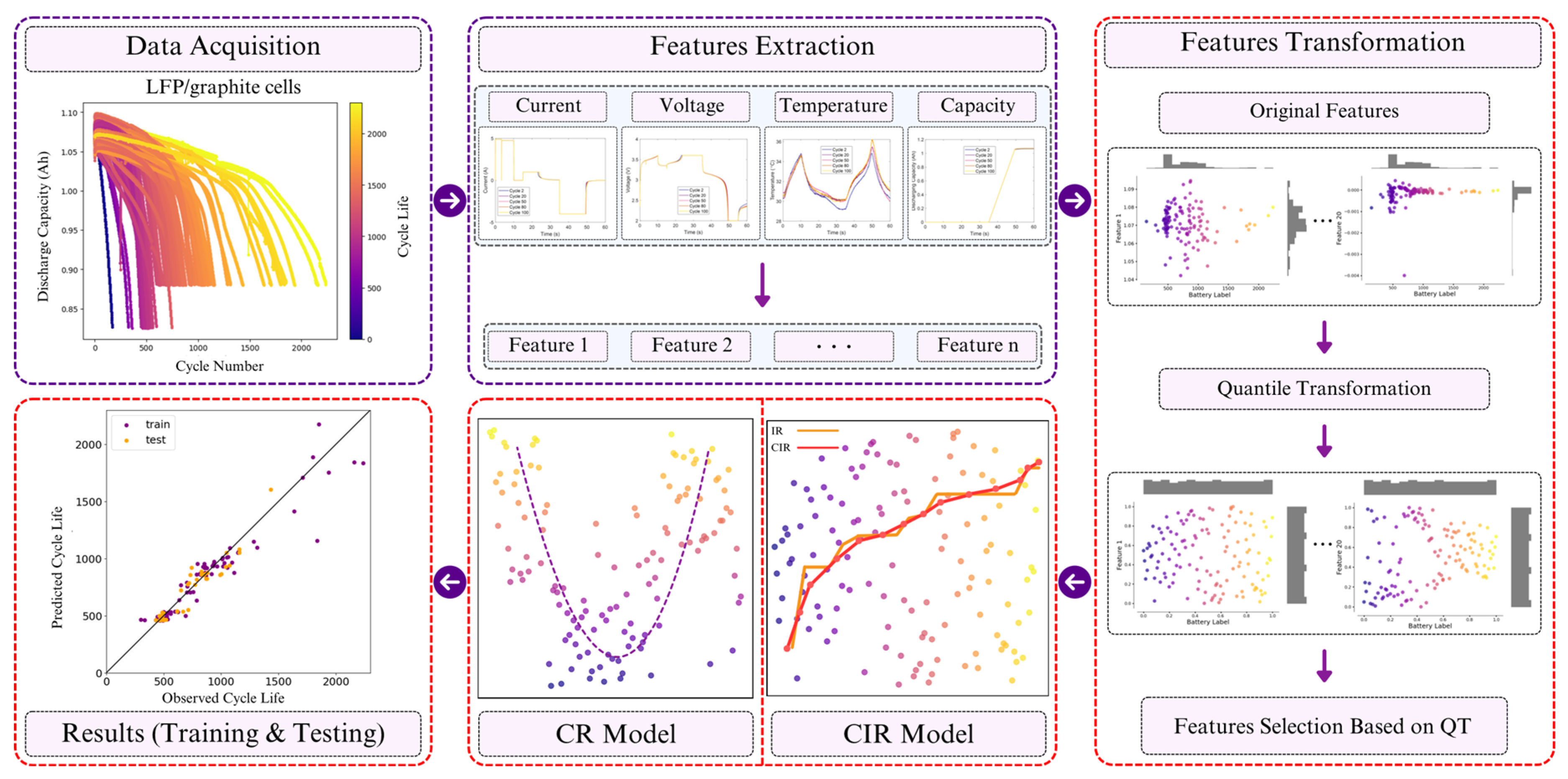
2.5. Data-Driven Framework for Battery Lifetime Prediction

The framework initiates with the collection of cycle data from LFP/graphite cells, where discharge capacity is recorded over multiple cycles, each reflecting varying stages of the cell’s lifecycle. After that, some features are extracted: current, voltage, temperature, and capacity, leading to a multi-dimensional feature space within which important information regarding the battery operation is captured, as shown in Figure 1. These features are transformed using QT, mitigating the influence of outliers with a uniform distribution, improving both stability and the performance of predictive models. After the QT transformation, the most significant features are selected for battery RUL prediction using proposed regression techniques.

The next step involves developing two predictive models: CIR and CR. The CIR model effectively captures the relationship between features and battery cycle lives by reducing overfitting, leading to more accurate and organized predictions. The CR is applied to fit a convex function to the data, effectively capturing specific patterns observed in the dataset where monotonicity is insufficient. The model performance is evaluated by comparing predicted and observed battery cycle lives. The proposed model demonstrates significantly better performance in predicting battery lifetime.

3. Dataset and Feature Analysis

3.1. Dataset Description

In this study, we employ the MIT battery dataset provided by Severson et al. [6], which contains 124 publicly available commercial LFP/graphite A123 APR18650M1A batteries with a 1.1 Ah nominal capacity and 3.3 V nominal voltage. These batteries experienced diverse fast charging conditions ranging from 3.6 C to 6 C with constant current-constant voltage (CC-CV). All batteries followed a uniform discharge protocol. Charging from a 0% to a 80% state of charge (SOC) used single or dual step policies with fixed C-rates over defined SOC intervals (e.g., 6 C from 0 to 50% SOC, then 4 C to 80%). Batteries then charged from 80% to 100% SOC through a 1C CC-CV protocol, terminating at 3.6 V (cutoff: C/50), and discharged at 4 C to 2.0 V (cutoff: C/50). The dataset comprises 124 cells, with each cell involving cycle life, charge policy, and structural summary, incorporating parameters such as cycle number, discharging capacity, charging capacity, IR, maximum temperature, average temperature, minimum temperature, and charging duration, along with cycle-related features. These batches are classified by considering the sequential order of the battery cell production under varying environmental conditions. Particularly, the dataset comprises scalar variables, including dynamic features such as voltage, current, capacity, temperature, and IR, all subject to continual changes over time. A cycle is deemed complete upon a full charging and later discharging. The lifecycle of all batteries spans from 148 to 2233 under 72 distinctive charging conditions in the controlled laboratory environment.

Analyzing the discharge capacity over the first 1000 cycles shows minimal capacity fade in the first 100 cycles, followed by an accelerated decline towards the end of battery life, a common trend in batteries. The intersection of the capacity fade curves emphasizes the weak correlation between the initial capacity and lifetime, an expected observation because of the less degradation during the early cycles. Generally, in the dataset under investigation, 81% of the cells exhibit an increase in capacity after 100 cycles, underscoring the significance of factors beyond mere capacity measurements. The small increases in capacity after a slow cycle or rest period could be caused by the charge stored in the area of the negative electrode, which is outside the positive electrode’s bounds.

Recognizing the limited predictive capacity of the correlations mentioned above relies on capacity fade curves, and we choose an alternative data-driven strategy that covers a complete set of cycling data. This strategy includes full voltage profiles of each cycle and other measures that include cell internal resistance and temperature. These changes in data trends allow for broader and deeper analysis, highlighting the importance of predictive models. The feature extraction from raw data will be done using the approach outlined by Severson et al. [6]. The process of feature extraction is crucial for enhancing the accuracy of cycle life predictions.

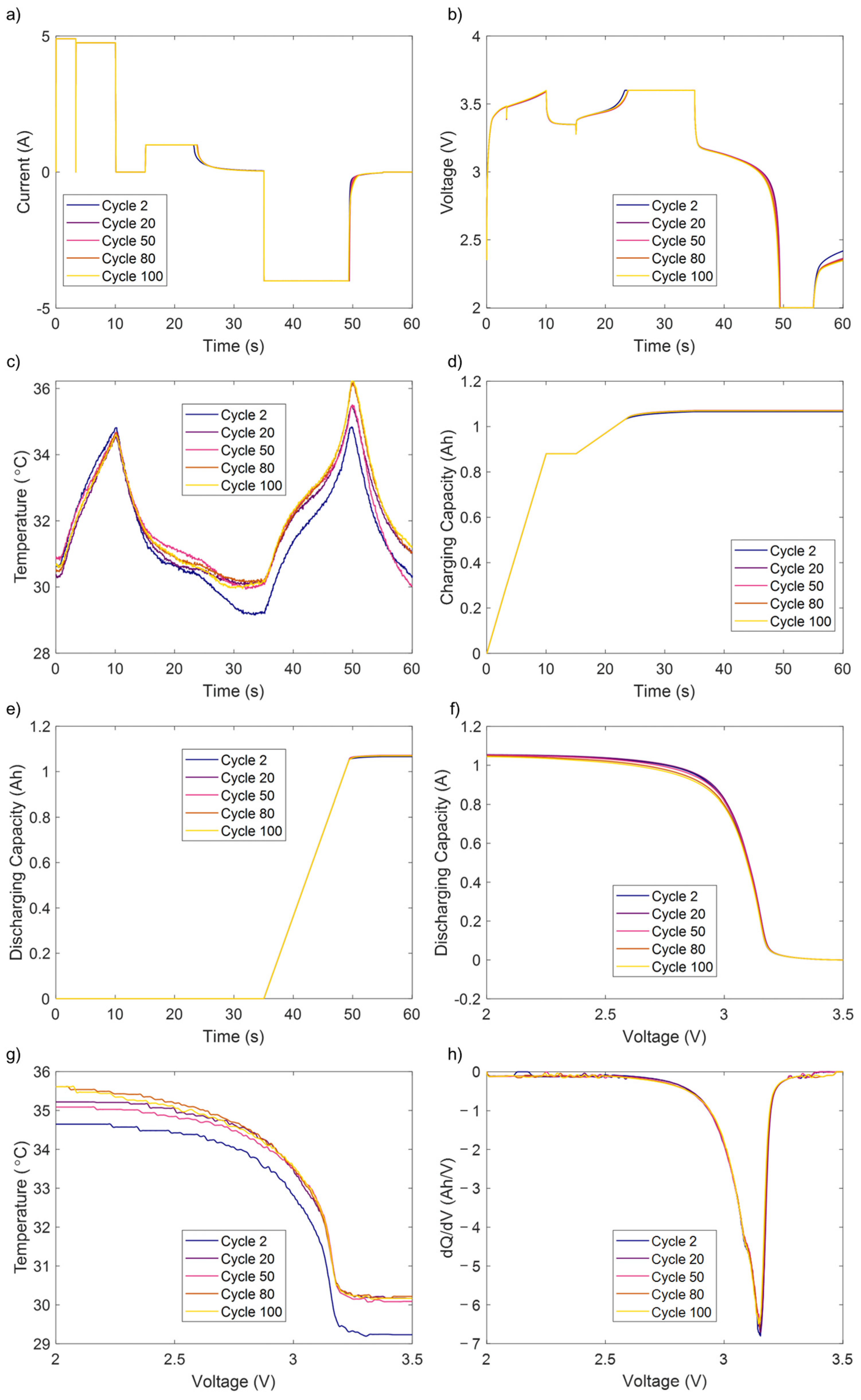
3.2. Features Extraction

Our work focuses on the first 100 cycles, taking into account the methodology proposed by Severson et al. [6]. In the complex aging dynamics of Li-ion batteries, several critical parameters effectively capture voltage, charge and discharge capacity, and temperature, as shown in Figure 2 [35].

The feature extraction is accomplished by obtaining 20 features, which are similar to the features in [6], to enable the models to accurately predict battery lifetime, while the details of the 20 features are listed in

Table A1. Features extraction from the MIT dataset for battery lifetime prediction [6].

Feature No.	Feature Details	Feature Representation
F-1	Discharge capacity at cycle 2	${QC}_2$
F-2	Difference between maximum discharge capacity and cycle 2	$\mathrm{M}\mathrm{a}\mathrm{x}({QC}_1,\dots ,{QC}_{100})-{QC}_2$
F-3	Discharge capacity at cycle 100	${QC}_{100}$
F-4	Integral of temperature over time, cycles 2–100	${\mathrm{I}\mathrm{n}\mathrm{t}T}_{2-100}$
F-5	Average charge time first 5 cycles	${\mathrm{A}\mathrm{v}\mathrm{g}t}_{1-5}$
F-6	Minimum of voltage discharge curve	$\mathrm{M}\mathrm{i}\mathrm{n}{Q}_{diff }\left(V\right)$
F-7	Mean of voltage discharge curve	$\mathrm{M}\mathrm{e}\mathrm{a}\mathrm{n}{Q}_{diff }\left(V\right)$
F-8	Variance of voltage discharge curve	$\mathrm{V}\mathrm{a}\mathrm{r}{Q}_{diff }\left(V\right)$
F-9	Skewness of voltage discharge curve	$\mathrm{S}\mathrm{k}\mathrm{e}\mathrm{w}{Q}_{diff }\left(V\right)$
F-10	Kurtosis of voltage discharge curve	$\mathrm{K}\mathrm{u}\mathrm{r}\mathrm{t}{Q}_{diff }\left(V\right)$
F-11	Value at 2V of voltage discharge curve	$Q_{diff }{|}_{V=2\mathrm{V}}$
F-12	Maximum temperature cycles 2–100	${\mathrm{M}\mathrm{a}\mathrm{x}T}_{2-100}\left(V\right)$
F-13	Minimum temperature cycles 2–100	${\mathrm{M}\mathrm{i}\mathrm{n}T}_{2-100}\left(V\right)$
F-14	Slope of the capacity fade curve, cycles 2–100	${\mathrm{S}\mathrm{l}\mathrm{o}\mathrm{p}\mathrm{e}CF}_{2-100}$
F-15	Intercept of the capacity fade curve, cycles 2–100	${\mathrm{I}\mathrm{n}\mathrm{t}\mathrm{p}CF}_{2-100}$
F-16	Slope of the capacity fade curve, cycles 91–100	${\mathrm{S}\mathrm{l}\mathrm{o}\mathrm{p}\mathrm{e}CF}_{91-100}$
F-17	Intercept of the capacity fade curve, cycles 91–100	${\mathrm{I}\mathrm{n}\mathrm{t}\mathrm{p}CF}_{91-100}$
F-18	Minimum internal resistance, cycles 2-100	${\mathrm{M}\mathrm{i}\mathrm{n}IR}_{2-100}$
F-19	Internal resistance cycle 2	${IR}_2$
F-20	Internal resistance difference between cycle 100 and cycle 2	${{IR}_{100}-IR}_2$

in the Appendix A. Initially, a range of different degradation data from the first 100 cycles is taken into consideration, where most cells do not reveal a significant capacity fade. The 20 features are analyzed in terms of sources and processes of extraction, hence giving a diversified overview with respect to battery aging dynamics. Specifically, geometric analyses and summary statistics of discharge voltage curves and derivatives provide the discharge capacity features, which are the most significant observations for battery degradation. This transformation $\Delta Q\left(V\right)$ conveys all the information in the discharge voltage curve and its derivatives, representing the most interesting point in effective degradation evaluation.

Additionally, features F-1 to F-20 are extracted from the discharge voltage curves, with F-1 representing the discharge capacity at cycle 2 and F-2 denoting the difference between the maximum discharge capacity and the capacity at cycle 2. F-3 corresponds to the discharge capacity at cycle 100, F-4 signifies the temperature integral over time from cycle 2-100, and F-5 manifests the average charge time across the first five cycles.

The next set of features, F-6 to F-11, are defined by summary statistics of the $Q_{diff }\left(V\right)$ curves, which characterize the difference in capacity between cycles 2–100; it is a critical feature in our analysis, including the minimum, mean, variance, skewness, and kurtosis, with F-11 comprising the value at 2 V for $Q_{diff }$. The features F-12 to F-17 emphasize capturing temperature variations and the behavior of the battery’s capacity degradation over time. F-12 and F-13 denote the maximum and minimum temperatures recorded from cycles 2 to 100, respectively. F-14 and F-15 describe the slope and intercept of the capacity fade curve from cycles 2 to 100, while F-16 and F-17 capture the slope and intercept of the capacity fade curve from cycles 91 to 100. For IR, F-18 is the minimum IR from cycle 2 to cycle 100, a measure of efficiency while in operation. F-19 actually gives the IR value of cycle 2; this is at the very start of cycling and provides a starting point from which all changes can be monitored. Finally, F-20 captures the difference in IR between cycle 100 and cycle 2, giving an idea of degradation and how that impacts the lifetime of the battery. Subsequently, the extracted features undergo feature selection, which aims to find the most critical indicators of battery degradation and performance.

4. Experimental Results

4.1. Feature Selection Using Quantile Transformation

In this section, the QT applied to the 20 features is a major preprocessing step that balances the varying distributions of the features, causing them to fall into a uniform distribution. It mitigates the effect of highly skewed distributions and outliers, making data consistent and easy to handle, which is mainly helpful for models sensitive to the distribution and size of the input data. The QT improves feature comparability and its correlations with the battery cycle life by distributing the data uniformly. The major result of this transformation is to equalize the distribution of each feature. This uniformity ensures that no single feature dominates the model due to scale or distribution, allowing for a more balanced input into the ML algorithms intended to deploy.

The features that most likely predict battery lifetime will be those that provide good, consistent trends with the battery’s cycle life. A feature that clearly exhibits a linear or non-linear trend and has a strong correlation with the battery cycle life may be an important predictor in the model. The modeling method should rank these features due to their high impact on the accuracy of the model.

Alternatively, features that exhibit a weak or unclear pattern with the battery cycle life may contribute less to the prediction. However, we cannot fully ignore such features, and their potential predictive power may require further transformation or feature engineering. One way to capture more complicated relationships that are not immediately evident in raw form is by generating polynomial features or interaction terms.

By considering each of the 20 features individually, we have noticed that features, such as F-1 to F-5, may show linear correlations with the battery cycle life. Even if these linear correlations are easy to model, redundancy should be avoided, especially if the features have a strong correlation with the battery cycle life. In such conditions, decreasing the number of features might enhance model performance by avoiding overfitting.

The F-6 offers a unique case because of its convex pattern. The non-linear connection implies a more complex relation between the feature and battery cycle life, maybe indicating a situation where performance increases to a certain extent before declining. It’s necessary to include this complexity in model as it is able to reflect a significant component of the underlying battery behavior that a simpler linear model might neglect. F-7 to F-10 exhibit a combination of linear and non-linear patterns, and their role in the model will depend on how strongly these features correlate with the battery cycle life. If these features show significant patterns, then they could be key predictors.

Similarly, F-11 to F-15 display varying degrees of correlation with the battery cycle life. The strongly correlated features are probably important indicators of battery lifetime, but weakly correlated features could need more adjustments to make them more helpful in the model. Lastly, F-16 to F-20 could display a range of patterns, from strong linear relationships to more complex, non-linear interactions, and understanding these relationships is vital for constructing a robust predictive model.

In addition to ordering these features, the QT method revealed the underlying linear and non-linear patterns of association between the features and the battery cycle life. The selection of modeling approaches and feature engineering methodologies is guided by these patterns, which guarantee that the model can accurately capture the complex patterns in the battery dataset. We used the correlation matrix generated with Pearson correlation, to guide feature selection after QT. We identified the 11 most highly correlated features with battery cycle life, while minimizing the inclusion of strongly inter-correlated features to avoid redundancy.

Based on the aforementioned discussion, we select the following 11 features: F-2, F-4, F-5, F-6, F-8, F-14, F-15, F-17, F-18, F-19, and F-20 for our regression CIR model. Currently, the features that strongly correlated or displayed significant patterns indicating predictive value with the battery cycle life are the ones that are shown in this selection. We propose a ML based method for the early prediction of Li-ion battery lifetime. This framework is composed of three main parts: feature transformation, feature selection, and ML based predictive modeling. Initially, a diverse set of 20 features is extracted from the raw degradation data to capture various aspects of battery aging dynamics. Subsequently, to address potential feature redundancy and irrelevance, the full feature set is transformed to produce a lower-dimensional subset, thereby enhancing the model’s predictive accuracy. This study uses the selected 11 features to evaluate the performance of various ML algorithms in terms of battery lifetime prediction.

This paper utilized 123 batteries from the MIT dataset, except for that with the shortest life, whose degradation pattern differed from other cells [24]. Stratified random sampling considers the intrinsic variability between the long-lived and short-lived cells in a given dataset for balanced representation. We divide the data so that 2/3 (83 samples) form the training set, and 1/3 (40 samples) constitute the testing set. This maintains the same ratio of long-lived to short-lived cells in the subsets [19]. We repeat the stratified random sampling procedure twenty times [20], to make the experiment less variable and average the results across these repetitions to make them reliable and robust.

This work uses two crucial statistical metrics, APE and RMSE, to compare the performance of our proposed method with other benchmarks. APE calculates the average percentage difference between the predicted and observed cycle lives, providing a valuable understanding of the overall accuracy of the predictive models. A lower APE value reflects a higher degree of accuracy and alignment between predicted and observed battery lifetimes, which means that the proposed method efficiently improves lifetime predictions. The APE is given as

$$\mathrm{A}\mathrm{P}\mathrm{E}\left(\%\right)={\displaystyle \frac{1}{N}}{\sum }_{i=1}^N{\displaystyle \frac{\left|y_i-{\widehat{y}}_i\right|}{y_i}}\times 100\%$$

(4)

where $y_{i }$ represents the observed cycle life, ${\widehat{y}}_i$ denotes the predicted cycle life, and the total number of battery samples is N. In contrast, RMSE provides a total measure of the magnitude of the differences between predicted and actual cycle lives, capturing variance and bias in the predictive models. The RMSE is stated as

$$\mathrm{R}\mathrm{M}\mathrm{S}\mathrm{E}=\sqrt{{\displaystyle \frac{1}{N}}\sum _{i=1}^N{\left(y_i-{\widehat{y}}_i\right)}^2}$$

(5)

RMSE figures out the differences between the predicted and observed cycle lives to show how well the prediction model works overall; lower RMSE values mean that the model is more accurate and reliable at predicting battery lifetimes.

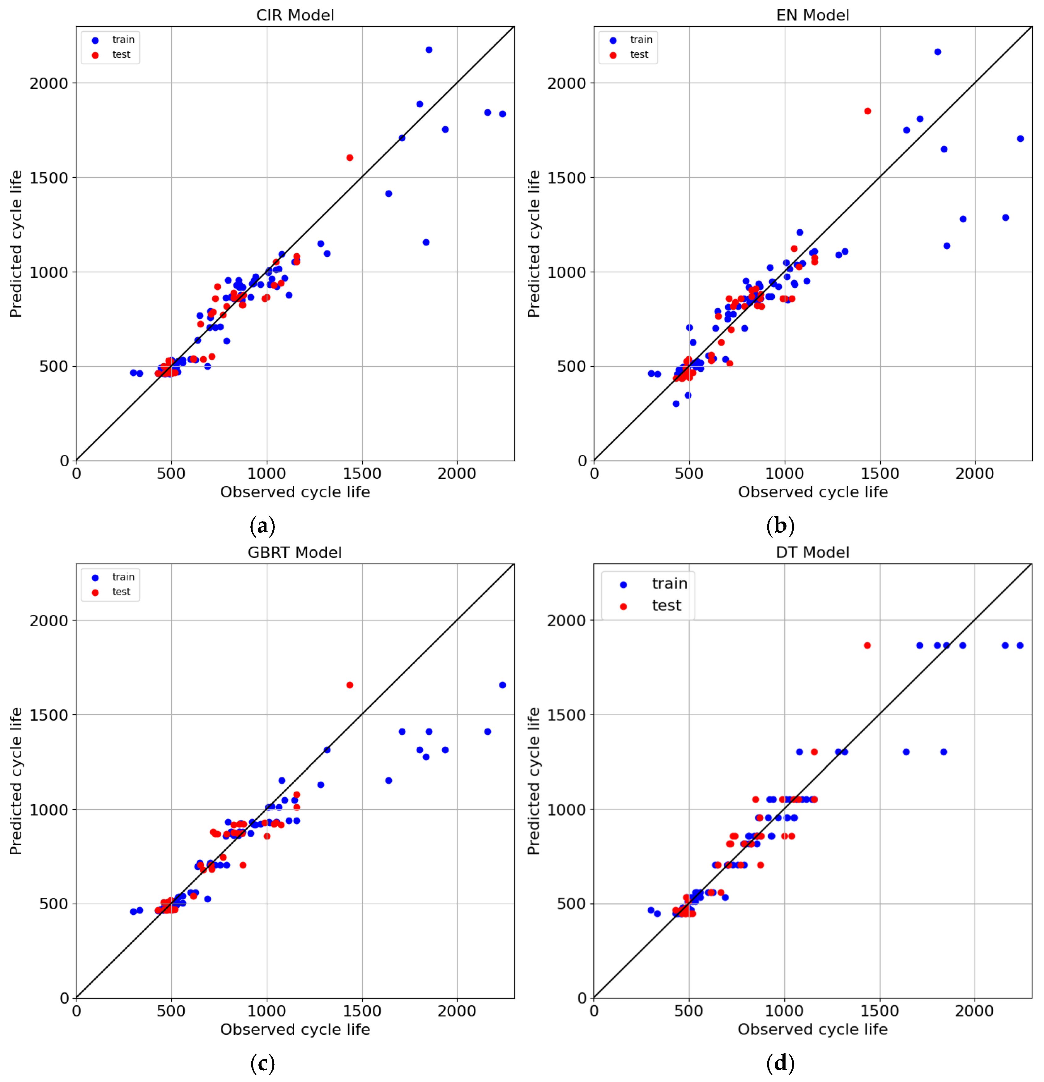
4.2. Results Comparison with Benchmarks

This section employs the CIR approach to predict battery cycle life and compares it with several ML techniques, including EN [6], GBRT [19], DT [19], SVM [19], RF [20], and GPR [20]. In the SVM model, we adopt the medium Gaussian kernel function. In the GPR model, we choose the exponential kernel function. As discussed in Section 4.1, we split the dataset into two parts: 2/3 for training and 1/3 for testing. To ensure its validity, we executed stratified random sampling and repeated for 20 times. Performance metrics give the average results over multiple iterations as an evaluation of predictive accuracy for each model.

The metric results are summarized in

Table 1. Model metrics for different prediction methods.

Model	APE (%)		RMSE (Cycles)
	Train	Test	Train	Test
CIR Model	7.3	9.8	120	149
EN	8.9	10.8	172	179
GBRT	7.7	10.8	161	181
DT	6.5	11.3	107	157
SVM	9.7	11.5	210	214
RF	8.5	11.4	206	217
GPR	8.6	10.4	164	180

, which compares the predictive performance of the CIR method with that obtained from other models. Utilizing a total of 11 selected features as input, CIR performed better than alternative methods for the two criteria of APE and RMSE. This advantage is because CIR accounts for monotonicity in the data, which usually occurs in battery lifetime predictions. Figure 3 shows the relationship between observed and predicted battery lifetime. The x-axis represents the observed values, the y-axis represents the predictions, and the blue and red dots indicate the training and testing results, respectively.

The evaluation provided APE values of 9.8% and RMSE of 149 cycles, respectively, for the CIR method. These findings highlight the accuracy of the CIR method compared to traditional models including, EN and SVM, which show higher error rates. The EN model showed an APE of 10.8%, with RMSE values of 179 cycles. While EN effectively balances the limitations of regression techniques, it struggles to capture complex patterns, which are reflected in its relatively high error rates, signifying less accurate predictions.

Similarly, GBRT achieved an APE of 10.8%, with RMSE values of 181 cycles. Despite its ability to manage non-linear patterns and reduce bias, GBRT is prone to overfitting, particularly with smaller datasets, as indicated by its elevated RMSE. The DT model obtained an APE of 11.3%, with RMSE values of 157 cycles. While DT is easy to interpret, they often overfit, as evidenced by the significant increase in RMSE, indicating weaker generalization.

The SVM demonstrated an APE of 11.5%, with RMSE values of 214 cycles. While SVM excels in handling high-dimensional data, these models can be computationally expensive and sensitive to kernel selection. The high RMSE values suggest challenges in fitting the model to the complex patterns present in the data. The RF model obtained an APE of 11.4%, with RMSE values of 217 cycles. However, RF is robust and effective at minimizing overfitting; it cannot directly account for patterns in the data.

Finally, the GPR achieved an APE of 10.4%, with RMSE value of 180 cycles. While GPR offers a probabilistic approach to regression, it faces scalability challenges and high computational costs, particularly with large datasets, leading to risks of overfitting, as suggested by its performance metrics.

5. Conclusions

This paper demonstrated the effectiveness of a data-driven methodology for early Li-ion battery lifetime prediction using QT, CIR, and CR. A key outcome of this work is the collaborative benefit of combining these methods to address challenges related to non-normality, outliers, and complex degradation patterns in battery data. QT enhances correlations between features and battery cycle lives, facilitating the discovery of stronger and more generalized relationships. CIR, a modified IR variant incorporating centering, mitigates overfitting while improving the model’s ability to capture hidden monotonic trends. Moreover, CR enables the accurate modeling of specific degradation patterns, further enhancing predictive accuracy.

The results highlight the significant potential of data-driven approaches for early-stage battery lifetime prediction. The achieved APE of 9.8% and RMSE of 149 cycles on the MIT dataset compare favorably with existing ML methods, demonstrating the practical applicability of the proposed methodology for battery optimization and management. A key insight from this study is the importance of accounting for the intrinsic characteristics of battery degradation data when selecting and integrating modeling techniques. While QT, CIR, and CR have been explored in various applications, their combination for early battery lifetime prediction yields notable performance improvements.

Future work includes extending this approach to other battery chemistries and datasets, exploring advanced feature engineering and selection techniques incorporating physics-informed features to enhance predictive accuracy. Additionally, optimizing computational efficiency will be crucial for scaling the method to real-world battery management systems.

References

1. Bhadriraju, B.; Kwon, J.S., II; Khan, F. An Adaptive Data-Driven Approach for Two-Timescale Dynamics Prediction and Remaining Useful Life Estimation of Li-Ion Batteries. Comput. Chem. Eng. 2023, 175, 108275. [Google Scholar] [CrossRef]
2. Cho, S.; Jeong, H.; Han, C.; Jin, S.; Lim, J.H.; Oh, J. State-of-Charge Estimation for Lithium-Ion Batteries under Various Operating Conditions Using an Equivalent Circuit Model. Comput. Chem. Eng. 2012, 41, 1–9. [Google Scholar] [CrossRef]
3. Cui, X.; Shen, W.; Zhang, Y.; Hu, C.; Zheng, J. Novel Active LiFePO4 Battery Balancing Method Based on Chargeable and Dischargeable Capacity. Comput. Chem. Eng. 2017, 97, 27–35. [Google Scholar] [CrossRef]
4. Homan, B.; ten Kortenaar, M.V.; Hurink, J.L.; Smit, G.J.M. A Realistic Model for Battery State of Charge Prediction in Energy Management Simulation Tools. Energy 2019, 171, 205–217. [Google Scholar] [CrossRef]
5. Wang, S.; Guo, D.; Han, X.; Lu, L.; Sun, K.; Li, W.; Sauer, D.U.; Ouyang, M. Impact of Battery Degradation Models on Energy Management of a Grid-Connected DC Microgrid. Energy 2020, 207, 118228. [Google Scholar] [CrossRef]
6. Severson, K.A.; Attia, P.M.; Jin, N.; Perkins, N.; Jiang, B.; Yang, Z.; Chen, M.H.; Aykol, M.; Herring, P.K.; Fraggedakis, D.; et al. Data-Driven Prediction of Battery Cycle Life before Capacity Degradation. Nat. Energy 2019, 4, 383–391. [Google Scholar] [CrossRef]
7. Wang, D.; Yang, F.; Tsui, K.L.; Zhou, Q.; Bae, S.J. Remaining Useful Life Prediction of Lithium-Ion Batteries Based on Spherical Cubature Particle Filter. IEEE Trans. Instrum. Meas. 2016, 65, 1282–1291. [Google Scholar] [CrossRef]
8. Zheng, X.; Fang, H. An Integrated Unscented Kalman Filter and Relevance Vector Regression Approach for Lithium-Ion Battery Remaining Useful Life and Short-Term Capacity Prediction. Reliab. Eng. Syst. Saf. 2015, 144, 74–82. [Google Scholar] [CrossRef]
9. Burgess, W.L. Valve Regulated Lead Acid Battery Float Service Life Estimation Using a Kalman Filter. J. Power Sources 2009, 191, 16–21. [Google Scholar] [CrossRef]
10. Micea, M.V.; Ungurean, L.; Cârstoiu, G.N.; Groza, V. Online State-of-Health Assessment for Battery Management Systems. IEEE Trans. Instrum. Meas. 2011, 60, 1997–2006. [Google Scholar] [CrossRef]
11. He, W.; Williard, N.; Osterman, M.; Pecht, M. Prognostics of Lithium-Ion Batteries Based on Dempster-Shafer Theory and the Bayesian Monte Carlo Method. J. Power Sources 2011, 196, 10314–10321. [Google Scholar] [CrossRef]
12. Yang, F.; Wang, D.; Xing, Y.; Tsui, K.L. Prognostics of Li(NiMnCo)O2-Based Lithium-Ion Batteries Using a Novel Battery Degradation Model. Microelectron. Reliab. 2017, 70, 70–78. [Google Scholar] [CrossRef]
13. Hu, C.; Ye, H.; Jain, G.; Schmidt, C. Remaining Useful Life Assessment of Lithium-Ion Batteries in Implantable Medical Devices. J. Power Sources 2018, 375, 118–130. [Google Scholar] [CrossRef]
14. Chen, X.; Liu, X.; Shen, X.; Zhang, Q. Applying Machine Learning to Rechargeable Batteries: From the Microscale to the Macroscale. Angew. Chemie 2021, 133, 24558–24570. [Google Scholar] [CrossRef]
15. Liu, D.; Zhou, J.; Liao, H.; Peng, Y.; Peng, X. A Health Indicator Extraction and Optimization Framework for Lithium-Ion Battery Degradation Modeling and Prognostics. IEEE Trans. Syst. Man Cybern. Syst. 2015, 45, 915–928. [Google Scholar] [CrossRef]
16. Nuhic, A.; Terzimehic, T.; Soczka-Guth, T.; Buchholz, M.; Dietmayer, K. Health Diagnosis and Remaining Useful Life Prognostics of Lithium-Ion Batteries Using Data-Driven Methods. J. Power Sources 2013, 239, 680–688. [Google Scholar] [CrossRef]
17. Zhang, Y.; Feng, X.; Zhao, M.; Xiong, R. In-Situ Battery Life Prognostics amid Mixed Operation Conditions Using Physics-Driven Machine Learning. J. Power Sources 2023, 577, 233246. [Google Scholar] [CrossRef]
18. Paulson, N.H.; Kubal, J.; Ward, L.; Saxena, S.; Lu, W.; Babinec, S.J. Feature Engineering for Machine Learning Enabled Early Prediction of Battery Lifetime. J. Power Sources 2022, 527, 231127. [Google Scholar] [CrossRef]
19. Yang, F.; Wang, D.; Xu, F.; Huang, Z.; Tsui, K.L. Lifespan Prediction of Lithium-Ion Batteries Based on Various Extracted Features and Gradient Boosting Regression Tree Model. J. Power Sources 2020, 476, 228654. [Google Scholar] [CrossRef]
20. Fei, Z.; Yang, F.; Tsui, K.L.; Li, L.; Zhang, Z. Early Prediction of Battery Lifetime via a Machine Learning Based Framework. Energy 2021, 225, 120205. [Google Scholar] [CrossRef]
21. Zhang, Y.; Peng, Z.; Guan, Y.; Wu, L. Prognostics of Battery Cycle Life in the Early-Cycle Stage Based on Hybrid Model. Energy 2021, 221, 119901. [Google Scholar] [CrossRef]
22. Fei, Z.; Zhang, Z.; Yang, F.; Tsui, K.L.; Li, L. Early-Stage Lifetime Prediction for Lithium-Ion Batteries: A Deep Learning Framework Jointly Considering Machine-Learned and Handcrafted Data Features. J. Energy Storage 2022, 52, 104936. [Google Scholar] [CrossRef]
23. Gong, D.; Gao, Y.; Kou, Y.; Wang, Y. Early Prediction of Cycle Life for Lithium-Ion Batteries Based on Evolutionary Computation and Machine Learning. J. Energy Storage 2022, 51, 104376. [Google Scholar] [CrossRef]
24. He, N.; Wang, Q.; Lu, Z.; Chai, Y.; Yang, F. Early Prediction of Battery Lifetime Based on Graphical Features and Convolutional Neural Networks. Appl. Energy 2024, 353, 122048. [Google Scholar] [CrossRef]
25. Zhao, W.; Ding, W.; Zhang, S.; Zhang, Z. Yong. A deep learning approach incorporating attention mechanism and transfer learning for lithium-ion battery lifespan prediction. J. Energy Storage 2024, 75, 109647. [Google Scholar] [CrossRef]
26. Zhang, Y.; Xiong, R.; He, H.; Pecht, M.G. Lithium-Ion Battery Remaining Useful Life Prediction With Box–Cox Transformation and Monte Carlo Simulation. IEEE Trans. Ind. Electron. 2019, 66, 1585–1597. [Google Scholar] [CrossRef]
27. Mahedy Hasan, S.M.; Uddin, M.P.; Al Mamun, M.; Sharif, M.I.; Ulhaq, A.; Krishnamoorthy, G. A Machine Learning Framework for Early-Stage Detection of Autism Spectrum Disorders. IEEE Access 2023, 11, 15038–15057. [Google Scholar] [CrossRef]
28. Pedregosa, F.; Varoquaux, G.; Gramfort, A.; Michel, V.; Thirion, B.; Grisel, O.; Blondel, M.; Müller, A.; Nothman, J.; Louppe, G.; et al. Scikit-Learn: Machine Learning in Python. J. Mach. Learn. Res. 2012, 12, 2825–2830. [Google Scholar]
29. Müller, M.; Huber, F.; Arnaud, M.; Kraemer, A.I.; Altimiras, E.R.; Michaux, J.; Taillandier-Coindard, M.; Chiffelle, J.; Murgues, B.; Gehret, T.; et al. Machine Learning Methods and Harmonized Datasets Improve Immunogenic Neoantigen Prediction. Immunity 2023, 56, 2650–2663.e6. [Google Scholar] [CrossRef]
30. Barlow, R.E. Statistical Inference Under Order Restrictions: The Theory and Application of Isotonic Regression; John Wiley & Sons Ltd.: Oxford, UK, 1972. [Google Scholar]
31. Robertson, T. Order Restricted Statistical Inference; John Wiley & Sons Ltd.: Oxford, UK, 1988. [Google Scholar]
32. Oron, A.P.; Flournoy, N. Centered Isotonic Regression: Point and Interval Estimation for Dose–Response Studies. Stat. Biopharm. Res. 2017, 9, 258–267. [Google Scholar] [CrossRef]
33. Boyd, S.; Vandenberghe, L. Convex Optimization; Cambridge University Press: Cambridge, UK, 2004. [Google Scholar]
34. Simonetto, A. Smooth Strongly Convex Regression. arXiv 2021. [Google Scholar] [CrossRef]
35. Wang, Y.; Jiang, B. Attention Mechanism-Based Neural Network for Prediction of Battery Cycle Life in the Presence of Missing Data. Batteries 2024, 10, 229. [Google Scholar] [CrossRef]
Figure 1. The flowchart of our proposed method for predicting battery cycle life.
Batteries 11 00145 g001
Figure 2. Data visualization of a random LFP/graphite cell: (a) current vs. time; (b) voltage vs. time; (c) temperature vs. time; (d) charging capacity vs. time; (e) discharging capacity vs. time; (f) discharging capacity vs. voltage; (g) temperature vs. voltage. (h) incremental capacity (IC) curves vs. voltage.
Batteries 11 00145 g002
Figure 3. Battery cycle life prediction results of (a) CIR; (b) EN; (c) GBRT; (d) DT; (e) SVM; (f) RF; and (g) GPR.
Batteries 11 00145 g003aBatteries 11 00145 g003b