Abstract
Lithium-ion battery (LIB) electrolytes are generally composed of a mixture of organic hydrocarbons and lithium salt (e.g., LiPF6). Experimental density data for basic and realistic multicomponent mixtures are scarce in the literature, and a predictive model for electrolyte solution density is not yet widely available. This work resolves to create a simple predictive method that can be used to estimate the density of these mixtures. A model that accounts for intermolecular forces in the electrolyte mixture was developed and fitted to density data available in the literature that was internally vetted for consistency. The model exhibited high accuracy for single-component electrolyte mixtures, with most predictions falling within 1% of measured values and all predictions falling within 5%. The model was further extended to more realistic, multi-solvent electrolyte mixtures that exhibited similar accuracy. In addition, a novel, accurate method for computing absolute molar and mass fractions of multi-solvent mixtures with specified volumetric concentrations (e.g., 1.2 M LiPF6 in 1:1:1% vol. ethylene carbonate-EC/diethyl carbonate-DEC/dimethyl carbonate-DMC) is also described. The two separate approaches were combined to yield a modeling framework capable of computing molar concentrations and densities of all LIB electrolyte solutions based on LiPF6 loaded in any combination of EC, EMC, DEC, DMC, and PC. Additional ionic salt data for NaPF6 and LiFSI were also evaluated to illustrate the adaptability of the model to different salts and electrolytes. Once again, the model was successful, with most density predictions falling within 1% error and all falling within 5%. This work ultimately provides a simple, adaptable modeling framework for accurate prediction of electrolyte mixture densities.
1. Introduction
Commercial lithium-ion batteries (LIB) electrolytes are primarily comprised of a mixture of organic solvents (e.g., ethylene carbonate (EC), ethyl methyl carbonate (EMC), diethyl carbonate (DEC), dimethyl carbonate (DMC), propylene carbonate (PC), and an assortment of esters, ethers, etc.) and a lithium salt (e.g., LiPF6), which act as a medium for lithium-ion transport. There is a large body of literature considering various properties of LIB electrolytes (e.g., electrolytic conductivity, ion mobility, thermal stability, etc.), but little attention has been paid to the density of these systems. However, electrolyte solution density is an important parameter for battery development and modeling efforts because it is utilized as an input parameter to more complex experimental analyses [1,2,3,4,5,6,7] and modeling efforts [2,3,5,7], or as an approach verification for molecular modeling efforts [8,9]. There are currently no open-source models in the literature capable of predicting the density of these mixtures, and such a model would improve the technical community’s capabilities for LIB modeling, characterization, and design.
Data for LiPF6-based electrolyte mixture densities relevant to LIB applications are sparse in the literature and limited to eleven papers [2,3,4,5,6,7,8,9,10,11,12], to the best of the authors’ knowledge. Furthermore, the density data presented in these papers are generally limited to single component electrolyte solutions and have been determined by differing methods (i.e., experimental vs. computational). All the available data have been compiled and are provided in the Supplementary Material along with relevant pure solvent densities from the NIST database [12] and electrolyte solution density measurements from commercial electrolyte suppliers (Sigma Aldrich (St. Louis, MO, USA) and Solvionic (Toulouse, France)). All density data compiled for single electrolyte/LiPF6 mixtures are shown in Figure 1 along with best-fit polynomial expressions. Figure 1 illustrates the lack of relevant data available for these mixtures, especially over the range of relevant salt concentrations.
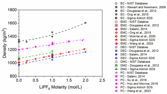
Figure 1.
Compilation of single-component electrolyte density data for LIB systems. Points correspond to data taken from the literature [2,3,4,5,6,7,8,9,10,11,12] and commercial electrolyte vendors (Solvionic and Sigma Aldrich), and lines correspond to polynomial fits.
Data provided by separate sources for similar conditions exhibits poor agreement in many cases. Some of the scatter observed in the data may be due to differences in temperature during experimental measurements, which are not always reported. Furthermore, the best-fit trend lines exhibit disparate shapes between electrolytes, but there is no fundamental reason for this behavior. The lack of numerous data points for some solvents (e.g., EC) and their high scatter illustrate the need for (1) accurate and widespread experimental measurements of electrolyte solution densities and/or (2) an accurate, predictive model to estimate the density for these solutions.
Hou and Monroe [2] previously correlated densitometry data for PC based on LiPF6 concentration with a polynomial expression which they argued was valid based on an analysis of Debye-Huckel theory [13] for ionic solutions. Similarly, Stewart and Newman [5] provided a linear correlation of experimental EC density measurements to LiPF6 concentration but did not provide justification for their mathematical expression. These correlations provide predictive capability for electrolyte densities but contain significant uncertainty and can only be utilized where experimental data are already available. The Advanced Electrolyte Model (AEM) [14] is a program developed by Idaho National Laboratory (INL) that can be purchased and is presently the most robust electrolyte model available. It can predict density for various electrolyte mixtures along with a wide variety of other properties that are relevant to electrochemical design. The density computation approach within AEMs framework is further discussed later in this paper.
Horsak and Slama [15] proposed a model to predict the densities of 1:1 aqueous electrolyte solutions based on each constituent chemical’s apparent molar volume. Their model included a parameter that accounts for the deviation of the system’s density based on interactions between the solvent molecules and the salt’s ions. Lam et al. [16] extended this model to predict the density of multicomponent ionic solutions with a wide variety of salts. The authors hypothesized that the modeling approach implemented by Horsak and Slama [15] and Lam et al. [16] could be extended to LIB electrolyte solutions and accurately predict their densities based on an intermolecular interaction parameter. Accordingly, Lam et al.’s [16] model is extended in the current study to electrolyte solutions typically used in LIBs and other novel battery electrolyte systems to accurately predict the solutions’ densities over a wide range of salt concentrations. The accuracy of the newly developed modeling approach is further demonstrated for prediction of solution densities for multicomponent electrolyte mixtures utilized in realistic LIB applications.
It should be noted that electrolyte density does not remain constant within a battery while under use. Concentration polarization (CP) can develop (more so at higher cycling rates), which causes electrolyte enrichment and higher density at one electrode. This phenomenon produces corresponding opposite effects at the counter electrode and creates a range of electrolyte property values across the battery. Regarding density, CP-driven electrolyte gradients will affect the local partial molar volume of solution.
In the following section, the modeling framework developed in the current study to estimate electrolyte solution densities is fully detailed. In addition, a method for computing the molar concentrations of all components in an electrolyte solution based on generally available data (i.e., provided by manufacturers and distributors) is developed. In the Results and Discussion section, the molar concentration estimation approach and density model are validated against data compiled from the literature and commercial vendors. The combined modeling approach is subsequently extended to realistic, multicomponent electrolyte mixtures and once again validated against the available data. Additional battery electrolyte mixtures are also evaluated to understand how well the model can be adapted to alternative or new salt/solvent systems. Finally, key findings and recommendations are provided in the Conclusion section.
2. Methods
2.1. Electrolyte Density Model
Common methods to predict densities of non-interacting systems include the rule of mixtures approaches (i.e., conservation of mass and volume approaches). Mixture density () computed with a conservation of mass approach is given by:
where and are the mass fraction and density of each component in the mixture, respectively. Similarly, mixture density computed with a conservation of volume approach is given by:
In both cases, Equations (1) and (2), the densities of LIB electrolyte mixtures are underpredicted, which indicates the presence of attractive intermolecular forces in these solutions. This finding is not unexpected because the presence of intermolecular forces in ionic solutions is a well-established result in the literature. Ion solvation is a well-known phenomenon that encompasses the dissociation of the individual salt ions within the solvent. The ionized molecules of the salt interact with the solvent molecules and reorganize the global molecular structure based on the strength and nature of each ion’s intermolecular interaction with the solvent. Literature on the solvation of the lithium ion within carbonate solvent molecules has investigated the development of the ion’s solvation shell [17,18]. The lithium ion is known to coordinate with the carbonate molecules via the carbonyl oxygen of the molecule and is understood to have a coordination number of 4 or 6. The small ionic size of the lithium ion coupled with a high-energy ion-dipole interaction leads to a local densification within the solvation regions and a corresponding reduction of the molar volume of the solution, as depicted in Figure 2, which accounts for the nonlinearity of these mixtures’ density trends (see Figure 1).
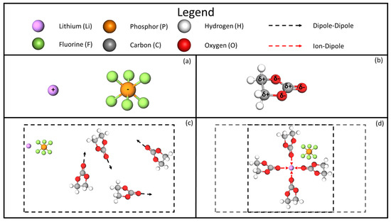
Figure 2.
Depiction of the molar volume densification phenomenon. (a) and ions. (b) A single EC molecule with overall dipole. (c) Four EC molecules with dipole-dipole interactions. (d) Four EC molecules attracted to the ion via ion-dipole interactions.
The modeling framework described by Lam et al. [16] is adapted in the current study to describe the solution density of LIB electrolytes. The electrolyte solution density is given by:
where and are the molar concentration and molecular weight of each component, respectively, and the subscripts , , and denote the salt, ionic molecules ( and ), and solvent, respectively. The solution’s molar volume () is given by:
where is the standard molar volume of each component and is the densification parameter, which is generally determined empirically. The densification parameter accounts for changes in the molar volume due to intermolecular forces between the salt ions and electrolyte molecules. This parameter explicitly quantifies the effects of the solvation process, which can involve several types of intermolecular interactions (i.e., hydrogen bonding, ion-dipole interactions, and van der Waals forces). Equations (3) and (4) can be further extended to electrolyte solutions containing multiple solvents:
where the subscript denotes the electrolyte solvent component (e.g., EC, DEC, etc.).
2.2. AEM Density Computation
AEM is a robust model capable of predicting a variety of electrolyte properties, including density, and is increasingly utilized as an industry standard for electrolyte modeling [14]. However, AEMs density prediction method has not previously been documented in the literature and has only been internally validated by INL employees. In this section, the AEM density modeling approach is outlined for comparison to the current study and experimental data later in the paper.
Density predictions within AEM utilize the molal basis to ensure a consistent methodology over a wide salt concentration range. This approach is used because the amount of total solvent present in the calculations will always be 1000 g, and this allows for differentiation between calculations via the solvent mass inputs. There are two primary cases for calculations that depend on the relative magnitude of solvent mass fraction of the first solvent (solvent 1, ) versus the remaining solvents (pseudo-cosolvent, ). The solvent mass proportions are assigned by the user. Pure component density values are supplied via the compound library in AEM, which corresponds to the void-free crystalline forms for salts.
The method used to compute mixture density () depends on the mass fraction of solvent 1 (). The first case is utilized when this mass fraction is greater than or equal to one-half (), which indicates the potential of a singular cosolvent. The specific volume of the solvent 1 and salt mixture is given by:
and the mixture density is the computed as:
where is the mass fraction of solvent 1 and the salt, is the mass fraction of the pseudo-cosolvent within the total mixture, and is the standard density of the cosolvent. The second case is utilized when the first solvent’s mass fraction is less than or equal to one-half (), which indicates the presence of higher mass concentrations of cosolvent(s). In this case, the specific volume of the cosolvent(s) and the salt is computed by:
where the density contribution of the cosolvent(s) are given by:
where is the mass fraction for the cosolvent for total cosolvents in the solvent mixture. The mixture density is finally computed as:
where is the mass fraction of all the cosolvents plus the salt in the mixture and is the mass fraction of solvent 1 in the mixture.
2.3. Baseline Properties
Standard densities, molecular weights, and molar volumes are required for each component and are provided in Table 1 for six organic solvents and a single salt that comprises most of the common LIB electrolytes. Densities presented for the pure solvents are taken from the NIST database [12] at STP conditions. Pure EC is a solid at STP conditions but melts at moderate temperatures (36 °C) and is a liquid in standard electrolyte mixtures, so the density value provided in Table 1 is an extrapolation of the liquid density from elevated temperatures. Molar volumes of the pure solvents were computed as the ratio of molecular weight divided by the standard liquid density ). Molar volumes for the salt ions ( and ) were calculated based on the ratio of their individual molar masses.

Table 1.
Baseline properties of electrolyte solvents, lithium salts, and ions.
2.4. Molar Concentration Computations
Molar concentrations of individual components are generally not provided in electrolyte solution data but are required by the current methods to compute solution densities. In general, LIB electrolyte solutions are specified in the following format: 1.2 M LiPF6 in 1:1:1%vol. EC/DEC/DMC, which is typically provided in a by-mass or volume format. The computational approach described in this section aims to compute molar concentrations of all solution components when the following information is known: (1) salt molarity (i.e., mol/L), (2) number and type of solvents, (3) relative mass or volume percentages of each solvent, and (4) solution density.
If relative solvent mass concentrations are provided, then the total mass of solvents () is calculated as:
where is solution density, is solution volume, is salt molarity, and is the salt’s molar mass. For simplicity, a solution volume of 1 L can be assumed in this approach, which implies the total number of salt moles is equal to its molarity ). The number of moles of each solvent () is then calculated as:
where and are the mass fraction and molar mass of the solvent, respectively. Molar concentrations of each component in the bulk solution are finally computed as the number of moles of each component divided by the total number of moles:
This method with provided relative solvent mass concentrations yields an exact solution for molar concentrations of each component.
In contrast, if relative solvent volume concentrations are provided by the manufacturer, then an exact method to compute molar fractions does not exist. A key assumption is made in the current analysis to circumvent this issue: the change in density resulting from the presence of salt ions is proportionally equivalent for every solvent. For example, if two solvents are mixed in a 1:1 ratio by volume before LiPF6 is added, then the solvents remain in a 1:1 ratio by volume afterwards. This assumption does not perfectly reflect the behavior of organic solvents, but it does provide accurate results for the solutions tested herein, as further discussed in the Results and Discussion section. If relative solvent volume concentrations are provided, then the total mass of solvents is calculated using Equation (12), but the number of moles of each solvent is computed by solving a system of linear equations:
where is the relative volume percentage of the th electrolyte solvent component, and any of the electrolyte solvent components can be arbitrarily selected for . The series of equations described by Equation (16) equates the volume of any of the solvents divided by its given volume percentage, which is simply the total volume of solvents. A solution volume of 1 L can again be assumed in this approach for simplicity, such that the total number of salt moles is equal to its molarity (). Finally, molar concentrations of each component are computed as before with Equation (14). Detailed example calculations for both cases (relative mass or volume concentrations provided) are provided in the Appendix A.
3. Results and Discussion
3.1. Molar Concentration Computations
The authors conducted a review of the relevant literature and documents provided by commercial vendors, which revealed that there is no published relative mass concentration data for any LIB electrolyte solutions that also includes specified relative solvent volume concentrations. However, these data are required to assess the accuracy and validate the volume-based approach to molar concentration computations developed here in Section 2.3. The authors reached out to commercial vendors and were able to obtain 8 sets of these data (5 from Solvionic and 3 from Sigma-Aldrich). The mass fractions (i.e., weight percentages) of all components were utilized to compute the exact molar fraction of all components. The component molar fractions were then approximated for the same 8 solutions with the volume-based approach previously described using the specified relative volume concentrations. The two computations are compared in the scatter plot of Figure 3, which illustrates the high accuracy of the volume-based approach and validates its underlying assumptions. The solid black line in Figure 3 represents perfect agreement. The average error of the computations was 1.4% with a maximum value of 9.6% and a coefficient of determination (R2) of 0.995. These results indicate that the volume-based approach can be used to compute molar fractions of solution components with high accuracy when relative mass fractions are not available.
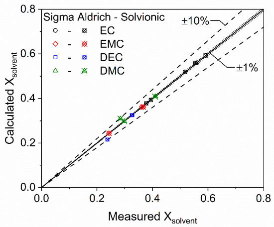
Figure 3.
Scatter plot of electrolyte solvent mole fractions as computed by the volume-based approach (calculated) compared to exact calculations (measured) completed with the mass-based approach.
3.2. Density Data Vetting Process
As previously noted (see Figure 1), density data for LIB electrolyte solutions were compiled from the literature and product specification documents provided by commercial vendors. These data were thoroughly vetted by the authors to remove any out-of-trend or potentially inaccurate data. A detailed description of the data vetting process and relevant rationale are provided in the Supplementary Material along with tabulations of the density data. In general, the sparse dataset suffers from a lack of reported significant figures, scatter between reported values at seemingly similar conditions, and general sparsity, which made determination of outliers difficult. The authors used their best judgment when vetting the available data, but the collection of further experimental data points in future research endeavors would improve the quality of this dataset and allow for refinement of the density model developed herein.
3.3. Single Component Electrolyte Mixtures
A nonlinear regression algorithm (fitnlm in MATLAB 2024a) was utilized to fit the single component density model (Equations (3) and (4)) to the vetted dataset and solve for relevant densification parameters (see Table 2). The nature of the model and single-salt data trends necessitated a single densification parameter to accurately describe the inherent intermolecular forces in these mixtures. Additional electrolyte data comprised of multiple salts in a single solvent could allow for the fitting of the parameter to individual ions and the production of ion-specific densification parameters.
Table 2.
Densification parameters for LiPF6 with electrolyte solvents.
A representative trend for solution density is shown in Figure 4 for PC. As previously discussed, the standard rule of mixtures approaches (Equations (1) and (2)) significantly underpredict the increase in solution density associated with LiPF6 addition. In contrast, the density model developed in the current study accurately captures this trend over a wide range of salt mass concentrations (≤0.25), which correspond to most battery-relevant salt molarities (0–2.1 M). AEM computations are also provided in Figure 4 for comparison, which also demonstrates good accuracy for the LiPF6-loaded PC mixtures without the inclusion of a direct densification parameter. However, such a parameter is intrinsic to AEM computations as evident in the term describing the difference in the inverses of the salt and solvent densities (see Equation (9)). This term is negative for the considered LIB salts and solvents in this paper and additionally scaled by the mass fraction of the salt.
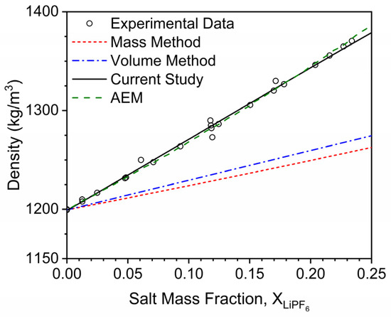
Figure 4.
The effect of LiPF6 addition on the density of PC. Points correspond to the data taken from the literature [2,3,4,5,6,7,8,9,10,11,12], and lines correspond to modeling approaches discussed herein. The solid black line represents the modeling approach developed in the current study, and the dashed orange line represents AEMs density predictions.
The capability and accuracy of the current density modeling approach are further demonstrated in the scatter plot of Figure 5 and the coefficients of determination presented for each single component electrolyte in Table 2. The majority of the data points lie within 1% error bands, and all lie within 5% error bands. The more significant outliers are for systems with sparser data, such as EC and DEC, where the authors are not as confident in the experimental data reported in the literature. However, the error associated with these predictions is still within an acceptable range, especially when the lack of another openly available modeling approach in the literature is considered. In general, good fits were achieved during the nonlinear regression analysis as evidenced by the high coefficients of determination for all single-component electrolyte mixtures (Table 2). Collection of more experimental density data for the systems with sparser data would further improve these fits and reduce potential prediction errors.
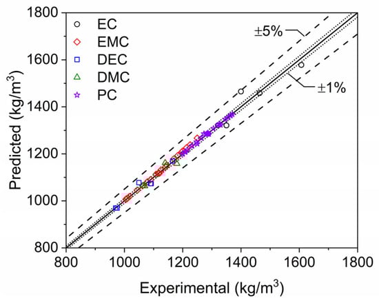
Figure 5.
Scatter plot of single-component electrolyte mixture densities. Densities computed at STP with the modeling approach developed in the current study (predicted) are compared to data reported in the literature [2,3,4,5,6,7,8,9,10,11,12] and by commercial electrolyte vendors (Solvionic and Sigma Aldrich).
3.4. Physical Originis of the Densification Parameter
The densification parameter represents the volumetric change of the solution as the salt ions interact with the solvent molecules. A deeper understanding of its physical origins was assessed by further probing fundamental parameters calculated from the AEM approach for single ions (cations and anions), ion pairs (IP), and triple ions (TI). First, the number of moles of salt per liter in each ion configuration that has been solvated with solvent molecules is calculated by:
where is the fraction of salt that exists as the ion species (cation, anion, IP, or TI) given by thermodynamic equilibrium, is the stoichiometric coefficient, and is the solvation number or the number of solvent molecules solvated with each ion species. The total molar population of solvators is found by the summation of Equation (17) for each cation, anion, IP, and TI result. The volume of solvent within the solvation shells for each ion species per liter of solution can then be calculated by:
where is Avogadro’s number, is the effective transport diameter based on the solvated state for each ion species, and is the unsolvated diameter for each ion species, which are both typically provided in Angstroms. The summation of each of these terms with respect to each ion species computes the total volume occupied by the solvators. With the total volume and molar population of the solvators, a computed AEM densification parameter can be calculated by:
where the computed densification parameter is in cm3/mol. This value can be calculated for each salt concentration point for each solvent in AEM, as shown in Figure 6. The AEM-computed densification parameter is not a constant value as assumed in the current study; it initially decreases in absolute value with increasing salt concentration and then increases with increasing salt concentration. An average computed densification parameter was obtained for each solvent over a LiPF6 concentration range of 0–2.0 M. The resultant values (Table 3) were close to the values defined in Table 2 in the current study for each respective solvent, excluding EC. The densification parameter computed for EC was −28.4 cm3/mol, which is far off from the value obtained from the model’s nonlinear regression (−86.963 cm3/mol). However, further investigation concluded that the model’s value is highly influenced by the two data points obtained from Stewart and Newman [7], while the single data point from Dougassa et al. [4] is more closely aligned with the computed densification parameter, as shown in Figure 7. Resulting in the conclusion that there is still merit with the defined meaning and calculations for a fundamental densification parameter. Additional density data would help to further this investigation to a concise conclusion.
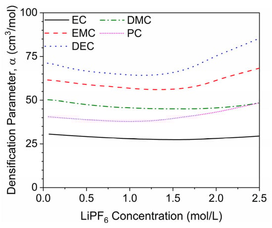
Figure 6.
Computed densification parameters from AEM modeling predictions for various electrolytes and over a range of LiPF6 concentration.
Table 3.
Comparison of densification parameters for LiPF6 with electrolyte solvents computed in the current study and with AEM.
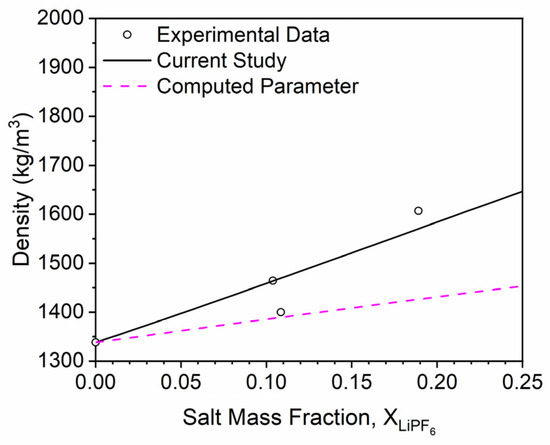
Figure 7.
The effect of LiPF6 addition on the density of EC. Points correspond to the data taken from the literature [2,3,4,5,6,7,8,9,10,11,12], and lines correspond to modeling approaches discussed herein. The solid black line represents the modeling approach developed in the current study, and the dashed magenta line corresponds to the same modeling approach utilizing an AEM-computed densification parameter.
3.5. Multicomponent Electrolyte Mixtures
The density model developed thus far provides accurate predictions of single-component electrolyte mixtures but is of little practicality unless it is capable of similar predictions for realistic, multicomponent electrolyte solvent mixtures utilized in LIB applications. The modeling framework was extended to multicomponent mixtures with Equations (5) and (6), and relevant densification parameters can be taken from the previously described regression analysis (Table 2). Density computations for multicomponent electrolyte solvent mixtures are compared to experimental data provided from the literature [2,3,4,5,6,7,8,9,10,11,12] and by commercial electrolyte vendors (Solvionic and Sigma Aldrich) in Figure 8. The majority of the data points lie within 2% error bands, and all lie within 5% error bands, except for a single outlier. However, the scatter of the predictions for multicomponent mixture computations is moderately worse than for the single component mixtures presented in the previous subsection. The source of this disparity is not clear but may be derived from uncertainty in the data reported by electrolyte vendors or the presence of solvent-to-solvent interactions in the solution that are not accounted for in the current modeling framework. Once again, the collection of more experimental density data for multicomponent electrolyte systems would further improve these fits and reduce potential prediction errors.
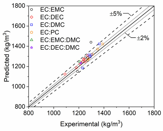
Figure 8.
Scatter plot of multicomponent electrolyte mixture densities. Densities computed at STP with the modeling approach developed in the current study (predicted) are compared to data reported in the literature [2,3,4,5,6,7,8,9,10,11,12] and by commercial electrolyte vendors (Solvionic and Sigma Aldrich).
3.6. Overall Accuracy of the Model
The evaluation of single and multicomponent mixtures individually illustrated the highly accurate predictive capability of the model presented in this paper. In its comparison to AEM, the authors wanted to evaluate both models for the entire range of LiPF6 data that was collected. A scatter plot comparing each of the model’s respective density predictions with their respective coefficients of determination is shown in Figure 9. AEM prediction values were taken at 25 °C and interpolated with respect to experimental mass fractions of the salt. Both models exhibit high accuracy in their predictions, with most predictions falling within 2% error and all, except for a few outliers, falling within 5% error. The outliers are from multi-component mixtures (EC:EMC) and for EC density data, where corresponding issues have been previously discussed. The model developed herein can thus predict electrolyte mixture density to a high degree of accuracy that is similar to AEM.
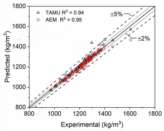
Figure 9.
Scatter plot of single- and multi-component electrolyte mixture densities. Densities computed at STP with the modeling approach developed in the current study (predicted) and the Advanced Electrolyte Model (AEM) [14] are compared to data reported in the literature [2,3,4,5,6,7,8,9,10,11,12] and by commercial electrolyte vendors (Solvionic and Sigma Aldrich).
3.7. Further Discussion
Separate approaches to compute molar concentrations of electrolyte solutions and predict the density of these solutions were developed. The former requires a known density as an input, and the latter requires known molar concentrations as an input. However, each approach has been independently validated in the current study. Accordingly, the separate approaches can be coupled and simultaneously solved in a fully predictive manner, such that their combination yields a modeling framework capable of computing molar concentrations and densities of any electrolyte solution based on LiPF6 loaded in any combination of EC, EMC, DEC, DMC, and PC regardless of the specification of their relative concentrations by mass or volume. This span of solutions encompasses the majority of all modern, commercial electrolyte solutions employed in LIB systems. Furthermore, the authors have developed a Python-based numerical algorithm that employs the models developed herein and solves them based on generally available electrolyte data (i.e., salt molarity and relative electrolyte solvent concentrations), which is available upon request. The modeling approach presented here and the accompanying code therefore negate the need for further experimental density measurements or similar modeling efforts by LIB researchers, potentially saving time and money in future battery development efforts. The exception to this statement is for the implementation of new electrolyte solvents or salts, but the authors suggest that the methods described here can be readily implemented in such cases to minimize experimental density measurements and associated efforts, as further discussed in the next section.
3.8. Additional Battery Salts
Additional data from the literature for other relevant battery salts and electrolytes was collected to illustrate the adaptability of the density prediction model developed here. In particular, density data for NaPF6 [19,20,21] and LiFSI [22,23] in single solvent and multicomponent solvent mixtures were collected. Physical properties of these salts were collected and utilized with the salt’s respective ion densification parameters to obtain coefficients for the new salt ions, as provided in Table 4 and Table 5, respectively. Similar quality fits were observed in comparison to the LiPF6 solutions as evidenced by the high coefficients of determination in Table 4. The coefficients of determination for both of the salts were calculated by determining how well the predictions from the model compared to all of the data (single and multicomponent mixtures).
Table 4.
Baseline properties of LiFSI and NaPF6 salts.
Table 5.
Densification parameters for additional salts with electrolyte solvents.
A representative density trend for LiFSI in PC is shown in Figure 10. Interestingly, the standard rule of the mixtures approach overpredicts the solution densities in this case. The values for the densification parameter are positive, which alludes to the decrease in density of these mixtures instead of densification. More investigation into the solvation of LiFSI would help elucidate the physical mechanism responsible for the observed behavior, but it is likely that the much higher density of the salt compared to the solvents negates the densification created by the ion’s solvation. AEM also overpredicts the density values, and the authors found that AEM was using a LiFSI density value (2500 kg/m3) higher than the one used in the current study (2320 kg/m3). Changing the density value within AEM produced a better fit but still overpredict values at increasing salt mass fraction.
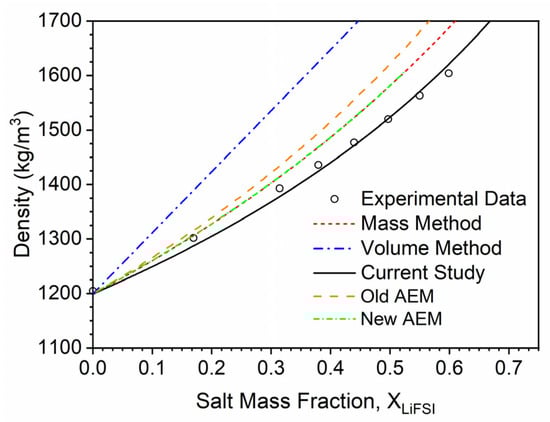
Figure 10.
The effect of LiFSI addition on the density of PC. Points correspond to the data taken from the literature [22], and lines correspond to modeling approaches discussed herein, with the green line being the trend from AEM with an updated salt density value. The solid black line represents the modeling approach developed in the current study.
The data for NaPF6 solutions primarily consisted of multi-solvent mixtures, which provided insufficient data to thoroughly investigate an increasing salt concentration trend for a single solvent mixture. Additional single solvent data for NaPF6 would allow for a similar analysis and further insight into the role of ion-dependent effects on mixture density. Nevertheless, the current study’s model is able to accurately adapt to the densification and density increase, as shown in Figure 11. This scatter plot illustrates the same predictive capabilities as observed with LiPF6, with most of the experimental data predicted within 1% error and all within 5% error for single and multi-solvent mixtures.
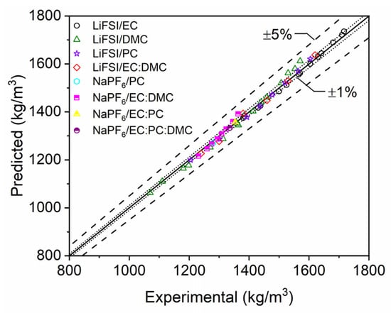
Figure 11.
Scatter plot of single- and multi-component electrolyte mixture densities with LiFSI and NaPF6. Densities computed with the modeling approach developed in the current study (predicted) are compared to data reported in the literature [19,20,21,22,23].
These additional computations illustrate the adaptive capabilities of the model developed here to accurately predict the densities of new battery salts and solvents. Additional analysis comparing the current study’s model to AEM is shown in Figure 12. AEMs density predictive capabilities were overpredictive for these additional salt mixtures, and predictions gradually worsened at increasing salt mass fractions. This is likely due to the lessened densification effect than what was seen with LiPF6 mixtures and the novel nature of the salts. However, the model outlined herein was able to adapt and produce accurate predictions over the studied range of salt mass fraction, with most predictions within 2% error and all within 5% error. Regarding AEM results in Figure 12, there are some cases of overprediction for LiFSI systems, which overall differ from the analogous results earlier with LiPF6 that showed little or no tendency toward overprediction. A simple reinvestigation of the pure-crystalline density of LiFSI could thus yield more precise density predictions for LiFSI electrolytes (as suggested by Figure 10).
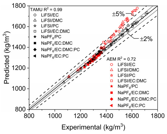
Figure 12.
Scatter plot of single- and multi-component electrolyte mixture densities with LiFSI and NaPF6. Densities computed at STP with the modeling approaches discussed herein (predicted) are compared to data reported in the literature [19,20,21,22,23].
4. Conclusions
LIB electrolyte density is a parameter that is important for battery development and modeling purposes because it is utilized for more complex experimental analyses [1,2,3,4,5,6,7] and modeling efforts [2,3,5,7], or as an approach verification for molecular modeling efforts [8,9]. However, the capability to accurately predict the density of simplified and realistic LIB electrolyte solutions does not currently exist in the open literature. The authors hypothesized that an existing solution density model [13,14] could be extended to LIB electrolyte solutions and accurately predict their densities based on an intermolecular interaction or densification parameter.
The current study was successful in developing and implementing separate models to compute individual component molar concentrations and solution densities for LIB electrolytes composed of organic solvents and lithium salts. The molar concentration calculation approach was validated against data collected from LIB electrolyte vendors and exhibited a high level of accuracy. The density model was validated for single-component electrolyte solutions against available literature data and data collected from vendors and subsequently validated for multicomponent electrolyte solutions. In both cases, the density modeling approach developed herein exhibited excellent accuracy. In addition, the current model was compared to AEM, which is the current industry standard and exhibited similar performance.
The two separate sub-models (i.e., molar concentration and density) have been combined, and the resultant computational model is capable of computing molar concentrations and densities of basic and realistic LIB electrolyte solutions in a fully predictive manner. The largest fault with the final modeling system presented herein is that it suffers from a lack of sufficient, high-quality experimental data for validation of its accuracy over a wide range of electrolyte formulations and conditions. The model is clearly capable of accounting for the effects of intermolecular forces on ionic solution densities, such as those encountered in standard LIB electrolytes, and can match all data in the existing literature within the limits of the data scatter and uncertainty. However, the accuracy and utility of this approach would significantly benefit from the collection of high-quality experimental density measurements for a range of basic and multicomponent LIB electrolyte solutions.
Furthermore, LIB electrolyte research is a highly active field with new solvents and salts constantly under investigation and development. Future work will be required to extend the current approach to any novel electrolyte formulations developed in the research and development sector. In the current study, the model was further extended to ionic salt mixtures based on NaPF6 and LiFSI, which illustrated its adaptability and continued high-level accuracy. It is the authors’ hope that this model will prove useful in the development of electrolytes for future batteries.
Supplementary Materials
The following supporting information can be downloaded at: https://www.mdpi.com/article/10.3390/batteries11020044/s1.
Author Contributions
Conceptualization, C.A.L. and J.C.T.; Data Curation, C.A.L., J.G.B. and J.C.T.; Formal Analysis, C.A.L., J.G.B., O.M., K.L.G. and J.C.T.; Methodology, C.A.L., J.G.B. and J.C.T.; Resources, J.C.T.; Software, K.L.G.; Validation, C.A.L., J.G.B. and J.C.T.; Visualization, C.A.L.; Writing—Original Draft, C.A.L., J.G.B. and J.C.T.; Writing—Review and Editing, O.M., K.L.G. and J.C.T.; Supervision, J.C.T.; Project Administration, J.C.T. All authors have read and agreed to the published version of the manuscript.
Funding
This research received no external funding.
Data Availability Statement
The data presented in this study are available in the Supplementary Material.
Acknowledgments
The authors would like to acknowledge scientists at Sigma Aldrich and Solvionic who were able to provide the mass breakdown of the multicomponent LIPF6 mixtures, which are not generally available to the public. This allowed for the validation of the molar concentration computation and proof that the method was accurate.
Conflicts of Interest
The authors declare no conflicts of interest.
Appendix A
Example molar concentration calculations demonstrating the mass-based and volume-based methods described in the current study are presented in this appendix. The mass-based example includes a 2 M LiPF6 solution with 2 solvents (4/6%wt. EC/EMC), and the volume-based example includes a 1 M LiPF6 solution with 3 solvents (1/1/1%vol. EC/DEC/DMC). Relevant baseline parameters for these calculations are provided in Table 1.
- Example 1: Mass-Based Method–Specified Relative Mass Concentrations:
Electrolyte Solvent Mixture: 2 M LiPF6 in 4/6%wt. EC/EMC
Density: 1270
Firstly, the total solvent mass is given by Equation (12):
where is the molar mass of the salt () and a total volume of 1 L is assumed for computational simplicity, which also implies . Next, the number of moles of each solvent, , is computed with Equation (13):
and, similarly, . Finally, each component’s molar fraction is calculated with Equation (14):
and, similarly, and .
- Example 2: Volume-Based Method–Specified Relative Volume Concentrations:
Electrolyte Solvent Mixture: 1 M LiPF6 in 1:1:1%vol. EC/DEC/DMC
Density: 1216
Firstly, the total solvent mass is given by Equation (12):
where is the molar mass of the salt (), and a total volume of 1 L is assumed for computational simplicity. Next, the system of equations provided by Equations (15) and (16) is simultaneously solved:
where the volume fractions of all components are equal in this case (). Simultaneous solving of these equations yields the moles of each component: , , and . Once again, a total volume of 1 L is assumed for computational simplicity, which also implies . Finally, each components’ molar fraction is calculated with Equation (14):
and, similarly, , , and .
References
- Lamb, J.; Orendorff, C.J.; Roth, E.P.; Langendorf, J. Studies on the Thermal Breakdown of Common Li-Ion Battery Electrolyte Components. J. Electrochem. Soc. 2015, 162, 12131–12135. [Google Scholar] [CrossRef]
- Hou, T.; Monroe, C.W. Composition-Dependent Thermodynamic and Mass-Transport Characterization of Lithium Hexafluorophosphate in Propylene Carbonate. Electrochim. Acta 2020, 332, 135085. [Google Scholar] [CrossRef]
- Wang, A.A.; Hou, T.; Karanjavala, M.; Monroe, C.W. Shifting-Reference Concentration Cells to Refine Composition-Dependent Transport Characterization of Binary Lithium-Ion Electrolytes. Electrochim. Acta 2020, 358, 136688. [Google Scholar] [CrossRef]
- Dougassa, Y.R.; Tessier, C.; Ouatani, L.E.; Anouti, M.; Jacquemin, J. Low Pressure Carbon Dioxide Solubility in Lithium-Ion Batteries Based Electrolytes as a Function of Temperature. Measurement and Prediction. J. Chem. Thermodyn. 2013, 61, 32–44. [Google Scholar] [CrossRef]
- Ong, T.M.; Verners, O.; Draeger, W.E.; van Duin, C.T.A.; Lordi, V.; Pask, E.J. Lithium Ion Solvation and Diffusion in Bulk Organic Electrolytes from First-Principles and Classical Reactive Molecular Dynamics. J. Phys. Chem. B 2015, 119, 1535–1545. [Google Scholar] [CrossRef]
- Su, L.; Darling, R.M.; Gallagher, K.G.; Xie, W.; Thelen, J.L.; Badel, A.F.; Barton, J.L.; Cheng, K.J.; Balsara, N.P.; Moore, J.S.; et al. An Investigation of the Ionic Conductivity and Species Crossover of Lithiated Nafion 117 in Nonaqueous Electrolytes. J. Electrochem. Soc. 2015, 163, A5253. [Google Scholar] [CrossRef]
- Stewart, S.; Newman, J. Measuring the Salt Activity Coefficient in Lithium-Battery Electrolytes. J. Electrochem. Soc. 2008, 155, A458. [Google Scholar] [CrossRef]
- Laoire, O.C.; Plichta, E.; Hendrickson, M.; Murkerjee, S.; Abraham, M.K. Electrochemical Studies of Ferrocene In a Lithium Ion Conducting Organic Carbonate Electrolyte. Electrochim. Acta 2009, 54, 656–6564. [Google Scholar] [CrossRef]
- Salami, N. Molecular Dynamics (MD) Study on the Electrochemical Properties of Electrolytes in Lithium-Ion Battery (LIB) Applications. Ph.D. Thesis, University of Wisconsin-Milwaukee, Milwaukee, WI, USA, 2014; p. 540. [Google Scholar]
- Lundgren, H.; Behm, M.; Lindbergh, G. Electrochemical Characterization and Temperature Dependency of Mass-Transport Properties of LiPF6 in EC:DEC. J. Electrochem. Soc. 2015, 162, A413. [Google Scholar] [CrossRef]
- Wang, A.A.; Persa, D.; Helin, S.; Smith, K.P.; Raymond, J.L.; Monroe, C.W. Compressibility of Lithium Hexafluorophosphate Solutions in Two Carbonate Solvents. J. Chem. Eng. Data 2023, 68, 805–812. [Google Scholar] [CrossRef] [PubMed]
- Linstrom, P.J.; Mallard, W.G. NIST Standard Reference Database Number 69. 2022. Available online: https://webbook.nist.gov/chemistry/ (accessed on 26 November 2024).
- Debye, P.; Hückel, R. The Theory of Electrolytes. I. Freezing Point Depression and Related Phenomena. Phys. Rev. 1923, 24, 185–206. [Google Scholar]
- Logan, E.R.; Tonita, E.M.; Gering, K.L.; Dahn, J.R. A Critical Evaluation of the Advanced Electrolyte Model. J. Electrochem. Soc. 2018, 165, A3350. [Google Scholar] [CrossRef]
- Horsak, I.; Slama, I. Densities of Aqueous Electrolyte Solutions. A Model for a Data Bank. J. Chem. Eng. Data 1986, 31, 434–437. [Google Scholar] [CrossRef]
- Lam, J.E.; Alvarez, N.M.; Galvez, E.M.; Alvarez, B.E. A Model for Calculating the Density of Aqueous Multicomponent Electrolyte Solutions. J. Chil. Chem. Soc. 2008, 53, 1393–1398. [Google Scholar] [CrossRef]
- Fulfer, K.D.; Kuroda, D.G. Solvation Structure and Dynamics of the Lithium Ion in Organic Carbonate-Based Electrolytes: A Time-Dependent Infrared Spectroscopy Study. J. Phys. Chem. C 2016, 120, 24011–24022. [Google Scholar] [CrossRef]
- Thomberg, T.; Väli, R.; Eskusson, J.; Romann, T.; Jänes, A. Potassium Salts Based Non-Aqueous Electrolytes for Electrical Double Layer Capacitors: A Comparison with LiPF6 and NaPF6 Based Electrolytes. J. Electrochem. Soc. 2018, 165, A3852. [Google Scholar] [CrossRef]
- Zhang, J.; Le, P. Electrolytes and Interfaces for Stable High-Energy Na-Ion Batteries; Pacific Northwest National Laboratory: Richland, WA, USA, 2021. [Google Scholar]
- Monti, D.; Jónsson, E.; Boschin, A.; Palacín, M.R.; Ponrouch, A.; Johansson, P. Towards standard electrolytes for sodium-ion batteries: Physical properties, ion solvation and ion-pairing in alkyl carbonate solvents. Phys. Chem. Chem. Phys. 2020, 22, 22768–22777. [Google Scholar] [CrossRef]
- Morales, D.; Chagas, L.G.; Paterno, D.; Greenbaum, S.; Passerini, S.; Suarez, S. Transport studies of NaPF6 carbonate solvents-based sodium ion electrolytes. Eletrochim. Acta 2021, 377, 138062. [Google Scholar] [CrossRef]
- Neuhaus, J.; Harbou, E.; Hasse, H. Physico-chemical properties of solutions of lithium bis(fluorosulfonyl)imide (LiFSI) in dimethyl carbonate, ethylene carbonate, and propylene carbonate. J. Power Sources 2018, 394, 148–159. [Google Scholar] [CrossRef]
- Wang, J.; Yamada, Y.; Sodeyama, K.; Chiang, C.H.; Tateyama, Y.; Yamada, A. Superconcentrated electrolytes for a high-voltage lithium-ion battery. Nat. Commun. 2016, 7, 12032. [Google Scholar] [CrossRef]
- European Chemicals Agency. Experimental Study: Lithium Bis(fluorosulfonyl)imide Density. 2013. Available online: https://chem.echa.europa.eu/100.212.319/ (accessed on 26 November 2024).
- Acros Organics, Material Safety Data Sheet: Sodium Hexafluorophosphate, 98.5+%. 2005. ACC#67823. Available online: https://pim-resources.coleparmer.com/sds/67823.pdf (accessed on 26 November 2024).
Disclaimer/Publisher’s Note: The statements, opinions and data contained in all publications are solely those of the individual author(s) and contributor(s) and not of MDPI and/or the editor(s). MDPI and/or the editor(s) disclaim responsibility for any injury to people or property resulting from any ideas, methods, instructions or products referred to in the content. |
© 2025 by the authors. Licensee MDPI, Basel, Switzerland. This article is an open access article distributed under the terms and conditions of the Creative Commons Attribution (CC BY) license (https://creativecommons.org/licenses/by/4.0/).