Abstract
Lithium-ion batteries with high active material loading can yield a high energy density at low C-rates. However, the sluggish ion transport caused by longer and more tortuous pathways hinders high energy delivery when extracting high power. This study presents the implementation of neural networks to optimize the gradient active material distribution profile throughout the thickness of electrodes to enhance energy density. The profiles were randomly generated, while maintaining a constant average active material in each electrode. An electrochemical–thermal model was used to investigate the impact of different profiles. A neural network model was then developed to establish the connection between the profiles and the resulting energy density for various electrode thicknesses and C-rates, utilizing a limited amount of simulation data. The neural network model could replicate the performance of the electrochemical–thermal model, but with significantly reduced computational time. This enabled the possibility of efficiently exploring a vast number of candidate profiles to identify the most optimal one for each of the positive and negative electrodes. The results showed that the gradient profiles were mostly influenced by the average active material, rather than the thickness of the electrode. Finally, at high currents, the optimal gradient profiles increased the energy density by over four times compared to uniform electrodes.
1. Introduction
Lithium-ion batteries (LIB) are promising energy storage systems that are widely used as the prime storage solution for electric vehicles and consumer electronics. These batteries have a high volumetric and gravimetric energy density compared to other types of rechargeable batteries, which makes them an ideal choice for mobile applications (e.g., electric vehicles), where the size and weight of the energy storage system are determining factors [1]. However, there is an increasing demand in industry for high energy–high power LIBs for electric vehicles, to achieve a comparable performance to that of internal combustion engines in terms of both mileage and acceleration [2].
LIB’s energy and power characteristics are greatly influenced by the geometric properties of the electrodes, specifically their thickness and porosity [3]. One simple method for enhancing the energy level of LIBs is to use thick electrodes with low porosity. The increased active material loading reduces the total weight and cost of the battery at the pack level, due to the reduced amount of non-active material used (e.g., current collectors) [4]. Despite this, the inherent limitation of this method is that these types of batteries are unable to maintain a high energy value at high C-rates, due to poor utilization of active material [5].
Electrochemical models such as the Doyle–Fuller–Newman (DFN) pseudo-two dimensional (P2D) model have been employed to study the effect of geometrical parameters and material properties on battery performance [6]. This model offers insights into charge and mass conservation mechanisms and reaction kinetics in both electrolyte and active electrode phases [7]. The resulting information provides an in-depth understanding of the effect of different parameters on battery dynamics during operation, facilitating rational guidance for LIB design prior to the manufacturing stage [8].
While analyzing the effect of each individual parameter using electrochemical models is possible, understanding the superimposed effect of multiple parameters on a desired characteristic might be challenging. In such a situation, one solution is to exhaustively search all the possible parameter combinations and select the set that fulfills the desired objective (e.g., high power and energy); however, such approaches are computationally intensive for high-dimensional parameter spaces. A more computationally efficient method is using an optimization method in combination with a physics-based model. Several studies have performed such a task. Liu et al. [9] performed an optimization task using a genetic algorithm to enhance the discharge capacity, specific energy, and power by considering electrode thickness, porosity, particle radius, and positive electrode conductivity as design variables. In another study, Xue et al. [10] used a gradient-based algorithm to identify the set of parameters that led to the highest possible energy density values for a minimum required power density at each operating C-rate by searching through a design space consisting of geometrical parameters and material properties. De et al. [11] conducted a simultaneous optimization task by finding the best combination of positive and negative electrode thicknesses and porosities. The goal was to enhance the energy level, without sacrificing the deliverable capacity compared to the base set of parameters.
Since there is a limit on the highest energy that can be achieved, even with an optimized thickness and porosity combination, batteries with gradient porosity electrodes have been suggested [12]. In such batteries, the porosity varies throughout the electrode thickness, rather than being constant. These electrodes have been constructed and experimentally tested to investigate their effectiveness. Yang et al. [13] fabricated a 3-layered graphite electrode by repeatedly coating and calendaring graphite slurries, resulting in a reduced capacity loss after 150 cycles in comparison to a single-layered electrode. Liu et al. [14] tested a double-layered cathode in combination with both Li metal and graphite. In comparison with a one-layered electrode, the double-layered cathode exhibited a lower capacity loss after 50 cycles. In addition to the conventional LIB electrodes, gradient structures have also been proven to be effective in other battery chemistries. Cao et al. [15] examined the effect of gradient pore volume, alongside gradient sodiophilic sites and electrical conductivity, resulting in enhanced cycling stability and improved energy density.
Some studies have focused on the analysis and optimization of the gradient profile of active material using electrochemical models. Ramadesigan et al. [16] studied the effect of the gradient porosity profile across the positive electrode thickness on the internal resistance. A simplified P2D model was employed, by ignoring the solid phase intercalation mechanism, with control vector parameterization (CVP) used as the optimization method. They obtained a 15–33% reduction in the internal resistance with a multi-layered electrode structure. Golmon et al. [17] investigated the effect of gradient porosity electrodes and particle radius on LIB performance using an electrochemical model. Their findings demonstrated that a gradient profile and small particle size improved the battery performance in terms of the maximum usable capacity and mechanical forces. Hosseinzadeh et al. [18] studied the effect of gradient porosity on heat generation, as well as the energy and power of the LIB. They introduced a multi-layered structure in both electrode thickness and height directions, leading to an 8.37% and 2.6% improvement for energy and power for an NMC–graphite cell, respectively, and a 4.2–14% reduction in cathode heat generation rate for an LFP cell. Zhou et al. [19] modified a two-dimensional model to assess the impact of electrode structure on the lithiation process, using varying sizes of active material particles to create a gradient within the electrode. Their results showed that the gradient structure improved the particle utilization near the current collector and reduced non-uniformity in solid-phase Li concentration across the electrode thickness, leading to enhanced electrochemical performance. Du et al. [20] investigated the effect of the gradient porosity profile on the energy level of thick cathodes by defining the porosity profiles as first- and second-degree polynomial equations. They reported a negligible improvement in energy at a 1.5C discharge rate with the profiles that had the lowest amount of active material next to the separator, while profiles with the opposite direction led to a decreased level of energy. Yu et al. [21] employed a pseudo-three-dimensional (P3D) electrochemical–thermal–mechanical (ETM) coupled model to investigate porosity gradients in the positive electrode. They analyzed the impact of porosity variation on battery temperature and stress during discharge, finding that the optimal porosity distribution promoted uniform electrode lithiation and lowered the surface temperature by reducing ionic ohmic heating.
Directly applying optimization methods to numerical models can be computationally demanding and often requires model simplification. Machine learning (ML) models provide a solution to this problem by capturing the intricate relationships between the inputs and outputs and directly linking design parameters to specific cell characteristics, without solving the underlying model equations. ML models offer fast computation capabilities, making them a viable choice for real-time LIB state estimation and offline design tasks. Developing a surrogate ML model for design applications involves defining a design space and training the model with a limited dataset derived from the simulations. Once properly trained, the ML surrogate model can replace the physics-based model and be employed, either in combination with an optimization algorithm, or to quickly predict the effect of large combinations of parameters.
Considering the potential of ML surrogate modeling, several studies have already leveraged this approach [22]. Wu et al. [23] used artificial neural networks (ANNs) for both classification and regression tasks to optimize the energy and power of LIBs. A classifier neural network was utilized to identify and eliminate the sets of parameters that led to electrolyte depletion from the design space. A regressor neural network was employed to calculate the energy and power values for each design set. Using this method, the computational cost was extensively reduced, facilitating a sensitivity analysis and design optimization. A similar study was conducted by Quartulli et al. [24], investigating the advantages of using ensemble classification methods such as voting, gradient stacking, and deep stacking ensemble over traditional ANNs. The method of data-driven surrogate modeling has also been used to study electrode structure. Gao et al. [25] studied a gradient electrode porosity profile by introducing a tapered shape electrolyte channel structure to reduce tortuosity and improve the specific energy, power, and capacity. A multi-input–multi-output neural network was used to map the channel structure parameters to the three selected performance metrics. A Markov chain Monte Carlo (MCMC) gradient descent optimization algorithm was then used alongside the data-driven model to perform the design optimization task. This resulted in a 79% improvement in energy density compared to the high-tortuosity electrode of the base case. In another study by Sui et al. [26], the effect of vasculature structure on the charge capacity was investigated using a simplified one-dimensional electrochemical model. The electrode structure was optimized under defined design scenarios using a bagging ensemble neural network, with mapping of the vasculature structure parameters and operating C-rate to the charge capacity. Miyamoto et al. [27] developed a framework for energy improvement of 3D micro batteries, using a transmission line model (TLM) and principal component regression model. They tested a huge number of randomly generated electrode geometries, and the energy value of each geometry was calculated using a machine learning model. Those geometries that resulted in improved energy values at both low and high C-rates were selected as the optimal ones.
Table 1 presents a summary of the most relevant studies on the effect of electrode structure on the specific energy of LIBs. As can be seen, the studies without optimization did not report a significant improvement. Those studies that optimized a gradient electrolyte channel structure using a ML surrogate model (references [25,26]) reported higher improvements. Miyamoto et al. [27] reported a significant improvement in specific energy by optimizing a randomly generated interdigitated electrode structure. However, the electrodes are considered to be very thick (around 600 m), which in combination with the interdigitated structure would make these types of electrodes quite difficult to manufacture, especially at large scale. Despite their findings, these studies were limited by not assessing the effect of different active material distributions for a range of thicknesses and average active material ratios.

Table 1.
A comparison of the previously conducted research on gradient electrodes with the current study.
In this study, a ML surrogate model was developed to find the optimal distribution of active material for both negative and positive electrodes. An electrochemical–thermal model was used to generate a training and test dataset by performing a parametric sweep over electrode thickness, average active material ratios, active material distribution profiles along the electrodes’ thickness, and different C-rates. The effect of active material distributions for a range of electrode thicknesses across four case studies was assessed. The introduced gradient active material distribution improved the energy levels at high C-rates, but the average ratio was also kept constant, which prevented sacrificing energy values at lower C-rates. The proposed active material functions have a piecewise cubic shape, comprising a combination of gradient and layered structures. Such structures are easier to manufacture and can be achieved using either layered structures alone or through a combination of in-plane channels and layered structures [28,29]. The low computational time requirements of the developed ML model provided the opportunity to study a large design space by performing an exhaustive search, without using an optimization algorithm.
2. Materials and Methods
This study investigated the effect of electrodes with gradient active material profiles on the energy density of an NMC–Graphite LIB, using a physics-based and data-driven model. Initially, gradient profiles were generated randomly under certain physically feasible constraints. Using an electrochemical–thermal model developed in COMSOL Multiphysics 6.1, the effect of the profiles on battery performance was investigated. A large dataset of simulation data was generated by varying the electrode thickness, the average active material ratio of each electrode, and the operating C-rate. The dataset was used to train the data-driven model, which aimed to identify the correlation between the selected design parameters and the energy density. The gradient profiles were described with 10 points that were evenly distributed along the thickness of the electrodes. Subsequently, the data-driven model was employed to efficiently compute the impact of numerous candidate profiles within a short time frame, resulting in the acquisition of frontier solutions that met the optimization criteria.
2.1. Electrochemical–Thermal Model
The P2D model is an electrochemical model for LIB simulation which assumes the electrodes are porous media consisting of spherical particles of active material, with a binary electrolyte filling the empty spaces among the pores [30]. The model describes the electrode-level behavior of the cell in the spatial direction of cell thickness (x-direction) and the particle-level behavior in the pseudo-direction of particle radius (r-direction) [31]. The governing equations of the model are represented in Table 2.

Table 2.
Summary of the governing equations of the P2D model.
The main variables described by the model include the solid and electrolyte phase potentials (V), and , and the Li+ ion concentrations in the solid particles and electrolyte (molm−3), and .
The parameters defining material properties at the electrode level must be corrected based on the active material ratio () or electrolyte ratio () at each point along the x-direction and using the Bruggeman constant (p):
where is the effective conductivity of the solid active material (S m−1), is the electrolyte diffusion coefficient (m2s−1), and is the effective electrolyte phase conductivity (S m−1). The active material ratio used for correcting the material properties changes along the electrode thickness:
where , and are the thicknesses of the positive electrode, negative electrode, and the separator, respectively. is the solid phase diffusion coefficient, which is not corrected, because it is only applicable at the particle level and there is no mixture of active material and electrolyte inside the particles, and (S m−1) is the effective diffusional conductivity defined as .
Other parameters of the governing equations include , which is the ratio of active surface area to the electrode volume, described as ; Faraday’s constant, F (C/mol); and the transference number, . The current density, i, is described by the Butler–Volmer kinetics equation, where is the overpotential (V), and are the anodic and cathodic charge transfer coefficients, R is the universal gas constant (J/molK), T is the temperature (K), and is the equilibrium potential for each electrode, as shown in Figure A1. is the exchange current density, which is a function of the Li+ ion concentration on the surface of the particles, (mol/m3), and the maximum Li+ ion concentration in solid phase, (mol/m3).
Heat is generated during the cell’s charging and discharging, and the internal temperature changes. The electrolyte properties are dependent on the cell temperature; therefore, it is important to consider the effect of temperature variation on the electrolyte properties. The parameters of the thermal model include the density, (kg/m3), the specific heat capacity, (J/kg K), the thermal conductivity, K (W/mK), and convective heat transfer coefficient, h (W/m2K). q is the total heat generation of the cell (Wm3), and consists of reaction, reversible, and ohmic heat generation terms.
In this work, positive electrode thickness and average active material ratio were considered as design variables with a defined range. Therefore, the cell capacity was calculated using positive electrode parameters based on the equation below:
where is the average solid active material ratio of the positive electrode, and and are the initial and final state of lithiation of the positive electrode during the discharge process.
The negative electrode was then calculated based on cell capacity and average negative electrode active material, which was another design variable.
When changing the negative electrode average active material ratio, the thickness was adjusted accordingly. In this way, we investigated the effect of different active material ratios, while balancing the areal capacity of each electrode, making sure that both positive and negative electrodes were used efficiently.
The applied current, (Am−2), was calculated as below:
Specific energy (Whkg−1) and power (Wkg−1) values were calculated from the equation below:
where is the cell voltage, and is the cell weight (kgm−2):
where the subscripts , , , e, and stand for current collectors, aluminum, copper, electrolyte, and binder and additives, respectively, and is the average electrolyte ratio of each electrode. Since the cell weight does not affect the partial differential equations, the effect of gradient porosity was not considered here and the average porosity values were used in the calculations.
Parameters used in the electrochemical–thermal model are shown in Table A1, Table A2, Table A3 in Appendix A. The units for the electrolyte concentration () and temperature (T) in the electrolyte property equations are based on mol/cm3 and K, respectively.
The developed model was used to analyze the effect of applying gradient active material profiles on the cell’s specific energy. These profiles were generated under the following assumptions: the ratio of binder and additive was considered to be 0.1, the minimum amount of solid active material in each electrode could not be below 0.2 (maximum electrolyte fraction is 0.7), and the maximum amount of solid active material was 0.8 (minimum electrolyte fraction is 0.1). Each profile consisted of 10 points that were evenly spaced along the electrodes’ thicknesses. The generated points were connected using the cubic-piecewise interpolation method, and the average active material ratio was equal to the area beneath the plot, which was numerically calculated with a tolerance of 0.001.
The points were generated under the condition that each point had to be smaller or equal to the point in front of it, so that the lowest amount of active material was next to the separator (higher porosity) and the highest amount was next to the current collectors (lower porosity), as depicted in Figure 1. The reason for such an assumption is shown in Figure 2.
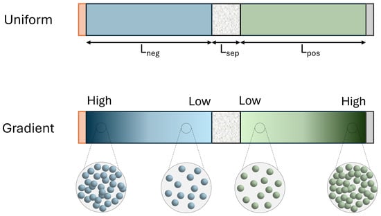
Figure 1.
Schematic representation of an LIB cell with uniform and gradient electrodes, where the uniform electrodes have constant porosity, compared to the gradient electrodes that have a varied porosity throughout their thickness.
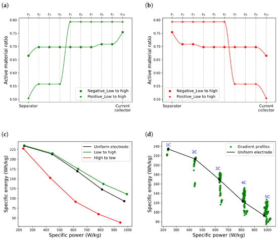
Figure 2.
Effect of the direction of the porosity gradient profile on energy density. (a) Profile with a low active material next to the separator, (b) profile with a high active material ratio next to the current collector, (c) comparison of the effect of the two profiles on energy density, (d) an example of the effect of gradient profiles on energy density with low active material next to the separator.
In Figure 2a, the active material distribution is considered to be the highest close to the current collectors; conversely, in Figure 2b, it is considered to be the highest close to the separator. Figure 2c illustrates the effect of these two profiles on the Ragone plots. While the first combination improves the Ragone plot, the second profile decreases the energy level significantly at all C-rates. However, not all the profiles with the right direction lead to an improved energy level. In Figure 2d, all the points are displayed with all the generated profiles with a low to high direction; however, there are some points that fall below the base energy level. It is also possible that a profile improves the energy at a high C-rate and reduces it at low C-rates. This indicates the need for optimization to find the best active material profile that can result in the highest improvement at all C-rates.
2.2. Neural Network Model Development
Artificial neural networks (ANNs) are data-driven algorithms modeled after the structure of biological neurons in the human brain [32]. These models comprise a network of interconnected neurons designed to learn complex patterns within a dataset [33]. A neural network consists of an input layer, an output layer, and one or more hidden layers. When a network contains two or more hidden layers, it is referred to as a deep neural network (DNN) [34]. ANNs are versatile tools applicable to both supervised and unsupervised learning, as well as classification and regression tasks.
In a neural network (NN) model, information is transmitted from the input layer to the hidden layers through weight coefficients, bias terms, and activation functions. [35]. The weights show the importance of each feature, the bias is the intercept, and the activation function is a mathematical equation that adds non-linearity to the model, therefore enabling it to capture patterns. The weights and biases are randomly selected initially and then adjusted during the training procedure to minimize a loss function, defined as the discrepancy between the model predictions and actual targets in regression tasks [36].
In the first hidden layer, a weighted sum of input features is passed through the activation function to produce the output of each neuron of the hidden layer. A weighted sum of these outputs is then be fed to the neurons of the next hidden layer to pass through the activation function of that layer and generate the inputs to the next hidden layer. This forward procedure continues until reaching the output layer.
The non-linear output of each hidden layer can be shown as and defined as
where , and are the weight matrix and bias term of the ith hidden layer, and the input layer is defined as . The final prediction of the NN can be shown as
where is the activation function of the output layer.
In this study, a feed-forward DNN was developed to map the porosity distributions and positive electrode thickness to the specific energy at each operating C-rate, as shown in Figure 3. The model was developed in Python using TensorFlow and Keras libraries. The inputs to the model include the following: 10 points from the porosity profiles of the positive electrode (), 10 points from the porosity profiles of the negative electrode (), average active material value of the positive and negative electrodes (), positive electrode thickness (), and C-rate (24 inputs). The specific energy is the target of the NN model. The reason for not considering power density as another target is that our analysis showed that the power density is primarily influenced by the C-rate rather than any other design parameter. Thus, regardless of variations in electrode thicknesses, average active material ratios, and gradient profiles, the power density would remain nearly constant at each C-rate. Considering that the C-rate is already considered as an input feature, considering the power density as a second target would be redundant.
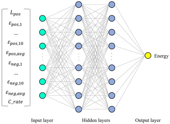
Figure 3.
Architecture of the NN used in this study, outlining the input features, input layer, hidden layers, and the specific energy prediction in the output layer.
The training dataset was generated using 11 profiles for each electrode (10 gradient and one constant) for thicknesses of = 120, 130, 140, 150, and 160 m; ; and an average active material of 0.7 and 0.65 for each electrode (overall resulting in 12,100 data points). Since the dataset was generated using a physics-based model, it did not contain outliers resulting from sensor errors, which are common in the measured data of experimental works. However, as shown in Figure 2, some profiles may cause a sudden drop in energy density at certain C-rates. These data points were not removed from the training dataset, and all the generated data were used for training the NN model. This approach allowed the model to learn how to discriminate the profiles that have the potential to increase the energy density level from those that lead to a reduction in energy density. A histogram of the train and test data is presented in Figure A3.
The model had two hidden layers, each with 1024 neurons and with the Sigmoid activation function for both hidden layers, defined as
and a linear activation function for the output layer. The train and test split ratio was (70:30) and 20% of the training data were kept for hold-out validation. Both stochastic gradient descent (SGD) and adaptive moment estimation (Adam) optimizers were tested for weight optimization. Similarly to SGD, the Adam optimizer also updates the weights, utilizing the gradient of the loss function. However, it also incorporates the first and second moments of the gradient to calculate an adaptive learning rate for each individual weight and bias [37]. This adaptive learning rate can lead to a more efficient training procedure and faster convergence [38]. Due to its superior performance during training, the Adam optimizer was used as the final optimization method for the model. The dropout method was employed as the regularization technique to prevent overfitting. This method was applied to both the first and second hidden layers with different rates. Through this experimentation, it was observed that implementing this method solely on the first hidden layer and with a rate of 0.5 yielded better performance compared to the other configurations. The model had a sufficiently complex structure, was trained for a considerable number of epochs, and utilized an adaptive learning rate through the Adam optimizer. These methods were implemented to mitigate the occurrence of underfitting (Table 3).

Table 3.
Summary of the structure of the NN model and utilized techniques.
The training history of the model is shown in Figure 4a by considering the mean squared error (MSE) as the loss function, defined as
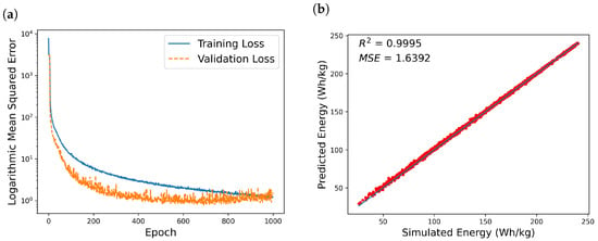
Figure 4.
The NN model performance plotted as the (a) loss history throughout 1000 epochs, and (b) the performance of the developed model on the test data. The blue line indicates the perfect fit ().
The MSE is a large value at the beginning of training (around 7000), but it quickly reduces to low values after the first few epochs (around 100 after 20 epochs) and then gradually decreases from then on. The MSE value is presented in a logarithmic scale to provide a clearer representation of the training process. Figure 4b shows the performance of the model on the test data, indicating the generalizability of the model to unseen data. The model’s generalizability is further tested in the next section by comparing the ML predictions to new porosity profiles with physics-based simulations of the electrochemical model.
3. Results
The developed NN model could quickly calculate the effect of the active material profiles on energy density within the selected range of positive electrode thicknesses at each C-rate. Therefore, a substantial dataset of candidate active material distributions was generated for four different case studies, where
- Case 1: and, ,
- Case 2: and, ,
- Case 3: and, ,
- Case 4: and,
In each case study, a total of 50 distinct profiles were generated for the positive and negative electrodes. The combination of these profiles yielded 2500 different combinations. The trained neural network systematically evaluated all 2500 combinations to determine the most optimal choice. The optimum choice was determined by finding the active material distributions for both electrodes that resulted in the greatest total energy difference. The energy difference at each C-rate is defined as
where is the specific energy of the jth profile combination () at ith C-rate () and is the energy density value of the same C-rate with the uniform electrodes, and is the difference caused by applying the profiles compared to the uniform electrode. The optimization criterion is defined as
where is the total summation of the energy difference for the jth profile combination, and the combination that yields the maximum value of is the frontier solution.
An exhaustive search was conducted across the entire design space, rather than employing a structured optimization method. This is because the NN model is highly efficient, allowing for rapid calculation of the effect of the candidate profiles. Furthermore, due to the random generation of the profiles, it was not possible to start the optimization procedure from a specific starting point in the design space and gradually move forward to achieve an optimum. A similar method was adopted in reference [27], demonstrating the reliability of such strategies.
When performing the optimization task, three of the profile combinations with the highest amount of total energy difference values were selected for five positive electrode thicknesses ( = 120, 130, 140, 150, and 160 m) in each case. The results indicated that some of the optimal distributions were common across the different thicknesses in each case. Therefore, it can be concluded that the optimal active material distribution profiles were independent of the electrode thickness and mostly related to the amount of average active material. Among all the distributions found for the five different thicknesses, two of the most repeated distributions were selected as the representatives of each case study. These distributions are shown in the Figure 5. The exact value of each point shown in Figure 5 is represented in Table A4 and Table A5 in Appendix B.
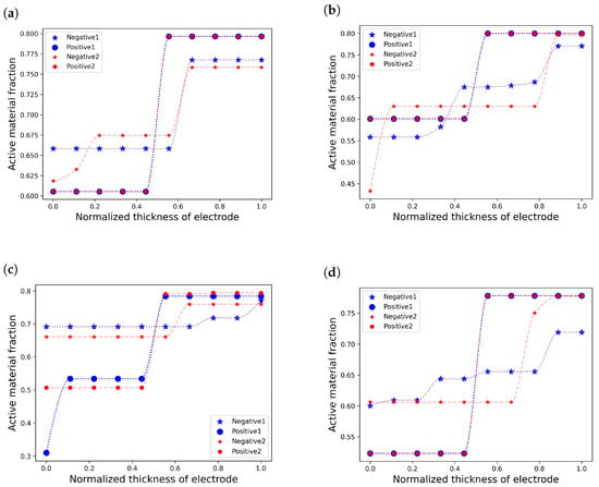
Figure 5.
The two most repeated distributions for all the selected electrode thicknesses in each case study. These case studies are (a) Case 1, (b) Case 2, (c) Case 3, and (d) Case 4.
The two representative distributions were then applied to the electrodes and the resulting Ragone plots were obtained from the physics-based model simulation, as can be seen in Figure 6. For the sake of simplicity, only three positive electrode thicknesses of 120, 140, and 160 m are shown in the figure.
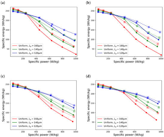
Figure 6.
Improved Ragone plots by applying the two selected distributions for C-rates between 0.2C and 5C for (a) Case 1, (b) Case 2, (c) Case 3, and (d) Case 4. Square and triangle symbols represent the effect of distribution number 1 and number 2, respectively.
The two distributions had a very close effect on all thicknesses for Case 1, while there was a slight difference between the resulting energy levels in the other cases, especially Case 3. It can be seen that the effect of gradient profiles was more obvious as the electrodes became thicker and as the C-rate increased. In order to demonstrate that the profiles did not result in an energy drop at lower C-rates, C-rates of 0.2C and 0.5C are also shown in the plots.
Table 4 shows the energy density at 5C in each case and the percentage improvement compared to the uniform electrodes. In Case 1 and Case 2, the theoretical capacity of the cells was equal for each positive electrode thickness. However, in Case 2, the average active material of the negative electrode was slightly lower than in Case 1. Consequently, the negative electrode thickness was higher to maintain the same electrode areal capacity based on Equation (5). This lower active material ratio yielded a higher relative improvement and also a higher energy density value across all the thicknesses. Comparing Case 3 and Case 4, it can be seen that a lower negative active material ratio also yielded a higher energy, but the percentage improvement was not necessarily higher. This shows that a slight reduction in the average active material ratio of the negative electrode, together with applying a profile, can be more helpful in enhancing the energy level, while having the same theoretical cell capacity.

Table 4.
Comparison of energy levels of gradient electrodes and uniform electrodes at 5C.
As can be seen from Figure 6, the power density was fairly consistent across the four different cases and electrode thicknesses at each C-rate. There was a slight difference between cases 1 and 2, compared to cases 3 and 4. This implies that the average active material ratio had a small impact on the power density. However, the disparity in power density among the three thicknesses was insignificant, indicating that the electrode thickness had minimal impact on the power density. For each electrode thickness and at each C-rate, the difference in power density between the uniform and gradient profiles was also negligible. The only obvious observed difference was for the thickness of 160 m at 5C for Case 1 and Case 2. This was due to an extremely short discharge time at these two points, leading to a small denominator in Equation (8). By applying the gradient profiles, the discharge time considerably increased, resulting in a small power density decrease, but a substantial energy density enhancement. For other thicknesses and C-rates, the power density difference between the uniform and gradient electrodes was insignificant. Given that during the optimization task, the focus was solely on the energy difference between the uniform and gradient electrodes, it can be concluded that disregarding the power density as a secondary objective was a valid assumption.
The effect of the gradient profiles on the capacity of the cell is represented in Figure 7. In all cases, the gradient profiles resulted in a higher deliverable capacity, and the improvement was clearer as the applied current was increased. In Case 1, a relative loss of 88.74% in capacity at 5C compared to the capacity at 1C was seen for the uniform electrodes. This relative capacity loss was 65.56% for the gradient electrodes. In Case 2, the capacity reduction was improved from 90.72% to 58.55%, showing a higher improvement compared to Case 1. The capacity improvement was also higher in Case 4 compared to Case 3, improving from 71.56% to 54.22% in Case 3, and from 66.09% to 46.41% in Case 4.
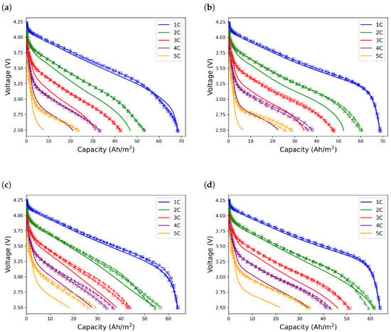
Figure 7.
Discharge voltage vs. cell capacity for C-rate between 1C and 5C for = 160 m considering (a) Case 1, (b) Case 2, (c) Case 3, and (d) Case 4. Square and triangle symbols represent the effect of distribution number 1 and number 2, respectively.
Figure 8 represents a comparison between the physics-based model simulations and NN predictions for the three most optimal distributions identified during the optimization process. The results indicate that the NN could predict the energy values with a high level of accuracy for all four case studies. However, the error was slightly higher for the cases where the positive electrode active material was 0.65, especially at lower energy levels (high C-rates). This could have been because, for thinner electrodes, the active material profiles generated very close energy levels; therefore, it would be more difficult for the NN model to learn the relations.
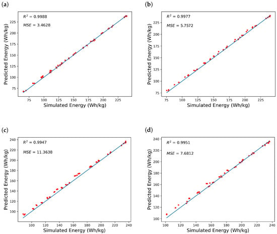
Figure 8.
Comparison of physics-based model simulations and NN predictions for (a) Case 1, (b) Case 2, (c) Case 3, and (d) Case 4. The blue line indicates the perfect fit ().
The primary benefit of using a NN as a substitute for electrochemical–thermal simulation for this optimization task is its low computational cost. The time required for each dataset (121 profiles, one thickness, and 5 C-rates) to be generated using the electrochemical–thermal model was about 2.5 h. Considering the same computational time, if the 2500 profiles were evaluated using the electrochemical–thermal model, the time required for calculation would have been about 2.15 days. Alternatively, the time required for the ML model to process the 2500 profiles was about 2 min. Therefore, if the parametric analysis for all thicknesses and four cases was directly performed using the physics-based model, it would have required about 43 days. In contrast, performing such an analysis using the NN model was completed in just 40 min. Since the ML model performed well on unseen datasets, it can be considered to be a viable option for such parametric analysis, making the calculations much lighter compared to the physics-based model simulation.
4. Conclusions
This study presented a NN surrogate model to investigate the impact of gradient active material profiles on the energy density of lithium-ion batteries. The model learned the relationship between the energy density and the profiles, electrode thickness, and C-rates by utilizing a dataset from an electrochemical–thermal model. The NN showed an accuracy comparable to that of the physics-based model, with a substantially reduced computation time, enabling it to evaluate a large number of profiles within minutes. Using this method, we investigated the relationship between electrode thicknesses and porosity profiles, and determined profiles that could cause energy improvement at 1C to 5C without reducing the energy at low C-rates. The efficiency of the NN model facilitated the optimization of the gradient profiles for both positive and negative electrodes across four different case studies. The randomly generated profiles provided a combination of layered and gradual variations in the active material throughout the electrodes’ thickness. This offered greater flexibility compared to the layered structures, enabling the generation of various profiles leading to a considerable energy density enhancement at high C-rates.
The drawback of this method is the need for a substantial dataset to train the NN model. Implementing ensemble methods or employing alternative machine learning techniques such as linear models, support vector machines, and Gaussian process regression, which usually perform better on small datasets could help resolve this issue.
The surrogate model could be used to investigate other optimization criteria, such as the highest energy at each C-rate and high energy at high C-rates, while allowing a certain energy decrease at lower C-rates. Furthermore, the surrogate model could be employed for inverse design applications, where a performance requirement is defined and then the thickness, porosity, and electrode structures can be optimized simultaneously.
Author Contributions
Conceptualization, M.N.A. and J.J.L.; methodology, M.N.A.; software, M.N.A.; validation, M.N.A. and J.J.L.; formal analysis, M.N.A. and J.J.L.; investigation, M.N.A.; resources, J.J.L.; data curation, M.N.A.; writing—original draft preparation, M.N.A.; writing—review and editing, O.S.B. and J.J.L.; visualization, M.N.A.; supervision, J.J.L.; project administration, J.J.L.; funding acquisition, J.J.L. All authors have read and agreed to the published version of the manuscript.
Funding
This research received no external funding.
Data Availability Statement
The original contributions presented in the study are included in the article, further inquiries can be directed to the corresponding author/s.
Acknowledgments
The authors would like to acknowledge Energy and Sensor Systems (ENERSENSE) group for academic support, and the Norwegian University of Science and Technology (NTNU) for PhD funding.
Conflicts of Interest
The authors declare no conflicts of interest.
Appendix A
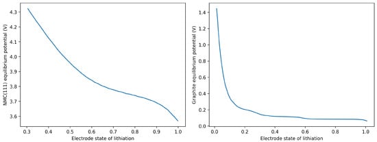
Figure A1.
Equilibrium potential vs. state of lithiation for positive and negative electrodes [39].
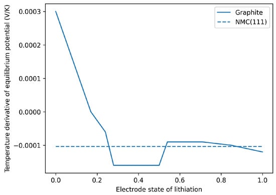
Figure A2.
Temperature derivative of equilibrium potential vs. state of lithiation for positive and negative electrodes, from COMSOL library.

Table A1.
Parameters used in the P2D model.
Table A1.
Parameters used in the P2D model.
| Property | Electrolyte/Separator | NMC(111) | |
|---|---|---|---|
| Separator thickness 1, (m) | - | 20 | - |
| Electrolyte volume fraction in separator 2, | |||
| - | 0.4 | - | |
| Binder volume fraction 1, | 0.1 | - | 0.1 |
| Particle radius 1, (m) | 8 | - | 5 |
| Bruggeman coefficient 1, p | 1.5 | 1.5 | 1.5 |
| Solid electrical conductivity 2, | |||
| 100 | - | 0.1 | |
| Solid diffusivity, | 3,4 | - | 3 |
| Max concentration in solid 3, | |||
| 31,507 | - | 49,000 | |
| Initial concentration in electrolyte 2, | |||
| - | 1200 | - | |
| Reaction rate constant 2, | |||
| - | |||
| Initial state of lithiation 5, | 0.89 | - | 0.25 |
| Final state of lithiation 5, | 0.022 | - | 0.728 |
| Electrolyte ionic conductivity 3, | |||
| Electrolyte diffusivity 3, | |||
| Molar activity 3, | |||
1 Assumed based on common values in the literature. 2 Reference [23]. 3 COMSOL material properties library. 4 Reference [25]. 5 Trial and error within the commonly used range in the literature was employed to set the open circuit voltage between 4.3 and 2.5 V.

Table A2.
Electrolyte-filled thermal properties of different cell parts [23].
Table A2.
Electrolyte-filled thermal properties of different cell parts [23].
| Property (Unit) | Negative Electrode | Separator | Positive Electrode |
|---|---|---|---|
| Heat capacity, | 1437 | 1978 | 900 |
| Thermal conductivity, | 5 | 1 | 5 |

Table A3.
Density values of cell parts [23].
Table A3.
Density values of cell parts [23].
| Cell Part | Density Value () |
|---|---|
| NMC111 | 4210 |
| Graphite | 2200 |
| Electrolyte | 1324 |
| Separator | 855 |
| Al current collector | 2707 |
| Cu current collector | 8954 |
| Binder and additive | 1800 |
Appendix B
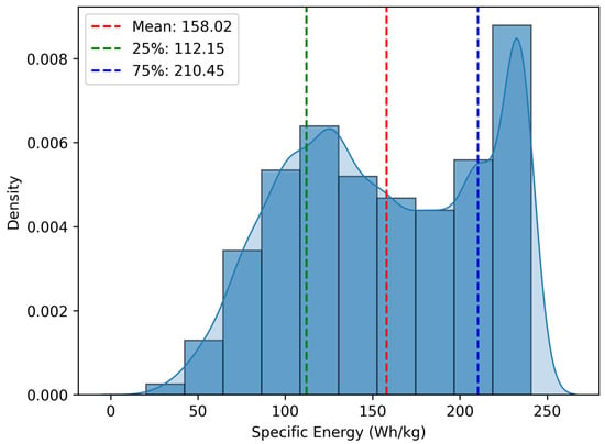
Figure A3.
Distribution of the train and test data.

Table A4.
Positive electrode points.
Table A4.
Positive electrode points.
| Case 1 | Case 2 | Case 3 | Case 4 | |||||
|---|---|---|---|---|---|---|---|---|
| Points | No. 1 | No. 2 | No. 1 | No. 2 | No. 1 | No. 2 | No. 1 | No. 2 |
| 0.6053 | 0.6053 | 0.601 | 0.601 | 0.3097 | 0.5069 | 0.5231 | 0.5231 | |
| 0.6053 | 0.6053 | 0.601 | 0.601 | 0.5339 | 0.5069 | 0.5231 | 0.5231 | |
| 0.6053 | 0.6053 | 0.601 | 0.601 | 0.5339 | 0.5069 | 0.5231 | 0.5231 | |
| 0.6053 | 0.6053 | 0.601 | 0.601 | 0.5339 | 0.5069 | 0.5231 | 0.5231 | |
| 0.6053 | 0.6053 | 0.601 | 0.601 | 0.5339 | 0.5069 | 0.5231 | 0.5231 | |
| 0.7966 | 0.7966 | 0.7999 | 0.7999 | 0.7837 | 0.7905 | 0.7783 | 0.7783 | |
| 0.7966 | 0.7966 | 0.7999 | 0.7999 | 0.7837 | 0.7905 | 0.7783 | 0.7783 | |
| 0.7966 | 0.7966 | 0.7999 | 0.7999 | 0.7837 | 0.7939 | 0.7783 | 0.7783 | |
| 0.7966 | 0.7966 | 0.7999 | 0.7999 | 0.7837 | 0.7939 | 0.7783 | 0.7783 | |
| 0.7966 | 0.7966 | 0.7999 | 0.7999 | 0.7837 | 0.7939 | 0.7783 | 0.7783 | |

Table A5.
Negative electrode points.
Table A5.
Negative electrode points.
| Case 1 | Case 2 | Case 3 | Case 4 | |||||
|---|---|---|---|---|---|---|---|---|
| Points | No. 1 | No. 2 | No. 1 | No. 2 | No. 1 | No. 2 | No. 1 | No. 2 |
| 0.6582 | 0.6183 | 0.5583 | 0.4329 | 0.6913 | 0.6608 | 0.6 | 0.606 | |
| 0.6582 | 0.6326 | 0.5583 | 0.6301 | 0.6913 | 0.6608 | 0.6091 | 0.606 | |
| 0.6582 | 0.6746 | 0.5583 | 0.6301 | 0.6913 | 0.6608 | 0.6091 | 0.606 | |
| 0.6582 | 0.6746 | 0.5823 | 0.6301 | 0.6913 | 0.6608 | 0.6437 | 0.606 | |
| 0.6582 | 0.6746 | 0.6749 | 0.6301 | 0.6913 | 0.6608 | 0.6437 | 0.606 | |
| 0.6582 | 0.6746 | 0.6749 | 0.6301 | 0.6913 | 0.6608 | 0.6554 | 0.606 | |
| 0.7675 | 0.7585 | 0.6785 | 0.6301 | 0.6913 | 0.7594 | 0.6554 | 0.606 | |
| 0.7675 | 0.7585 | 0.6865 | 0.6301 | 0.7181 | 0.7594 | 0.6554 | 0.7504 | |
| 0.7675 | 0.7585 | 0.7704 | 0.7963 | 0.7181 | 0.7594 | 0.7192 | 0.7772 | |
| 0.7675 | 0.7585 | 0.7704 | 0.7963 | 0.7703 | 0.7594 | 0.7192 | 0.7772 | |
References
- Khan, F.; Rasul, M.; Sayem, A.; Mandal, N. Design and optimization of lithium-ion battery as an efficient energy storage device for electric vehicles: A comprehensive review. J. Energy Storage 2023, 71, 108033. [Google Scholar] [CrossRef]
- Park, K.; Park, J.; Seong, W.; Yoon, K.; Hwang, T.; Ko, K.; Han, J.; Jaedong, Y.; Kang, K. Understanding capacity fading mechanism of thick electrodes for lithium-ion rechargeable batteries. J. Power Sources 2020, 468, 228369. [Google Scholar] [CrossRef]
- Gao, X.; Liu, X.; He, R.; Wang, M.; Xie, W.; Brandon, N.; Wu, B.; Ling, H.; Yang, S. Designed high-performance lithium-ion battery electrodes using a novel hybrid model-data driven approach. Energy Storage Mater. 2021, 36, 435–458. [Google Scholar] [CrossRef]
- Chen, Y.; Zhao, B.; Yang, Y.; Cao, A. Toward high-areal-capacity electrodes for lithium and sodium ion batteries. Adv. Energy Mater. 2022, 12, 2201834. [Google Scholar] [CrossRef]
- Zhang, X.; Ju, Z.; Zhu, Y.; Takeuchi, K.; Takeuchi, E.; Marschilok, A.; Yu, G. Multiscale understanding and architecture design of high energy/power lithium-ion battery electrodes. Adv. Energy Mater. 2021, 11, 2000808. [Google Scholar] [CrossRef]
- Appiah, W.; Park, J.; Song, S.; Byun, S.; Ryou, M.; Lee, Y. Design optimization of LiNi0.6Co0.2Mn0.2O2/graphite lithium-ion cells based on simulation and experimental data. J. Power Sources 2016, 319, 147–158. [Google Scholar] [CrossRef]
- Guo, W.; Sun, Z.; Vilsen, S.; Meng, J.; Stroe, D. Review of “grey box” lifetime modeling for lithium-ion battery: Combining physics and data-driven methods. J. Energy Storage 2022, 56, 105992. [Google Scholar] [CrossRef]
- Zhang, H.; Ren, D.; Ming, H.; Zhang, W.; Cao, G.; Liu, J.; Wang, L.; Song, J.; Qiu, J.; Wang, J.; et al. Digital Twin Enables Rational Design of Ultrahigh-Power Lithium-Ion Batteries. Adv. Energy Mater. 2023, 13, 2202660. [Google Scholar] [CrossRef]
- Liu, C.; Liu, L. Optimal design of Li-ion batteries through multi-physics modeling and multi-objective optimization. J. Electrochem. Soc. 2017, 164, E3254. [Google Scholar] [CrossRef]
- Xue, N.; Du, W.; Gupta, A.; Shyy, W.; Sastry, A.; Martins, J. Optimization of a single lithium-ion battery cell with a gradient-based algorithm. J. Electrochem. Soc. 2013, 160, A1071. [Google Scholar] [CrossRef]
- De, S.; Northrop, P.; Ramadesigan, V.; Subramanian, V. Model-based simultaneous optimization of multiple design parameters for lithium-ion batteries for maximization of energy density. J. Power Sources 2013, 227, 161–170. [Google Scholar] [CrossRef]
- Wu, J.; Ju, Z.; Zhang, X.; Marschilok, A.; Takeuchi, K.; Wang, H.; Takeuchi, E.; Yu, G. Gradient design for high-energy and high-power batteries. Adv. Mater. 2022, 34, 2202780. [Google Scholar] [CrossRef] [PubMed]
- Yang, J.; Li, Y.; Mijailovic, A.; Wang, G.; Xiong, J.; Mathew, K.; Lu, W.; Sheldon, B.; Wu, Q. Gradient porosity electrodes for fast charging lithium-ion batteries. J. Mater. Chem. 2022, 10, 12114–12124. [Google Scholar] [CrossRef]
- Liu, L.; Guan, P.; Liu, C. Experimental and simulation investigations of porosity graded cathodes in mitigating battery degradation of high voltage lithium-ion batteries. J. Electrochem. Soc. 2017, 164, A3163. [Google Scholar] [CrossRef]
- Cao, W.; Liu, M.; Song, W.; Li, Z.; Li, B.; Wang, P.; Fisher, A.; Niu, J.; Wang, F. Regulating Sodium Deposition Behavior by a Triple-Gradient Framework for High-Performance Sodium Metal Batteries. Adv. Sci. 2024, 11, 2402321. [Google Scholar] [CrossRef]
- Ramadesigan, V.; Methekar, R.; Latinwo, F.; Braatz, R.; Subramanian, V. Optimal porosity distribution for minimized ohmic drop across a porous electrode. J. Electrochem. Soc. 2010, 157, A1328. [Google Scholar] [CrossRef]
- Golmon, S.; Maute, K.; Dunn, M. Multiscale design optimization of lithium ion batteries using adjoint sensitivity analysis. Int. J. Numer. Methods Eng. 2012, 92, 475–494. [Google Scholar] [CrossRef]
- Hosseinzadeh, E.; Marco, J.; Jennings, P. The impact of multi-layered porosity distribution on the performance of a lithium ion battery. Appl. Math. Model. 2018, 61, 107–123. [Google Scholar] [CrossRef]
- Zhou, H.; Gao, L.; Li, Y.; Lyu, Y.; Guo, Z. Electrochemical performance of lithium-ion batteries with two-layer gradient electrode architectures. Electrochim. Acta 2024, 476, 143656. [Google Scholar] [CrossRef]
- Du, Z.; Wood, D.; Daniel, C.; Kalnaus, S.; Li, J. Understanding limiting factors in thick electrode performance as applied to high energy density Li-ion batteries. J. Appl. Electrochem. 2017, 47, 405–415. [Google Scholar] [CrossRef]
- Yu, R.; Li, P.; Wang, K.; Zhang, H. Numerical Investigation on the Impact of Linear Variation of Positive Electrode Porosity upon the Performance of Lithium-Ion Batteries. J. Electrochem. Soc. 2023, 170, 050502. [Google Scholar] [CrossRef]
- Amiri, M.; Håkansson, A.; Burheim, O.; Lamb, J. Lithium-ion battery digitalization: Combining physics-based models and machine learning. Renew. Sustain. Energy Rev. 2024, 200, 114577. [Google Scholar] [CrossRef]
- Wu, B.; Han, S.; Shin, K.; Lu, W. Application of artificial neural networks in design of lithium-ion batteries. J. Power Sources 2018, 395, 128–136. [Google Scholar] [CrossRef]
- Quartulli, M.; Gil, A.; Florez-Tapia, A.; Cereijo, P.; Ayerbe, E.; Olaizola, I. Ensemble surrogate models for fast LIB performance predictions. Energies 2021, 14, 4115. [Google Scholar] [CrossRef]
- Gao, T.; Lu, W. Physical model and machine learning enabled electrolyte channel design for fast charging. J. Electrochem. Soc. 2020, 167, 110519. [Google Scholar] [CrossRef]
- Sui, C.; Li, Y.; Li, X.; Higueros, G.; Wang, K.; Xie, W.; Hsu, P. Bio-Inspired Computational Design of Vascularized Electrodes for High-Performance Fast-Charging Batteries Optimized by Deep Learning. Adv. Energy Mater. 2022, 12, 2103044. [Google Scholar] [CrossRef]
- Miyamoto, K.; Broderick, S.; Rajan, K. Three-dimensional microbattery design via an automatic geometry generator and machine-learning-based performance simulator. Cell Rep. Phys. Sci. 2021, 2, 100504. [Google Scholar] [CrossRef]
- Bryntesen, S.N.; Strømman, A.H.; Tolstorebrov, I.; Shearing, P.R.; Lamb, J.J.; Burheim, O.S. Opportunities for the state-of-the-art production of lib electrodes—A review. Energies 2021, 14, 1406. [Google Scholar] [CrossRef]
- Bryntesen, S.N.; Finne, P.H.; Svensson, A.M.; Shearing, P.R.; Tolstik, N.; Sorokina, I.T.; Vinje, J.; Lamb, J.J.; Burheim, O.S. Structured aqueous processed lignin-based NMC cathodes for energy-dense LIBs with improved rate capability. J. Mater. Chem. A 2023, 11, 6483. [Google Scholar] [CrossRef]
- Chen, Z.; Danilov, D.; Eichel, R.; Notten, P. Porous electrode modeling and its applications to Li-ion batteries. Adv. Energy Mater. 2022, 12, 2201506. [Google Scholar] [CrossRef]
- Plett, G. Battery Management Systems, Volume I: Battery Modeling; Artech House: Norwood, MA, USA, 2015. [Google Scholar]
- Ren, Z.; Du, C. A review of machine learning state-of-charge and state-of-health estimation algorithms for lithium-ion batteries. Energy Rep. 2023, 9, 2993–3021. [Google Scholar] [CrossRef]
- Wei, Z.; He, Q.; Zhao, Y. Machine learning for battery research. J. Power Sources 2022, 549, 232125. [Google Scholar] [CrossRef]
- Gao, T.; Lu, W. Machine learning toward advanced energy storage devices and systems. Iscience 2021, 24, 101936. [Google Scholar] [CrossRef] [PubMed]
- Sui, X.; He, S.; Vilsen, S.; Meng, J.; Teodorescu, R.; Stroe, D. A review of non-probabilistic machine learning-based state of health estimation techniques for Lithium-ion battery. Appl. Energy 2021, 300, 117346. [Google Scholar] [CrossRef]
- Ye, J.; Xie, Q.; Lin, M.; Wu, J. A method for estimating the state of health of lithium-ion batteries based on physics-informed neural network. Energy 2024, 294, 130828. [Google Scholar] [CrossRef]
- Kinga, D.; Adam, J.B. A method for stochastic optimization. In Proceedings of the International Conference on Learning Representations, San Diego, CA, USA, 7–9 May 2015; Volume 5. [Google Scholar]
- Zhang, Z. Improved adam optimizer for deep neural networks. In Proceedings of the 2018 IEEE/ACM 26th International Symposium on Quality of Service (IWQoS), Banff, AB, Canada, 4–6 June 2018; pp. 1–2. [Google Scholar]
- Han, S.; Tang, Y.; Rahimian, S. A numerically efficient method of solving the full-order pseudo-2-dimensional (P2D) Li-ion cell model. J. Power Sources 2021, 490, 229571. [Google Scholar] [CrossRef]
Disclaimer/Publisher’s Note: The statements, opinions and data contained in all publications are solely those of the individual author(s) and contributor(s) and not of MDPI and/or the editor(s). MDPI and/or the editor(s) disclaim responsibility for any injury to people or property resulting from any ideas, methods, instructions or products referred to in the content. |
© 2024 by the authors. Licensee MDPI, Basel, Switzerland. This article is an open access article distributed under the terms and conditions of the Creative Commons Attribution (CC BY) license (https://creativecommons.org/licenses/by/4.0/).