Abstract
Revolutionary and cost-effective state estimation techniques are crucial for advancing lithium-ion battery technology, especially in mobile applications. Accurate prediction of battery state-of-health (SoH) enhances state-of-charge estimation while providing valuable insights into performance, second-life utility, and safety. While recent machine learning developments show promise in SoH estimation, this paper addresses two challenges. First, many existing approaches depend on predefined charge/discharge cycles with constant current/constant voltage profiles, which limits their suitability for real-world scenarios. Second, pure time series forecasting methods require prior knowledge of the battery’s lifespan in order to formulate predictions within the time series. Our novel hybrid approach overcomes these limitations by classifying the current aging state of the cell rather than tracking the SoH. This is accomplished by analyzing current pulses filtered from authentic drive cycles. Our innovative solution employs a Long Short-Term Memory-based neural network for SoH prediction based on residual capacity, making it well suited for online electric vehicle applications. By overcoming these challenges, our hybrid approach emerges as a reliable alternative for precise SoH estimation in electric vehicle batteries, marking a significant advancement in machine learning-based SoH estimation.
1. Introduction
As environmental pollution becomes a growing concern, electric vehicles are relying on energy storage solutions such as lithium-ion (Li-Ion) batteries for their high energy and power capabilities, low self-discharge rate, and eco-friendly attributes [1]. However, battery performance can deteriorate over time and with continuous use, leading to a decline in capacity and increased resistance. From now on, we referred to this as the battery’s state-of-health (SoH), which often exhibits nonlinear behavior over a battery’s lifetime due to accelerated degradation when undergoing stress conditions such as high temperatures or disregard of voltage and power limits. Assessing the SoH outside of a controlled laboratory setting poses a considerable challenge; various estimation techniques are explored in Section 2.2. Such techniques must be deployable on mobile battery management systems (BMS) in order to ensure vital information for vehicle safety and reliability.
The number of data-driven approaches present in the scientific literature has been skyrocketing recently thanks to their superior robustness, good estimation ability, and low computational cost. In the following sections, we aim to highlight significant contributions that have paved the way for this publication, followed by a summary showing the distinctive aspects of our study in comparison to the existing literature.
For comparability, many studies have used the National Aeronautics and Space Administration (NASA) Ames Prognostic Center of Excellence Li-Ion battery aging dataset for training, validation, or both. In this approach, batteries are exposed to three different current profiles: charge, discharge, and electrochemical impedance spectroscopy. For instance, Chang et al. (2021) established an online method utilizing fusion of incremental capacity and wavelet neural networks with genetic algorithm to estimate under discharge conditions [2]. Chai et al. (2022) proposed a method that uses empirical mode decomposition to reduce local fluctuations, an optimized dynamic single-exponential model to describe degradation, and a particle filter algorithm to determine the optimal system state. This method has shown good performance for one-step, multi-step, and long-term SoH estimation [3]. Jia et al. (2021) proposed a novel multi-scale model for predicting the SoH of Li-Ion batteries in order to improve accuracy and overcome the nonlinear fluctuations caused by temperature variation. Temperature data were analyzed in the frequency domain using wavelet packet transform and correlation analysis, while an estimation framework was developed using wavelet neural network and ensemble learning with an expectation maximization algorithm [4].
This study adopts a variant of the Long Short-Term Memory (LSTM)-based estimation method, similar to the approach employed by Lin et al. (2021), in which the authors utilized an LSTM-based network to create an aging estimation algorithm based on data from the charging process and capacity and a particle swarm optimization algorithm was used to optimize the LSTM model [5].
Outside the NASA dataset, there have been other LSTM based accomplishments as well; for instance, Shu et al. (2021) created a machine learning-based SoH estimation scheme for Li-Ion battery packs in order to overcome the high demand for training data. The charging duration for a predefined voltage range was used as a health feature, and an LSTM network and transfer learning were incorporated to create the cell mean model for SoH estimation with partial data. The LSTM model was then used as the cell difference model (CDM) to evaluate SoH inconsistencies among cells, while the minimum estimation value in the CDM was used to determine the pack’s SoH. The data used in their study consisted of a variation of constant current/constant voltage (CCCV) charging/discharging profiles of three different cell types [6]. Cheng et al. (2021) used an empirical mode decomposition (EMD) and backpropagation LSTM neural network, which relies on easily available battery parameters such as current and voltage to estimate the SoH, then processed the data through the EMD method to reduce the impact of capacity regeneration and other situations [7]. Kong et al. (2021) proposed a framework to predict SoH using a combination of a convolution neural network (CNN) and an LSTM. The CNN was used to extract aging characteristics from the raw data obtained during the constant current charging process in order to estimate the SoH, then the results were then sent to the LSTM. A Bayesian optimization algorithm was employed for hyperparameter tuning. In our study, we similarly utilize a Bayesian optimization algorithm to obtain the best hyperparameters for the neural networks. The results presented by Kong et al. show a low root mean square error for SoH estimation with this approach [8].
Another noteworthy accomplishment using a filter-based approach was presented in Zhou et al. (2019), where the authors aimed to create an online SoH estimation method for in-use Li-Ion batteries in electric vehicles by analyzing the charge cycles and not the actual drive cycles. Their method used an iterated extended Gaussian process regression with Kalman filter to incorporate battery data at both the macro- and micro-level time scales [9].
SoH estimation using partial charging has been gaining more and more traction recently. X. Feng et al. used a support vector machine to compare partial charging curves in order to quantify the SoH with high accuracy [10], while Z. Wei, H. Ruan, Y. Li, J. Li, C. Zhang, and H. He extracted health indicators from partial charging data and used an artificial neural network (ANN) for precise real-time SOH estimation [11].
In addition to the main contribution of this paper, we combine the efforts of other papers to avoid the following issues:
- We deliberately avoid CC or CCCV charge data, discharge data, or their combination; while a number of previous studies [12,13,14,15,16,17] have demonstrated notable success with such current profiles, we instead prioritize analyzing the voltage response to a given current profile or mapping the available capacity by counting charges. In this way, our algorithm aims to provide a deeper understanding of the battery’s health status.
- We deliberately limit the implementation of algorithms in our approach, relying instead on ANNs, feature scaling, and mean value calculations. In this regard, we acknowledge the noteworthy work of Luciani et al. (2022), which is closely related to the research presented in this study. Luciani et al. employed drive cycles to find the age of the storage system and analyzed the SoH by examining the voltage response to a corresponding current pulse. Luciani et al. utilized predefined pulse tests and extracted features as inputs for their ANN; in contrast, our work focuses on filtering out pulses from drive cycles, and solely relies on the information provided by the BMS. Additionally, our algorithm is specifically tailored for real-time applications, while Luciani et al. developed an offline algorithm in order to optimize mobile computing power consumption [18].
- In this study, we avoid impractical parameters such as cycle count due to our recognition of their limited utility in real-world applications; instead, we focus on inputs generated by a standard BMS.
In addition to meeting all of the previously mentioned criteria, the main contribution of this work lies in the introduction of a novel approach that eliminates the need for time series analysis. Instead of tracking SoH over time, our methodology involves filtering current pulses during drive cycles and analyzing the voltage response to determine the absolute SoH. As a result, our approach shifts from tracking of SoH to classification, representing a significant departure from conventional methodologies.
We begin with our materials and methods, presenting the essential background needed. Here, we introduce the data utilized and outline the strategy employed. Following this, we proceed to unveil our results, followed by a discussion. Finally, we draw conclusions to encapsulate the entirety of this work.
2. Materials and Methods
This section provides foundational concepts and offers a detailed account of the experimental procedures employed in this study.
2.1. Battery Technology
A battery system generally consists of an energy storage unit, an electronic monitoring system, and safety components. Depending on the field of use, the energy storage unit, made up of interconnected modules and cells, is at the heart of the system and provides the power needed for specific applications. This study uses single cells in order to provide a proof of concept. The electronic monitoring system is called a BMS, and oversees the operation of the battery. It typically includes a microcontroller, voltage and current sensors, and other components to monitor and control the systems operations. In addition, it performs state estimations to provide an assessment of the battery’s performance. The safety components, such as fuses, electrical contactors, and cooling components, work in tandem with the BMS to protect the battery from damage or overuse. In short, the BMS is the brain of a battery system, ensuring that it runs smoothly and efficiently [19]. Irreversible chemical process occurring during operation are the main cause of the battery’s degradation. However, external factors such as temperature and improper usage can accelerate this process. Low temperatures can lead to the formation of lithium plating on the anode, while high temperatures can cause damage to the cathode material and lead to an increased build-up of solid electrolyte interphase [20,21,22]. Another factor is disregard of the battery’s voltage limits and its operation outside of the recommended [23]. The is a measure of the rate at which a battery is charged or discharged. It is defined as the ratio of the current I flowing into or out of the battery to the nominal capacity of the battery, as follows:
Battery state estimation is the process of determining the state-of-charge (SoC), SoH, and other key parameters of a battery system based on measurements of voltage U, current I, temperature T, and other factors. The SoC is a measure of the amount of capacity stored in the battery, and is expressed as a percentage of the full capacity [24]. SoH is a crucial metric that provides insight into the overall health of the battery. The SoH can be determined based on the battery’s increasing internal resistance or diminished capacity volume. For this study, we exclusively concentrate on SoH based on the available capacity, denoted as . quantifies the battery’s current capacity in relation to its initial capacity at the beginning of its lifespan (BoL). It serves as a predictive indicator for the battery’s remaining capacity and future performance. The calculation of is carried out using the following equation:
where is the current capacity and is the capacity at BoL. When the end of life (EoL) criteria are reached, the battery or cell should be replaced and either be recycled or used for second-life applications. The following section provides a short overview of the main SoH estimation strategies.
2.2. SoH Estimation Algorithms
The primary methods for predicting SoH can be broadly divided into three categories: model-based methods, data-driven methods, and hybrid methods. This overview provides a summary of the key concepts, placing specific emphasis on data-driven methods.
2.2.1. Model-Based Methods
Model-based methods involve deconstructing or simplifying the complex chemical and physical processes that occur within the battery’s cells [25]. The majority of research in this area focuses on the following methods:
Equivalent Circuit Model method: This method neglects the chemical composition or reactions and relies on the electrical properties of the battery and controlled voltage sources. It employs resistors and capacitors to model polarization and self-discharge, providing a more accurate simulation; however, it demands a detailed assessment of the battery in order to set its initial parameters [26].
Electrochemical model method: This method encompasses diverse aging mechanisms, notably the formation of SEI. It provides an understanding of the microscopic physical and chemical processes within the battery; however, it demands in-depth knowledge of the individual battery cell [27]. Additionally, electrochemical impedance spectroscopy-based methods, which treat the battery cell as a circuit with resistors, capacitors, and inductance to generate a Nyquist diagram, are considered electrochemical models [28].
Mathematical model-based methods: The term “mathematical model” can encompass various interpretations, usually referring to models employing mathematical formulas. Notably, two distinct methods are empirical models and statistical models, with the latter often employing statistical random filtering algorithms to monitor battery degradation. Alternatively, probabilistic model-based methods rooted in probability theory offer another mathematical approach [25].
2.2.2. Data-Driven Methods
Data-driven models learn using a given dataset. They use the patterns and relationships of the input data x to make estimations or decisions on new unseen input data x. Data-driven models have three main advantages:
- They often outperform traditional rules-based models, as presented in Section 2.2.1.
- When the model has been trained, it requires minimal computational resources to make estimations, making it highly attractive for mobile and online applications.
- Their minimal parameterization requirements make data-driven models an ideal solution for a wide range of applications while reducing the level of expertise required for implementation and maintenance.
Data-driven models need to undergo a process called training, in which a set of training data that represent a known outcome or output , called the ground truth, is used to train the model so that it can learn the correlation between input x and output [29]. The Mean Squared Error (MSE) is used to quantify how well the model is able to approximate the relationship between the inputs x and outputs . A low MSE value indicates that the model has a good fit to the data, while a high MSE value suggests that the model has poor accuracy and requires further improvement. For the sake of clarity, we introduce the Root Mean Squared Error (RMSE). While not employed during training due to potential compromises in resolution, RMSE proves valuable in regression-type problems, providing a more straightforward and interpretable metric. During the training process, the model’s parameters are updated to minimize the MSE and improve its performance on the training data [30]. In this study, the MSE is calculated using the following equation:
with being a single data point. In this study we delve deeper into ANNs with a focus on recurrent neural networks, specifically on techniques for time series forecasting and LSTM architectures. ANNs are machine learning models that are inspired by the structure and function of the human brain. An ANN is composed of interconnected artificial neurons that process information, and can be trained to perform tasks such as pattern recognition and estimations. A time series forecast is an estimation of the future values of a time series based on its past values. The goal of time series forecasting is to use the historical data of a time series to predict its future values with . This involves the challenge of mapping a sequence to another sequence; if , it becomes the challenge of mapping a sequence to vector. LSTM neurons are cells that are controlled by gates capable of filtering important events in long sequences. This allows the network to retain information for longer periods of time, letting it handle input sequences with long-term dependencies [31].
2.2.3. Hybrid Methods
Hybrid methods combine the strengths of various techniques to achieve improved performance. These methods are characterized by their versatility, as they can combine similar and disparate methods to optimize the model parameters and thresholds using a combination of optimization algorithms. This approach can lead to a considerable enhancement of overall performance, making hybrid methods a powerful tool in any data scientist’s arsenal [25].
2.3. Data Collection
This section sheds light on the process of gathering and preparing the data for training and validation.
2.3.1. Battery Cells
The battery cells used in this study were LIB power cells (LP2714897-51Ah-BEV). The key specifications are summarized in Table 1.

Table 1.
Specifications of LIB LP2714897-51Ah-BEV power cells.
Data were collected for nine cells, which were kept under constant environmental conditions in climate chambers with assigned ambient temperatures (see Table 2).

Table 2.
Progression of the initial and current capacity of each cell along with the calculated with the method outlined in Equation (2).
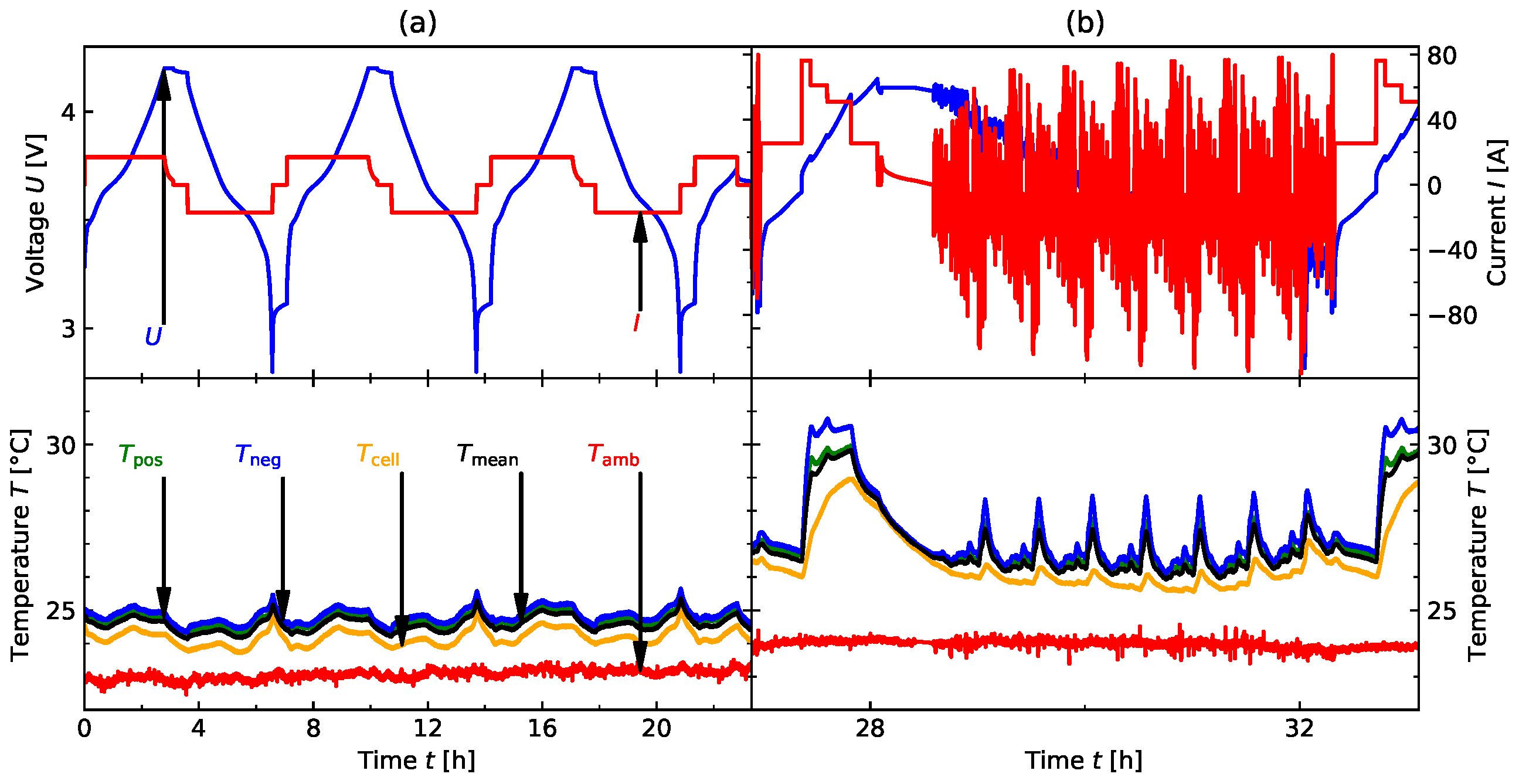
Four temperature sensors are assigned to each cell. One sensor is at a fixed point in the climate chamber without any direct contact with the cell. Its function is to record . The positive terminal (denoted by ) and negative terminal (denoted by ) are monitored by their corresponding sensors, with the sensor located at the center of the housing. It is noteworthy to highlight that during the model training process only was employed. This choice stemmed from practical considerations, as equipping every individual cell in a battery system with temperature sensors is not a viable option in real-world applications. Figure 1 shows the voltage, current, and temperature profiles for two selected examples. It can be seen that there is an offset among the sensors attached to the cell and . This is most likely due to the placement of the sensors in different locations in the climate chamber, as the temperatures , and are much more aligned with each other.
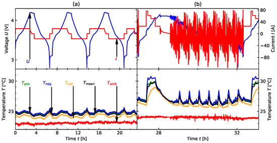
Figure 1.
Four diagrams featuring two examples of a single cell’s load performance. The first illustration, labeled (a), depicts a capacity check-up procedure and the second illustration, labeled (b), showcases ten drive cycles along with the corresponding charging cycles. The voltage U, current I, and all temperatures (, , , , and ) are displayed.
2.3.2. Method of Measurement
Each cell underwent the same experimental procedure. There was one BoL check-up and one EoL check-up when the cell has reached its EoL criterion. In the meantime, the cells were repeatedly cycled for 100 worldwide harmonized light vehicles test procedures (WLTP) at a specific temperature according to Table 2, followed by another capacity check-up. To ensure accuracy, each check-up at BoL, EoL, and after 100 WLTPs began by tempering the climate chamber to °C. The check-up process comprised a differential voltage analysis, a pulse test, an electrochemical impedance spectroscopy, and a capacity check. In this study, our focus is solely on the capacity check to determine . Figure 1 illustrates an example of one capacity check (in Figure 1a) and one drive cycle (in Figure 1b).
Figure 1a,b displays the voltage U, current I, and temperatures , , , and , as described in Section 2.3.2. is the average of the three temperatures at any given time step t. Figure 1a displays three CCCV cycles. Next, the cell was prepared for further procedures with SoC = 50%. To determine the available capacity, the mean of the charge and discharge cycles was taken. Table 2 lists the BoL capacities, current capacities, and calculated using Equation (2), which can help to understand the production variance among cells. The variation in the current available capacity was expected due to the ambient temperature , as per Table 2. Higher temperatures increase aging mechanisms, as described in Section 2.1. Figure 1b illustrates an example of the drive cycle, starting with 5 CC charging cycles at different potentials, followed by a 2 min break, another CC charge cycle, a CV charge cycle until the current I dropped C/20 of the charge, a 10 min break, and repeated WLTP cycles until SoC = 5%. The current profile considers higher-level operating limits, including the pulse concept and current limits. As a result, the current increases as the voltage decreases.
2.3.3. Data Preparation
The goal of this study was to develop a model that can be implemented on a standard BMS. To achieve this, the scope of available input parameters, denoted by x, was kept to a minimum. By analyzing the voltage U response to a corresponding current profile I, we aimed to determine the of each cell. To make the model viable for systems that do not come equipped with temperature sensors for each cell, we only rely on the ambient temperature . In addition, we cannot assume a steady flow of data points; this means that a time parameter providing the time period from one data point i to the last is provided. The output parameter is the value to be predicted by the model (). To summarize, the parameters available in this study are
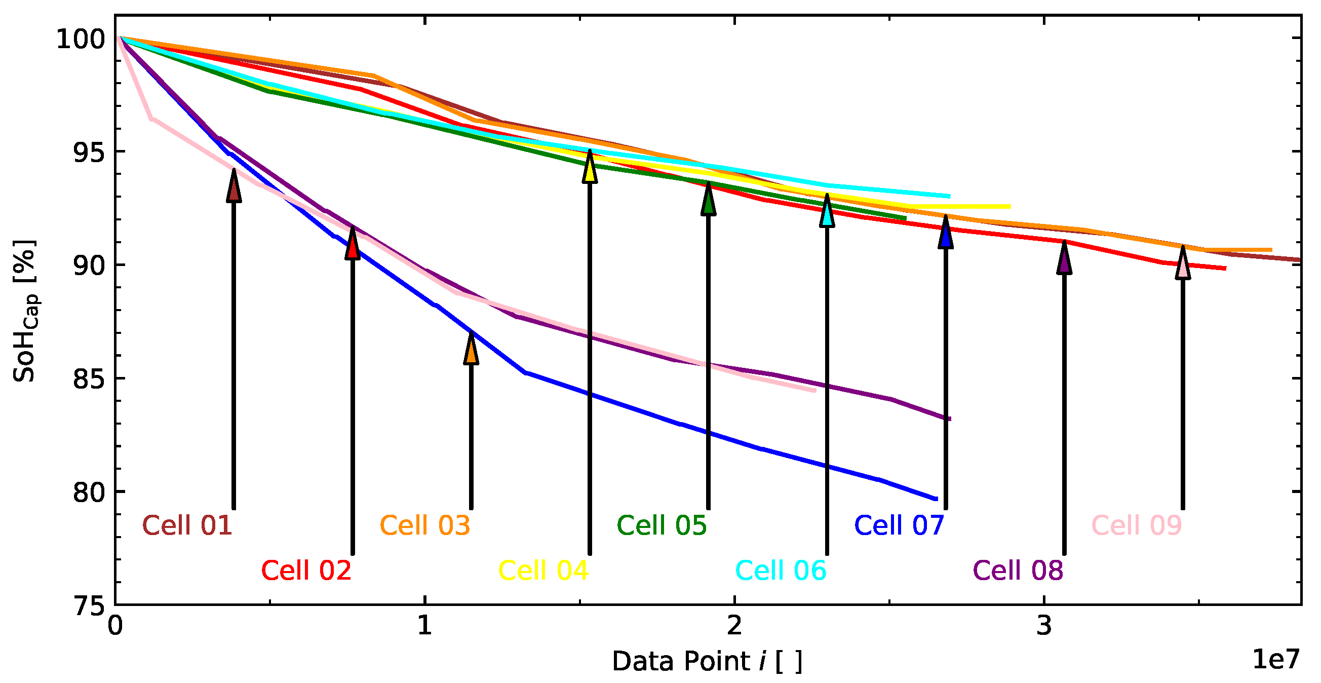
As detailed in Section 2.3.2, the was determined through periodic check-ups every 100 drive cycles. The data points were linearly interpolated between each check-up cycle. The plateaus visible between data points reflect the time elapsed before the next 100 drive cycles were initiated. Figure 2 illustrates the aging progression of each cell. For the sake of comparison, the figure displays over the recorded data points i rather than the time labels t. As a result, no plateaus are visible during periods when the cell was at rest.
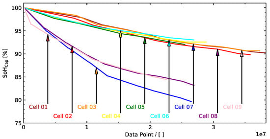
Figure 2.
for each of the nine cells plotted over the course of its lifespan.
The absence of capacity regeneration processes suggests that the periodic check-ups are appropriately spaced and the drive cycles have a significant impact on the degradation of the cell’s health [32]. The parameters U, , , and were scaled to the range [0, 1] using Equation (5), with being the scaled value at data point i and the unscaled value at data point i. The I parameter requires a larger range to distinguish between no load and low-level values. For instance, means that there is no load on the cell (the cell is relaxing), while is plainly another temperature; therefore, I is scaled by Equation (6). Table 3 provides all of the information regarding the scaling process.

Table 3.
The minima (low) and maxima (high) of each input and output parameter across all nine cells under . The actual values used to scale the data are under .
The variable x represents all input and output parameters. The parameter indicates the maximum and minimum values for each parameter, while represents the specific scaling values applied in the current study. The scale parameter was deliberately set to a smaller value compared to in order to accommodate the majority of values, which were less than 1 s in 99.974% of cases, while was set to Ah to ensure that the range of the cell with the lowest could easily reach = 80%, as ANNs are not able to work with values outside of the predetermined scaling parameters.
2.4. Realization of the SoH Model
This section delves into the methods used to develop and enhance the SoH model.
2.4.1. Strategy
The objective of this study was to evaluate the voltage response at different points in the lifespan of a cell under operating conditions using a current pulse. Our proposed approach is termed a “hybrid approach”, as it deviates from conventional time series forecasting and classification problems. Instead of using the entire time series data stream to the ANN analysis, we employed a filtering equation to isolate and analyze specific current pulses. Subsequently, a focused time window surrounding each identified pulse was selected and treated as an independent time series. The current pulses occur naturally during drive cycles, not as a result of a separate testing procedure. To accurately analyze the current data, the following filtering equation was employed:
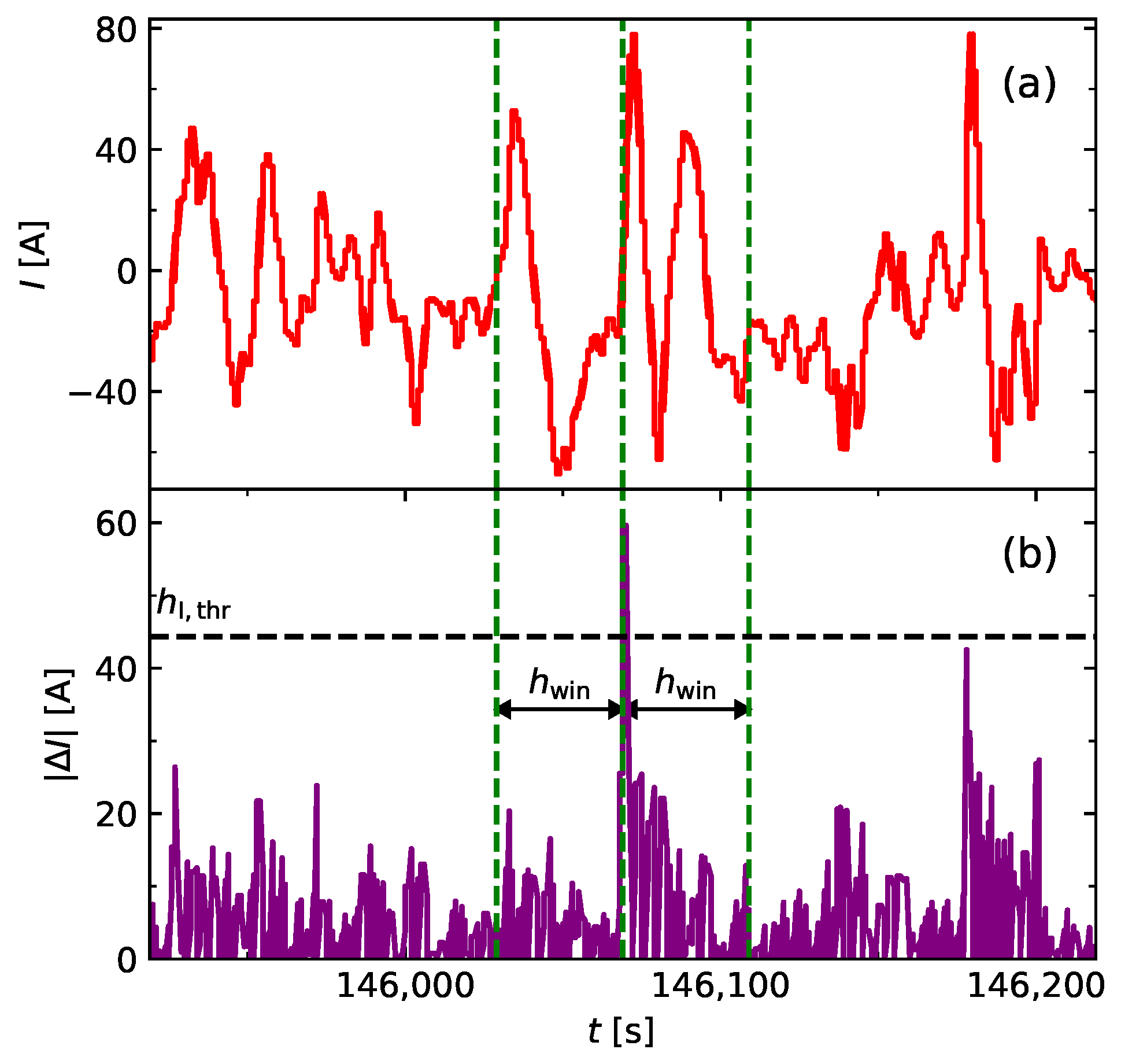
where is the value at data point i, is the value at data point , and is defined as . A data point i is filtered out of a drive cycle when , with being a threshold parameter. Subsequently, a time frame around i is selected according to the window size . The time frame has a range of . In Section 3.1 we investigate the values of and , with an example visualization presented in Figure 3.
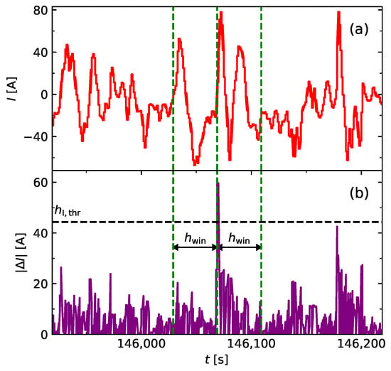
Figure 3.
Example showing an extract of a current profile of cell 1 in (a) and the corresponding absolute value of as calculated with Equation (7) in (b).
Figure 3a shows an extract of the current profile of a drive cycle from cell 1 picked at random, while Figure 3b shows the corresponding absolute value of as calculated with Equation (7). Hence, each input array has the following shape:
Another observation evident from the Figure 3 is that as the threshold decreases, the impact of the selected drive pattern diminishes. This is because the filtered current pulse exhibits increasingly less variance compared to current pulses from other drive patterns.
The ANN architecture comprises an input layer, multiple hidden layers () each containing numerous LSTM neurons (), and an output layer with a single dense neuron responsible for funneling all the information. The problem at hand deviates from traditional time series forecasting due to its complexity. Two key factors contribute to this classification discrepancy:
- As our aim was to demonstrate that an ANN can accurately determine the without prior knowledge of its SoH, the data were randomly shuffled before training and the states within each LSTM neuron were reset after each time frame was processed.
- Instead of analyzing a past output to predict a future output , we want to look at a past input to predict a future output . Thus, this is a sequence-to-vector or one-step estimation issue.
In this study, we used an Adaptive Moment Estimation (ADAM) optimization algorithm, which adaptively adjusts learning rates of various parameters based on past gradient information for faster convergence and better generalization performance of the model [33].
2.4.2. Hyperparameters
Hyperparameters (HP) are parameters that are determined ahead of the training process. The choice of HPs has a large impact on the model’s performance, and finding the optimal values requires experimentation, trial-and-error, or hybrid optimization approaches (see Section 3.1). The first two HPs ( and ) have already been mentioned in Section 2.4.1. The others concern the architecture of the ANN. First, the batch size was kept constant, which was for two reasons:
- A larger batch size results in a delayed response time before the ANN produces its initial estimation.
- A lower frequency of data processing by the training algorithm prior to the backpropagation process results in a less generalized model [34].
The number of iterations or epochs was limited by utilizing an early stopping approach, denoted as . Thus, if the training error did not show improvement after , the training process terminated automatically. The value of is closely related to the learning rate, regulated by the ADAM optimizer and represented as . To simplify the process, the early stopping HP was set to a constant value of during the HP optimization phase. The final two HPs are the number of neurons in each layer of the LSTM network, represented as , and the number of layers, represented as .
3. Results
This section provides a summary of this study’s findings, beginning with the results of the hyperparameter investigation followed by the presentation of the final SoH model.
3.1. Hyperparameter Optimization
To evaluate the models with individual HPs, a constrained global optimization package built upon Bayesian inference and the Gaussian process was used [35]. The first step is to initialize boundary conditions. This requires experiments in advance to gain an understanding of the architecture’s performance. Table 4 lists the lower limits of each HP in “min” and the upper limits in “max”. Next, the algorithm picks a random combination of HP values for steps in order to gain an understanding of the given search space. This is followed by a Bayesian update procedure for modifying the Gaussian process model at each new step for iterations, attempting to find the minimum value of an unknown high cost function in as few iterations as possible. To save time, only 80% of the data from cells 1, 4, and 7 were taken.

Table 4.
Boundary conditions and results of all HPs during the optimization process.
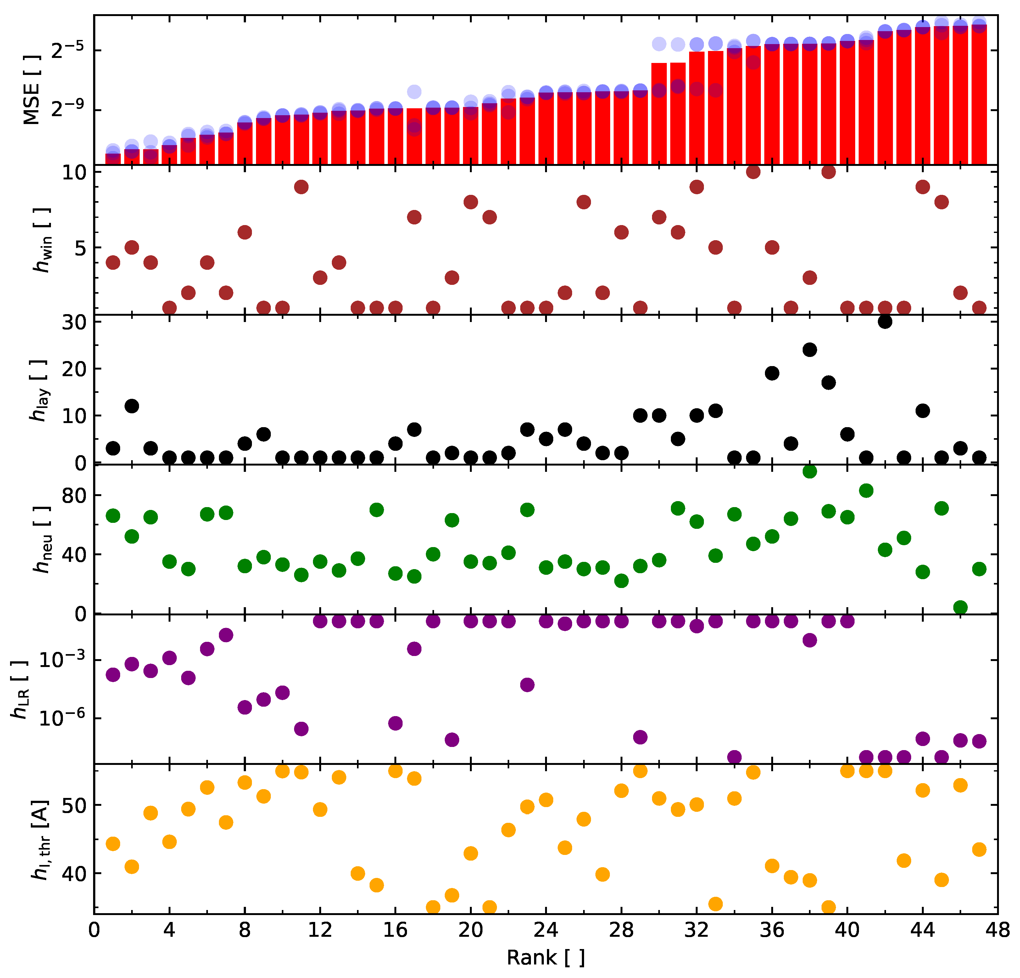
In this study, the process was initialized for steps and continued to run for an additional iterations. Due to the stochastic nature of ANNs, every iteration went through the training process three times and the arithmetic mean of the MSE was calculated. The results of this experiment are visualized in Figure 4.
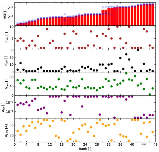
Figure 4.
Results of the Bayesian optimization process.
All six diagrams are ordered by rank (lowest rank = lowest MSE). The upper diagram shows the MSE of each rank. The arithmetical mean is represented by red bars, while the individual training process is represented by blue markers. The lower five diagrams show all of the HPs in question. It was expected to find the best results with a higher threshold ; however, a higher threshold reduces the amount of time frames, and consequently the amount of training data on which the ANN can be trained. Thus, it can be concluded that the ANNs with outperformed the ANNs with . Table 4 shows the rank 1 results of the experiment.
3.2. SoH Model
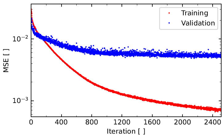
The ANN was modeled according to Section 2.4.1. Table 4 lists the values used to train and design the model with the full dataset, as described in Section 2.4.2. However, the parameter had to be adjusted to the amount of training data available. In addition, the early stopping parameter was set to . The metric used to train the model is the training loss. Therefore, the available data were split into training and validation data. Data for cells 3, 6, and 9 were reserved to validate the model. Thus, the training/validation split was 17/8. The MSE progression during training is shown in Figure 5.
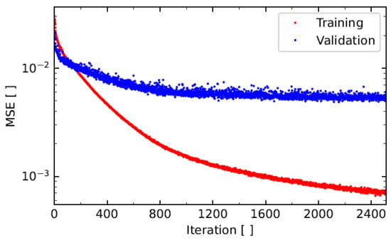
Figure 5.
Training and validation MSE progression over iteration.
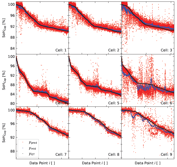
It can be seen that the MSE for the training and validation progresses do not drift apart; thus, no signs of overfitting are visible. The MSE for the training data significantly outperforms the validation MSE by multiple factors. This observation underscores the necessity of conducting a more thorough examination of . As more data points lacking beneficial value to the algorithm are present in the training process, the ANN tends to gravitate towards generating a look-up table rather than analyzing the voltage response. Consequently, the MSE trends begin to diverge. Despite successfully implementing an early stopping approach to mitigate notable overfitting, the noticeable difference in MSE suggests that an improved filtering method would enhance the effectiveness of this approach. The results are shown in Figure 6, where show the rescaled output of the ANN in comparison to the rescaled ground truth .

Figure 6.
The diagrams display the results of the algorithm applied to data points across all nine cells. These diagrams illustrate the comparison between the actual values , the predicted values , and the middle values .
The graphs depict the for each individual cell. The ground truth values, represented by , are the same as in Figure 2. Because the x-axis in all the subfigures is tailored to the BoL and the last recorded cycle, the numerical notation is not displayed here and can be found in Figure 2. The raw estimations, represented by , show a significant amount of noise. The noise in the data suggests that not all filtered current pulses provide the same quality of information to the ANN. Nevertheless, a discernible trend can be observed, which can be extracted with some additional processing on to create . Despite repeating WLTP multiple times, the noise does not exhibit any periodicity; hence, it can be concluded that the data do not suffer from overfitting, and instead reflect the response of the voltage to the corresponding current pulse. This reinforces the robustness of our analyses. To determine the actual of the battery cell and extract the underlying trend in the noise, we applied an averaging procedure; specifically, we computed the average over a range of data points for all data points i using the following equation:
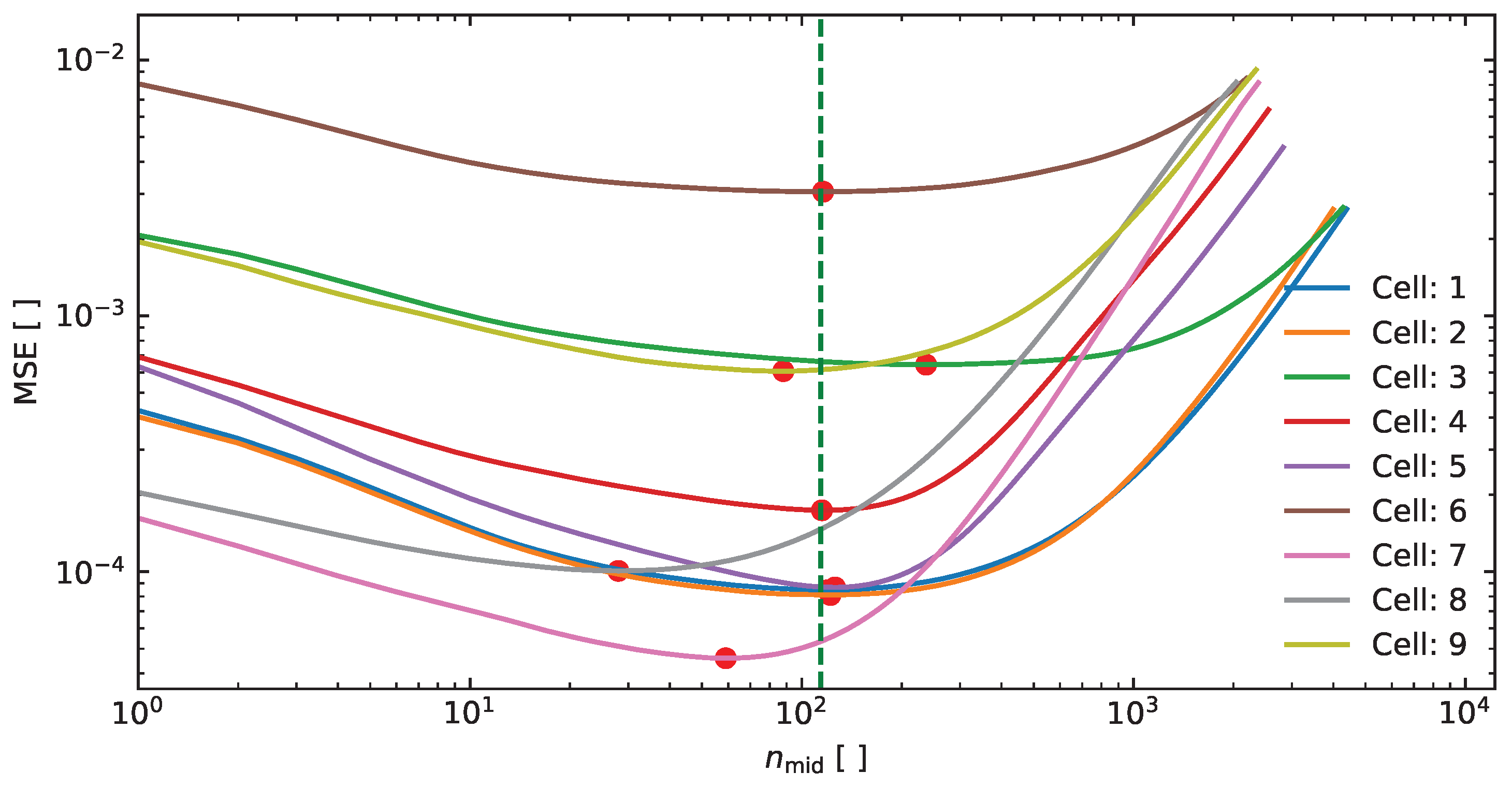
To find an appropriate value for , the MSEs for various values were calculated. The results are shown in Figure 7.
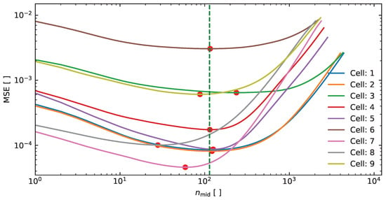
Figure 7.
Diagram displaying the MSE values of the middle estimation in relation to the corresponding middle value for each individual cell. The minimum MSE values are highlighted with a red dot, while a green line indicates the average minimum MSE across all cells.
The extrema for are marked with a red dot, and are not in tandem. The trade-off in this study is the value (green dashed line). Table 5 shows the MSE for , for the respective extrema, and the for . This yields a comprehensive average error of 1.84% across the entirety of the cells.

Table 5.
Table presenting the MSE results of the final trained model. The MSE column illustrates the MSE of the predicted values , the column displays the MSE of the middle estimations at their optimal middle value , and the column shows the MSE of the middle estimations when .
The visual results for are shown in Figure 6.
4. Discussion
To fully unleash the potential of this approach, a more robust pulse filter that effectively minimizes overall noise needs to be created, which could render the need for data smoothing obsolete. However, this would require an increased quantity of data with greater diversity.
5. Conclusions
A dataset comprising nine cells from three different temperature environments was created, including WLTP drive cycles and an extensive check-up procedure. The data were labeled with the corresponding for machine learning purposes. Current pulses were filtered from the WLTP drive cycles and a functioning LSTM-based ANN was developed to analyze the voltage response to set current pulses. The network was optimized using a Bayesian optimization algorithm to achieve a cost effective and rapid hyperparameter solution. This hybrid approach led to a tool for estimating . While the result produced some noise, this was smoothed out over 114 data points to improve accuracy. To the best of our knowledge, this is the first study to utilize drive cycles to filter pulses. The results were subsequently analyzed by an ANN for classification, thereby eliminating the need for any initialization process, tracking methods, or additional system information requirements. Furthermore, this study distinguishes itself by incorporating three key features. First, it requires no further computations beyond the ANN, feature scaling of input data, and data point averaging, none of which require expensive resources. Second, it provides a versatile approach for assessing > 76% at any stage of the cell’s lifecycle by analyzing the voltage response to a given current pulse, thereby eliminating the need for additional information. Third, it dispenses with the need for predefined CCCV profiles, which offers two benefits: the BMS does not need to rely on special or frequent events, and the probability of overfitting during training is reduced.
In Section 4, we have already highlighted the need for further investigation into the filter approach. Other potential outlooks for future work include:
- Expanding the model’s scope: moving beyond individual cells to modules and complete battery systems is crucial for performance testing.
- Considering alternative ANN methods: exploring convolutional and transformer-based neural networks could be beneficial, as LSTM approaches are known for their time-intensive training and computational costs.
- Diversifying the training dataset: incorporating a more varied dataset could offer a more comprehensive understanding of the approach’s potential. These strategic adjustments could contribute to a more nuanced exploration and application of the proposed model.
Author Contributions
M.K.: conceptualization, methodology, software, validation, formal analysis, investigation, writing—original draft, visualization. M.S.: writing—review and editing. A.F.: writing—review and editing, validation. K.P.B.: conceptualization, writing—review and editing, supervision, funding acquisition. All authors have read and agreed to the published version of the manuscript.
Funding
This work was supported by Bundesministerium für Wirtschaft und Energie (19l21014D).
Data Availability Statement
The data presented in this study are available on request from the corresponding author.
Acknowledgments
I would like to thank the Bundesministerium für Wirtschaft und Energie for financial resources and the project management organisation TÜV Rheinland Consulting GmBH. In addition, I would like to thank our project partners ElringKlinger AG and Huber Automotive AG.
Conflicts of Interest
The authors declare no conflicts of interest. The funders had no role in the design of the study, the collection, analysis, or interpretation of the data, the writing of the manuscript, or the decision to publish the results.
Abbreviations
The following abbreviations are used in this manuscript:
| Li-Ion | Lithium-Ion |
| SoH | State-of-Health |
| SoC | State-of-Charge |
| LSTM | Long Short-Term Memory |
| BMS | Battery Management System |
| NASA | National Aeronautics and Space Administration |
| CDM | Cell Difference Model |
| CCCV | Constant Current/Constant Voltage |
| CNN | Convolutional Neural Network |
| ANN | Artificial Neural Network |
| BoL | Beginning of Life |
| EoL | End of Life |
| MSE | Mean Square Error |
| RMSE | Root Mean Square Error |
| WLTP | Worldwide Harmonized Light Vehicles Test Procedure |
| ADAM | Adaptive Moment Estimation |
| HP | Hyperparameter |
References
- Peters, J.F.; Baumann, M.; Zimmermann, B.; Braun, J.; Weil, M. The environmental impact of Li-Ion batteries and the role of key parameters—A review. Renew. Sustain. Energy Rev. 2017, 67, 491–506. [Google Scholar] [CrossRef]
- Chang, C.; Wang, Q.; Jiang, J.; Wu, T. Lithium-ion battery state of health estimation using the incremental capacity and wavelet neural networks with genetic algorithm. J. Energy Storage 2021, 38, 102570. [Google Scholar] [CrossRef]
- Cai, L.; Lin, J.; Liao, X. A data-driven method for state of health prediction of lithium-ion batteries in a unified framework. J. Energy Storage 2022, 51, 104371. [Google Scholar] [CrossRef]
- Jia, J.; Wang, K.; Shi, Y.; Wen, J.; Pang, X.; Zeng, J. A multi-scale state of health prediction framework of lithium-ion batteries considering the temperature variation during battery discharge. J. Energy Storage 2021, 42, 103076. [Google Scholar] [CrossRef]
- Lin, J.; Yan, G.; Wang, C. Li-ion battery state of health Prediction based on Long Short-Term Memory Recurrent Neural Network. J. Phys. Conf. Ser. 2021, 2010, 012133. [Google Scholar] [CrossRef]
- Shu, X.; Shen, J.; Li, G.; Zhang, Y.; Chen, Z.; Liu, Y. A Flexible State-of-Health Prediction Scheme for Lithium-Ion Battery Packs with Long Short-Term Memory Network and Transfer Learning. IEEE Trans. Transp. Electrif. 2021, 7, 2238–2248. [Google Scholar] [CrossRef]
- Cheng, G.; Wang, X.; He, Y. Remaining useful life and state of health prediction for lithium batteries based on empirical mode decomposition and a long and short memory neural network. Energy 2021, 232, 121022. [Google Scholar] [CrossRef]
- Kong, D.; Wang, S.; Ping, P. State-of-health estimation and remaining useful life for lithium-ion battery based on deep learning with Bayesian hyperparameter optimization. Int. J. Energy Res. 2022, 46, 6081–6098. [Google Scholar] [CrossRef]
- Zhou, D.; Fu, P.; Yin, H.; Xie, W.; Feng, S. A Study of Online State-of-Health Estimation Method for In-Use Electric Vehicles Based on Charge Data. IEICE Trans. Inf. Syst. 2019, 102, 1302–1309. [Google Scholar] [CrossRef]
- Feng, X.; Weng, C.; He, X.; Han, X.; Lu, L.; Ren, D.; Ouyang, M. Online State-of-Health Estimation for Li-Ion Battery Using Partial Charging Segment Based on Support Vector Machine. IEEE Trans. Veh. Technol. 2019, 68, 8583–8592. [Google Scholar] [CrossRef]
- Wei, Z.; Ruan, H.; Li, Y.; Li, J.; Zhang, C.; He, H. Multistage State of Health Estimation of Lithium-Ion Battery with High Tolerance to Heavily Partial Charging. IEEE Trans. Power Electron. 2022, 37, 7432–7442. [Google Scholar] [CrossRef]
- Ruan, H.; Wei, Z.; Shang, W.; Wang, X.; He, H. Artificial Intelligence-based health diagnostic of Lithium-ion battery leveraging transient stage of constant current and constant voltage charging. Appl. Energy 2023, 336, 120751. [Google Scholar] [CrossRef]
- Manoharan, A.; Begum, K.M.; Aparow, V.R. Parallel Recurrent Artificial Neural Networks for Electric Vehicle Battery State of Health Estimation. In Proceedings of the 2022 17th International Conference on Control, Automation, Robotics and Vision (ICARCV), Singapore, 11–13 December 2022; pp. 590–595. [Google Scholar] [CrossRef]
- Zheng, W.; Bai, C.; Qiao, J.; Yin, H.; Fu, P. Research on Data-Driven-Based Remaining Useful Life of Lithium-ion Battery. In Proceedings of the 2022 International Conference on Sensing, Measurement and Data Analytics in the era of Artificial Intelligence (ICSMD), Harbin, China, 30 November–2 December 2022; pp. 1–6. [Google Scholar] [CrossRef]
- Hemdani, J.; Degaa, L.; Soltani, M.; Rizoug, N.; Telmoudi, A.J.; Chaari, A. Battery Lifetime Prediction via Neural Networks with Discharge Capacity and State of Health. Energies 2022, 15, 8558. [Google Scholar] [CrossRef]
- Falai, A.; Giuliacci, T.A.; Misul, D.A.; Anselma, P.G. Reducing the Computational Cost for Artificial Intelligence-Based Battery State-of-Health Estimation in Charging Events. Batteries 2022, 8, 209. [Google Scholar] [CrossRef]
- Sahoo, S.; Hariharan, K.; Agarwal, S.; Swernath, S.; Bharti, R.; Han, S.; Lee, S. Transfer learning based generalized framework for state of health estimation of Li-ion cells. Sci. Rep. 2022, 12, 13173. [Google Scholar] [CrossRef]
- Luciani, S.; Anselma, P.G.; Silvagni, M.; Bonfitto, A.; Tonoli, A. Enabling Rapid State of Health Offline Estimation of a 48V Lithium-Ion Battery Pack. In Proceedings of the 2022 IEEE Vehicle Power and Propulsion Conference (VPPC), Merced, CA, USA, 1–4 November 2022; pp. 1–6. [Google Scholar] [CrossRef]
- Wang, Y.; Tian, J.; Sun, Z.; Wang, L.; Xu, R.; Li, M.; Chen, Z. A comprehensive review of battery modeling and state estimation approaches for advanced battery management systems. Renew. Sustain. Energy Rev. 2020, 131, 110015. [Google Scholar] [CrossRef]
- Waldmann, T.; Wilka, M.; Kasper, M.; Fleischhammer, M.; Wohlfahrt-Mehrens, M. Temperature dependent ageing mechanisms in Lithium-ion batteries—A Post-Mortem study. J. Power Sources 2014, 262, 129–135. [Google Scholar] [CrossRef]
- Ma, S.; Jiang, M.; Tao, P.; Song, C.; Wu, J.; Wang, J.; Deng, T.; Shang, W. Temperature effect and thermal impact in lithium-ion batteries: A review. Prog. Nat. Sci. Mater. Int. 2018, 28, 653–666. [Google Scholar] [CrossRef]
- Kopp, M.; Ströbel, M.; Fill, A.; Pross-Brakhage, J.; Birke, K.P. Artificial Feature Extraction for Estimating State-of-Temperature in Lithium-Ion-Cells Using Various Long Short-Term Memory Architectures. Batteries 2022, 8, 36. [Google Scholar] [CrossRef]
- Kucinskis, G.; Bozorgchenani, M.; Feinauer, M.; Kasper, M.; Wohlfahrt-Mehrens, M.; Waldmann, T. Arrhenius plots for Li-ion battery ageing as a function of temperature, C-rate, and ageing state—An experimental study. J. Power Sources 2022, 549, 232129. [Google Scholar] [CrossRef]
- Sepasi, S.; Ghorbani, R.; Liaw, B.Y. Inline state of health estimation of lithium-ion batteries using state of charge calculation. J. Power Sources 2015, 299, 246–254. [Google Scholar] [CrossRef]
- Tian, H.; Qin, P.; Li, K.; Zhao, Z. A review of the state of health for lithium-ion batteries: Research status and suggestions. J. Clean. Prod. 2020, 261, 120813. [Google Scholar] [CrossRef]
- Li, Y.; Vilathgamuwa, M.; Farrell, T.; Choi, S.S.; Tran, N.T.; Teague, J. A physics-based distributed-parameter equivalent circuit model for lithium-ion batteries. Electrochim. Acta 2019, 299, 451–469. [Google Scholar] [CrossRef]
- Sankarasubramanian, S.; Krishnamurthy, B. A capacity fade model for lithium-ion batteries including diffusion and kinetics. Electrochim. Acta 2012, 70, 248–254. [Google Scholar] [CrossRef]
- Yao, L.; Xu, S.; Tang, A.; Zhou, F.; Hou, J.; Xiao, Y.; Fu, Z. A Review of Lithium-Ion Battery State of Health Estimation and Prediction Methods. World Electr. Veh. J. 2021, 12, 113. [Google Scholar] [CrossRef]
- Li, Y.; Liu, K.; Foley, A.M.; Zülke, A.; Berecibar, M.; Nanini-Maury, E.; Van Mierlo, J.; Hoster, H.E. Data-driven health estimation and lifetime prediction of lithium-ion batteries: A review. Renew. Sustain. Energy Rev. 2019, 113, 109254. [Google Scholar] [CrossRef]
- Goodfellow, I.; Bengio, Y.; Courville, A. Deep Learning; MIT Press: Cambridge, MA, USA, 2016; Available online: http://www.deeplearningbook.org (accessed on 15 May 2023).
- Graves, A. Long Short-Term Memory. In Supervised Sequence Labelling with Recurrent Neural Networks; Springer: Berlin/Heidelberg, Germany, 2012; pp. 37–45. [Google Scholar] [CrossRef]
- Meng, H.; Geng, M.; Xing, J.; Zio, E. A hybrid method for prognostics of lithium-ion batteries capacity considering regeneration phenomena. Energy 2022, 261, 125278. [Google Scholar] [CrossRef]
- Kingma, D.; Ba, J. Adam: A Method for Stochastic Optimization. arXiv 2014, arXiv:1412.6980. [Google Scholar]
- Smith, S.L.; Kindermans, P.J.; Ying, C.; Le, Q.V. Don’t Decay the Learning Rate, Increase the Batch Size. arXiv 2018, arXiv:1711.00489. [Google Scholar]
- Nogueira, F. Bayesian Optimization: Open Source Constrained Global Optimization Tool for Python. 2014. Available online: https://github.com/fmfn/BayesianOptimization (accessed on 15 May 2023).
Disclaimer/Publisher’s Note: The statements, opinions and data contained in all publications are solely those of the individual author(s) and contributor(s) and not of MDPI and/or the editor(s). MDPI and/or the editor(s) disclaim responsibility for any injury to people or property resulting from any ideas, methods, instructions or products referred to in the content. |
© 2024 by the authors. Licensee MDPI, Basel, Switzerland. This article is an open access article distributed under the terms and conditions of the Creative Commons Attribution (CC BY) license (https://creativecommons.org/licenses/by/4.0/).

