SOC Estimation of a Lithium-Ion Battery at Low Temperatures Based on a CNN-Transformer and SRUKF

Abstract

As environmental regulations become stricter, the advantages of pure electric vehicles over fuel vehicles are becoming more and more significant. Due to the uncertainty of the actual operating conditions of the vehicle, accurate estimation of the state-of-charge (SOC) of the power battery under multi-temperature scenarios plays an important role in guaranteeing the safety, economy, and reliability of electric vehicles. In this paper, a SOC estimation method based on the fusion of convolutional neural network-transformer (CNN-Transformer) and square root unscented Kalman filter (SRUKF) for lithium-ion batteries in low-temperature scenarios is proposed. First, the CNN-Transformer base model is established. Then, the SRUKF algorithm is used to update the state of the Coulomb counting method results based on the base model results. Finally, ensemble learning theory is applied to estimate SOC in multi-temperature scenarios. Data is obtained from laboratory conditions at −20 °C, −7 °C, and 0 °C. The experimental results show that the SOC estimation method proposed in this study is stable in terms of the root mean square error (RMSE) being between 2.69% and 4.22%. The proposed base model is also compared with the long short-term memory (LSTM) network and gated recurrent unit (GRU) network to demonstrate its relative advantages.

1. Introduction

With the increasingly serious global climate evolution problem, public awareness of reducing carbon footprints and protecting the environment has significantly increased [1,2,3]. Electric vehicles have gained widespread attention and gradually become an important trend in the field of transportation [4]. Lithium-ion batteries have been recognized as the main energy storage device for electric vehicles due to their high energy density, high charge/discharge efficiency, low self-discharge rate, long life, and high cycle stability [5,6]. Therefore, establishing a reliable battery management system (BMS) is important to monitor the battery’s operating status, ensuring the safe and stable operation of lithium-ion batteries [7]. However, the open-circuit voltage under different SOC is nonlinear and nonmonotonic, which makes it difficult to determine the SOC directly from the voltage. The key signals of the battery system will be subjected to noise interference due to the complexity of the actual operating conditions of the vehicle, and these interferences will affect the accuracy of the SOC estimation. At the same time, the battery will degrade during cyclic use, which will lead to an increase in the estimation error in the SOC estimation [8].

The following methods are currently utilized in the realm of battery SOC estimation: the Coulomb counting method, the open circuit voltage method, the model-based approach, and the data-driven technique [9].

The Coulomb counting method estimates the SOC of a battery by measuring the charge and discharge currents of the battery over a certain period of time and integrating them over time [10,11]. The advantage of this method is that it is relatively simple to implement and has a low cost. Ng [12] and Lee [13] proposed an enhanced Coulomb counting method for estimating the SOC and SOH of Li-ion batteries. The correction of operational efficiency and the evaluation of SOH are taken into account in the SOC estimation. Movassagh [14] formally derived and quantified the individual effects of four types of errors on the estimated SOC when applying the Coulomb counting method for SOC estimation and gave the corresponding treatment schemes. However, the Coulomb counting method also has obvious drawbacks, mainly the fact that the accuracy of the SOC estimation decreases with the time of use due to the accumulation of current measurement errors and the aging of the battery.

The open-circuit voltage method estimates the SOC by measuring the open-circuit voltage (OCV) of the battery at rest, which is based on a certain correspondence between the OCV and the SOC of the battery. The current value of SOC is determined by looking up the pre-established OCV–SOC mapping table or curve [15,16,17]. This method offers several benefits, including ease of use, reduced costs, and the capability to deliver high accuracy in the state-of-charge estimation once the battery has been fully recharged. Zheng [18] conducted small-current OCV and incremental OCV tests at three different temperatures, and the comparison results showed that the incremental OCV test method exhibited higher tracking accuracy. Fan [19] proposed an OCV–SOC curve identification method using current-voltage data without the need to measure or estimate the OCV. However, the disadvantage of the open-circuit voltage method is that it relies on the battery being able to reach a true open-circuit state, which is difficult to realize in practical applications.

The model-based strategy for estimating SOC involves simulating the battery’s electrochemical behavior by constructing a combination of one or more circuit elements, such as resistors or capacitors. Subsequently, the SOC is estimated using an observer following the system identification of the circuit model [20,21,22]. The advantage of this method is that it can better reflect the dynamic response of the battery under different operating conditions. Ma [23] proposed a multi-scale modeling method based on network hierarchy and an interactive network framework, which has a wide range of application scenarios. Mao [24] proposed a fusion model of an equivalent circuit model and a vector machine to enhance the SOC estimation at different temperatures. E.P [25] used an extended Kalman filter (EKF) algorithm based on the Thevenin model for SOC estimation and validated the SOC obtained in a vehicle dynamics model. However, the drawbacks of this approach are that the accuracy of the model depends on the quality of the parameter identification and the adequacy of the data. Complex models may lead to high computational effort.

The data-driven method to estimate SOC mainly relies on a large amount of battery operation data. It establishes a nonlinear relationship between battery operation data and SOC by learning the charging and discharging behavior and SOC change patterns from historical data [26,27,28]. The advantages of this approach include the ability to handle high-dimensional data, capture complex nonlinear relationships, and not be limited by battery physicochemical models [29,30]. Neural network models are often experimented with in combination with other methods to improve the accuracy and robustness of SOC estimation [31,32,33]. For example, Tian [34] and Fan [35] proposed a fusion method of the LSTM network with an augmented unscented Kalman filter (AUKF), Yang [36] and Wang [37] proposed a fusion method of the LSTM network with an unscented Kalman filter (UKF), and Liu [38] proposed a fusion method of the Backpropagation (BP) network with EKF, and the above fusion estimation algorithms have obtained good estimation results. Wu [39] utilized a support vector machine (SVM) to establish the relationship between SOC and V (voltage), I (current), and T (temperature). Experiments were conducted in nickel-metal hydride (NiMH) batteries, and the results showed that the proposed method has strong noise immunity. Wang [40] established a deep convolutional network for estimating battery SOC, with inputs of current and voltage. A Kalman filter was also constructed to fuse the SOC values that were calculated using the Coulomb counting method with those from the deep convolutional network, further enhancing the accuracy. However, a major limitation of the data-driven approach is its dependence on a substantial amount of labeled data for training, with the quality of the data directly impacting the model’s performance. The model’s generalization capabilities are contingent upon the variety and representativeness of the training dataset. Additionally, the model might not yield optimal results when dealing with aged batteries or under novel operating conditions. Furthermore, the complexity of the algorithm may lead to high computational costs and the model is poorly interpretive, which makes it difficult to intuitively understand its decision-making process.

In summary, in the field of SOC estimation for batteries, each method has its inherent limitations that can affect the accuracy and reliability of the estimation: The Coulomb counting method is fundamentally dependent on the precision of electric current measurement. Inaccuracies in the measurement of current can lead to cumulative errors in the SOC estimation. Additionally, this method requires a precise initial SOC value, which can be challenging to determine, especially in dynamic operating conditions. The model-based method’s effectiveness is heavily contingent upon the accurate identification of model parameters. If these parameters are not correctly identified, it can result in significant deviations in the SOC estimation. Furthermore, this method relies on simplified models that may not fully capture the complex electrochemical processes within the battery. This leads to estimation inaccuracies, especially under varying operating conditions and battery degradation over time. Data-driven methods show promise in terms of accuracy; however, they suffer from a lack of interpretability and are highly sensitive to the quality of the data used for training. These models can overfit the training data, leading to poor generalization when applied to new or unseen data. This sensitivity can result in a high number of estimation errors, particularly when the model encounters data that differs significantly from the training set. In order to solve the above problems, this paper proposes an SOC estimation method for lithium-ion batteries by combining a CNN-Transformer and SRUKF. Three measurable variables in the actual operation of the vehicle, V, I, and T, are selected as neural network inputs. First, a convolutional neural network is constructed for processing the raw data. It learns local features in the data through multiple convolutional layers and reduces the spatial dimension of the data through pooling operations. Further, the feature data processed through the convolutional neural network is inputted into the transformer encoder network, which utilizes its self-attention mechanism to capture the long-distance dependencies in the input data. In order to further reduce the estimation error, the SRUKF fuses the SOC value predicted by the neural network with that calculated by the Coulomb counting method. This method achieves the effect of smoothing the output. In addition, considering issues such as a slow electrochemical reaction rate and the unstable voltage response of batteries under low-temperature conditions, this article focuses on the research of SOC estimation in low-temperature environments. Experiments are conducted under three temperature scenarios −20 °C, −7 °C, and 0 °C. The ensemble learning theory is applied to obtain the SOC estimation under arbitrary temperature scenarios by linearly weighting the SOC results predicted by the constant temperature node model. The main research contributions of this paper are the following three aspects:

(1)

A CNN-Transformer network for SOC estimation is constructed, which combines the local spatiotemporal feature extraction ability of CNN and the long-range dependency capturing ability of the transformer. Good prediction results are obtained under different temperature datasets.

(2)

The SRUKF is implemented to integrate the predicted values from the neural network and the Coulomb counting method into the final forecast results. It mitigates the neural network’s propensity for excessive spikes during SOC estimation and rectifies the problems of cumulative offset error and high reliance on the accuracy of the current measurement inherent in the Coulomb counting method.

(3)

The application of ensemble learning theory involves combining the prediction results of multiple models to enhance overall estimation performance. The specific method is to linearly weight the SOC predictions from the fixed-temperature node models at −20 °C, −7 °C, and 0 °C to derive the SOC estimate for any low-temperature scenario. This allows the model to better handle the complex and variable environments of real-world applications.

The remaining chapters of this paper are organized as follows: Section 2 describes the methodology of this paper, including the CNN-Transformer algorithm, the resulting fusion process of the SRUKF and neural network, and how to apply the ensemble learning idea to achieve SOC estimation under multi-temperature scenarios. Section 3 describes the dataset used in this study as well as the experimental environment and the evaluation indexes setting. Section 4 shows the experimental results. Finally, Section 5 summarizes and outlines the paper.

2. Methodology

In this section, we describe the methodology proposed in this paper in detail. First, we introduce the CNN-Transformer network, where the CNN network is responsible for extracting features from the original data. Then, the data processed by the CNN network is inputted into the transformer network, which utilizes its self-attention mechanism to capture the long-distance dependencies in the input data. Next, we introduce the basic principle of SRUKF, along with the fusion process between the SRUKF and CNN-Transformer network. Finally, we introduce the proposed method of realizing the SOC estimation in multi-temperature scenarios based on the ensemble learning idea. The overall architecture diagram is shown in Figure 1.

2.1. CNN-Transformer

CNN is a deep learning algorithm, mainly used in the fields of image recognition, object detection, and computer vision [41,42]. The core idea of CNN is to use convolutional layers to automatically extract the features of the input data, and transform the original data into a series of representative feature quantities through continuous convolution, pooling, and other operations. These feature quantities can effectively represent the local structure and texture information in the original data, enabling the neural network to better recognize and understand the content in the original data. After acquiring the time series composed of V, I, and T, the local features are extracted by sliding the convolution kernel over the data and performing a point-by-point multiplication operation with the data, thus, extracting the local features. The convolution kernel can be viewed as a set of weighted parameters that are used to perform filtering operations on the input data. It will scan different regions of the data and generate a series of feature maps, where each feature map represents a different local feature. The specific process is shown in the following equation:

$$Y=ReLU(W\ast X+b)$$

(1)

Among them, $Y$ represents the output data, $X$ represents the input data, $\ast$ represents the convolution operation, $W$ represents the weight of the convolution kernel, $b$ represents the bias of each convolution kernel, and the values of $W$ and $b$ are calculated and updated through the Backpropagation process of the neural network.

The common pooling operations include max pooling and average pooling. In this paper, max pooling is used to retain the most significant features by selecting the maximum value in the local region as the pooling result. Let the dimension of the output $Y$ of the convolutional layer be $m\times n$, $m$ be the number of features, and $n$ be the dimension of features, and the specific processing is shown in the following equation:

$$P\left(i,j\right)=\underset{m^i}{\mathit{max}}Y\left(m_i,j\right)$$

(2)

Among them, $P\left(i,j\right)$ is the position value of the pooled features at positions $\left(i,j\right)$, where $i$ and $j$ represent the output height and width, respectively, and $m_i$ represents all features within the $i$-th window of the input features.

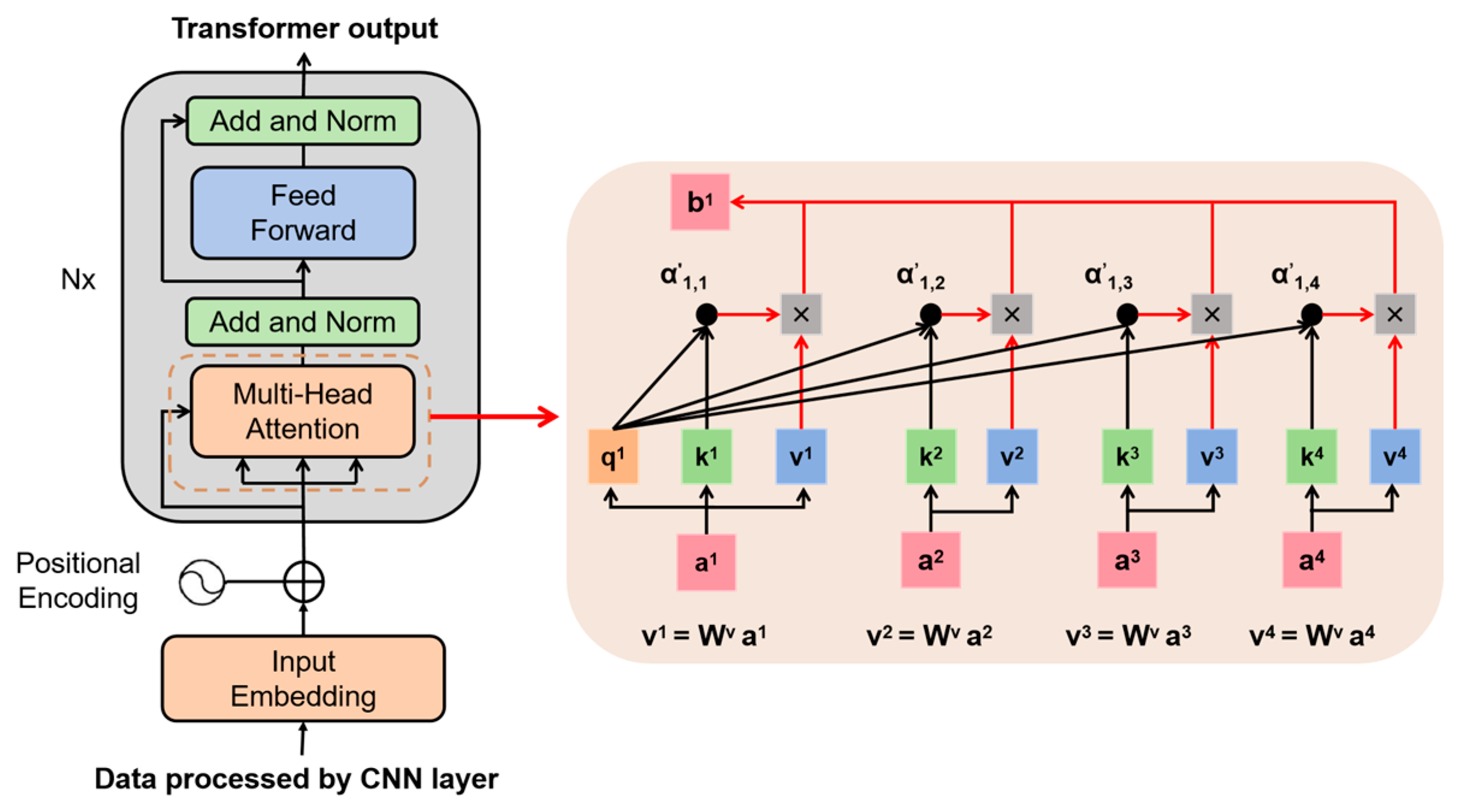
A transformer is a deep learning model based on the self-attention mechanism, and the core idea is to use the self-attention mechanism to weight each position in the input sequence to capture the relationships within the sequence. Different from traditional sequence models such as the recurrent neural network and long short-term memory network, the transformer adopts a parallel computational approach, which greatly improves the training speed and efficiency of the model. In the transformer model, the self-attention mechanism is realized by multi-head attention, the input sequence is divided into multiple heads, and each head pays attention to a different part of the sequence, thus, obtaining more comprehensive information. In addition, the transformer also introduces structures such as positional encoding and a feed-forward neural network to solve the position-dependent problems and nonlinear transformation requirements in the sequence model. In this paper, we only apply the encoder part of the transformer network, and its network structure diagram is shown in Figure 2. First, the array processed by the CNN is set to X, and is passed through the three different linear variations $W^Q$, $W^K$, and $W^V$ to obtain the values of Query, Key, and Value:

$$Q=X{W}^Q$$

(3)

$$K=X{W}^K$$

(4)

$$V=X{W}^V$$

(5)

Among them, $W^Q$, $W^K$, and $W^V$ are learnable parameters of the model.

Next, the process weight parameter is calculated for the self-attention mechanism.

$$Attention Weight=Attention\left(Q,K,V\right)=softmax\left({\displaystyle \frac{Q{K}^T}{\sqrt{d_k}}}\right)$$

(6)

where $d_k$ is the dimension of the input vector.

Finally, these weights are multiplied by the value V and the outputs of all heads are summed up to obtain the final self-attention output:

$$Output=Attention Weight\times V$$

(7)

The above is the calculation process of a single attention mechanism, and a multi-head attention mechanism processes information from multiple subspaces in parallel for multiple attention operations:

$$MultiHead\left(Q,K,V\right)=Concat\left(hea{d}_1, \dots , hea{d}_h\right)W^O$$

(8)

$$Hea{d}_i=Attention\left(Q{W}_i^Q,K{W}_i^K,V{W}_i^V\right)$$

(9)

where $W_i^Q$, $W_i^K$ and $W_i^V$ are the linear transformation matrices of queries, keys, and values, respectively. $W^O$ is the output weight matrix, and h is the number of attention heads.

The data after multi-attention processing is also fed into the fully connected feed-forward network, and these sublayers are connected to each other through residual connection and layer normalization, which will not be described more here, to finally obtain the output of the transformer network. The CNN-Transformer network constructed in this section serves as the measurement function for the Kalman filter, with input signals consisting of voltage, current, and temperature. The CNN component captures local features within these key parameters through convolutional and pooling layers. Compared to other neural networks such as traditional Feedforward Neural Networks (FNNs), Recurrent Neural Networks (RNNs), or GRU networks, the Transformer network does not rely on recurrent structures. Instead, it utilizes self-attention mechanisms to capture dependencies between all positions in the input sequence, regardless of how far apart two elements are in the sequence. This allows it to directly compute the relationship between any two elements, thereby better understanding the global context. Moreover, the parallel processing capability of the Transformer enables the more efficient utilization of hardware resources during training and inference, especially when dealing with long-sequence data. Therefore, using the CNN-Transformer network as the measurement function in the Kalman filter combines the strengths of CNNs in local feature extraction with those of Transformers in global information modeling. This approach enables the handling of both local and global information, enhancing the model’s generalization and accuracy. Such a combination allows the network to better understand and predict the dynamic behavior of batteries, particularly when processing battery data with temporal sequence characteristics. Furthermore, compared to other SOC estimation methods, the deep learning network built in this study does not rely on a single signal but instead captures the coupled features among the voltage, current, and temperature signals measured on the vehicle. This approach effectively avoids the issues of the flat voltage curve and OCV hysteresis that are present in traditional SOC estimation methods.

2.2. SRUKF

Kalman filtering is an optimal estimation algorithm. It enables the estimation of the state of a dynamic system from a sequence of measurement data containing noise. It is designed to solve estimation problems under linear dynamic systems and linear observation models [43,44]. SRUKF is an algorithm for the state estimation of nonlinear systems. It is an improvement of the traceless Kalman filter with the main objective of improving numerical stability. Although the state function and the measurement function constructed in this paper are linear functions, considering that the subsequent work will be extended to the joint estimation of multiple state quantities, to deal with possible nonlinear problems, the SRUKF algorithm will be used for the fusion of the results. The main idea of the SRUKF is to combine the estimated quantities of the state of the previous moment, the new system inputs, and the observation quantities, and to obtain the current time through the state transfer equation of the system state estimate of the system. Usually, the discrete state space equations for linear systems are:

$$x_{k+1}=A{x}_k+B{u}_k+{\omega }_k$$

(10)

$$y_k=C{x}_k+D{u}_k+v_k$$

(11)

where $x$ is the state variable, $y$ is the observation variable, and $A$, $B$, $C$, $D$ are the system matrices describing, respectively, the state transfer of the system, the effect of the control inputs on the state, the effect of the outputs on the state, and the effect of the control inputs on the outputs. ${\omega }_k$ and $v_k$ are the Gaussian white noises of the state variable $x$ and the observation variable $y$, whose variance matrices are, respectively:

$$\left\{\begin{array}{c}{Q}_w=E\left[{\omega }_k {\omega }_k^T\right]\\ R_v=E\left[v_k v_k^T\right]\end{array}\right.$$

(12)

When estimating the state of the system, the initial value of the state vector needs to be given in advance. The initial value of the state quantity is $x_0$, and the Cholesky decomposition factor of the covariance $P_0$ of the initial state estimation error is $s_0$:

$$S_0=chol\left(P_0\right)$$

(13)

The Cholesky decomposition factor $S$ of the mean $x$ and covariance $P$ of the state variable at each moment undergoes a traceless transformation to obtain 2n + 1 (n is the dimension of the state variable) sampling points (called the Sigma point set) with their weights $w$. The selection of the sigma point set is usually realized based on the correlation columns of the a priori mean and the square root of the a priori covariance matrix:

$$\left\{\begin{array}{c}{x}^0=\widehat{x}\\ x^i=\widehat{x}+\sqrt{n+\lambda }{S}^i, i=1, 2, \dots , n\\ x^i=\widehat{x}-\sqrt{n+\lambda }{S}^i, i=n+1,n+2, \dots , 2n\end{array}\right.$$

(14)

where $S^i$ is denoted as the i-th column of $S$. The sigma point set weights are calculated as:

$$\left\{\begin{array}{c}{\omega }_m^0={\displaystyle \frac{\lambda }{n+\lambda }}\\ {\omega }_c^0={\displaystyle \frac{\lambda }{n+\lambda }}+(1-{\alpha }^2+\beta )\\ {\omega }_m^i={\omega }_c^i={\displaystyle \frac{\lambda }{2\left(n+\lambda \right)}}, i=1, 2, \dots , 2n\end{array}\right.$$

(15)

where ${\omega }_m$ is the weight of the Sigma point set mean. ${\omega }_c$ is the weight of the covariance. The parameter $\lambda$ is a scaling ratio, which can reduce the total estimation error of the system. $\alpha$ is related to the state distribution of the sampling points, and $\alpha$ is usually set to a small positive value in order to reduce the influence of the higher-order moments. $\beta$ is a non-negative weight coefficient, which can reduce the peak error of the state estimation and improve the accuracy of the covariance.

The basic steps of the SRUKF algorithm are as follows:

(1)

The 2n + 1 sampling points and their corresponding weights are obtained using the traceless transform in Equations (14) and (15):

$$x_{k|k}^i=\left[{\widehat{x}}_{k|k},x_{k|k}^i+\sqrt{n+\lambda }{S}_k,{\widehat{x}}_{k|k}-\sqrt{n+\lambda }{S}_k\right]$$

(16)

(2)

The one-step prediction of these sampling points is calculated by the state transfer equation of the system:

$$x_{k+1|k}^i=f\left(x_{k|k}^i,u_k\right)$$

(17)

(3)

The one-step prediction of the state quantity is calculated from the one-step prediction of the Sigma point set and the weights of the Sigma point set $\omega$.

$${\widehat{x}}_{k+1|k}=\sum _{i=0}^{2n}{\omega }_m^i{x}_{k+1|k}^i$$

(18)

$$S_{xk}^{-}=qr\left(\sqrt{{\omega }_c^j}\left(x_{k+1|k}^i-{\widehat{x}}_{k+1|k}\right),\sqrt{Q_w}\right), j=1, 2, \dots , 2n,$$

(19)

(4)

From the one-step predictions of the Sigma point set and the system inputs, the 2n + 1 predictions of the system observations are computed through the system’s observation equations.

$$y_{k+1|k}^i=\sum _{i=0}^{2n}{\omega }_m^i{y}_{k+1|k}^i$$

(20)

(5)

The predicted values of the 2n + 1 observations are weighted and summed to obtain the predicted means of the observed variables of the system as well as the Cholesky factors of the covariances of the observed variables.

$${\widehat{y}}_{k+1|k}=chol\left(P_0\right)$$

(21)

$$S_{yk}^{-}=qr\left(\sqrt{{\omega }_c^j}\left(y_{k+1|k}^i-{\widehat{y}}_{k+1|k}\right),\sqrt{R_v}\right), j=1, 2, \dots , 2n,$$

(22)

$$S_{yk}=cholupdate\left(S_{yk}^{-},\left(y_{k+1|k}^0-{\widehat{y}}_{k+1|k}\right),{\omega }_c^0\right)$$

(23)

$$P_{xyk}=\sum _{i=0}^{2n}{\omega }_c^i\left[x_{k+1|k}^i-{\widehat{x}}_{k+1|k}\right]{\left[y_{k+1|k}^i-{\widehat{y}}_{k+1|k}\right]}^T$$

(24)

(6)

Calculate the Kalman gain matrix.

$$K_k=P_{xyk}{\left(S_{yk}{S}_{yk}^T\right)}^{-1}$$

(25)

(7)

Update using Kalman gain matrix.

$${\widehat{x}}_{k+1|k+1}={\widehat{x}}_{k+1|k}+K_k\left(y_{k+1}-{\widehat{y}}_{k+1|k}\right)$$

(26)

$$u_k=K_k{S}_{yk}$$

(27)

$$S_k=cholupdate\left(S_{xk},u_k,-1\right)$$

(28)

For SOC estimation, the state vector is $x=SOC$ and the Coulomb counting method is used to construct the state function. The measurement vector is the SOC output of the CNN-Transformer network. Therefore, the state space is modeled as follows:

$$SO{C}_k=SO{C}_{k-1}-{\displaystyle \frac{I_{k-1}\times ∆T}{C_n}}+\omega$$

(29)

$${Transformer}_k=SO{C}_k+v$$

(30)

where $I_k$ is the current at the k-th moment, $C_n$ is the nominal capacity of the battery, $\omega$ is the system noise, $\omega ~N\left(0,Q\right)$, and $v$ is the measurement noise, $v~N\left(0,R\right)$.

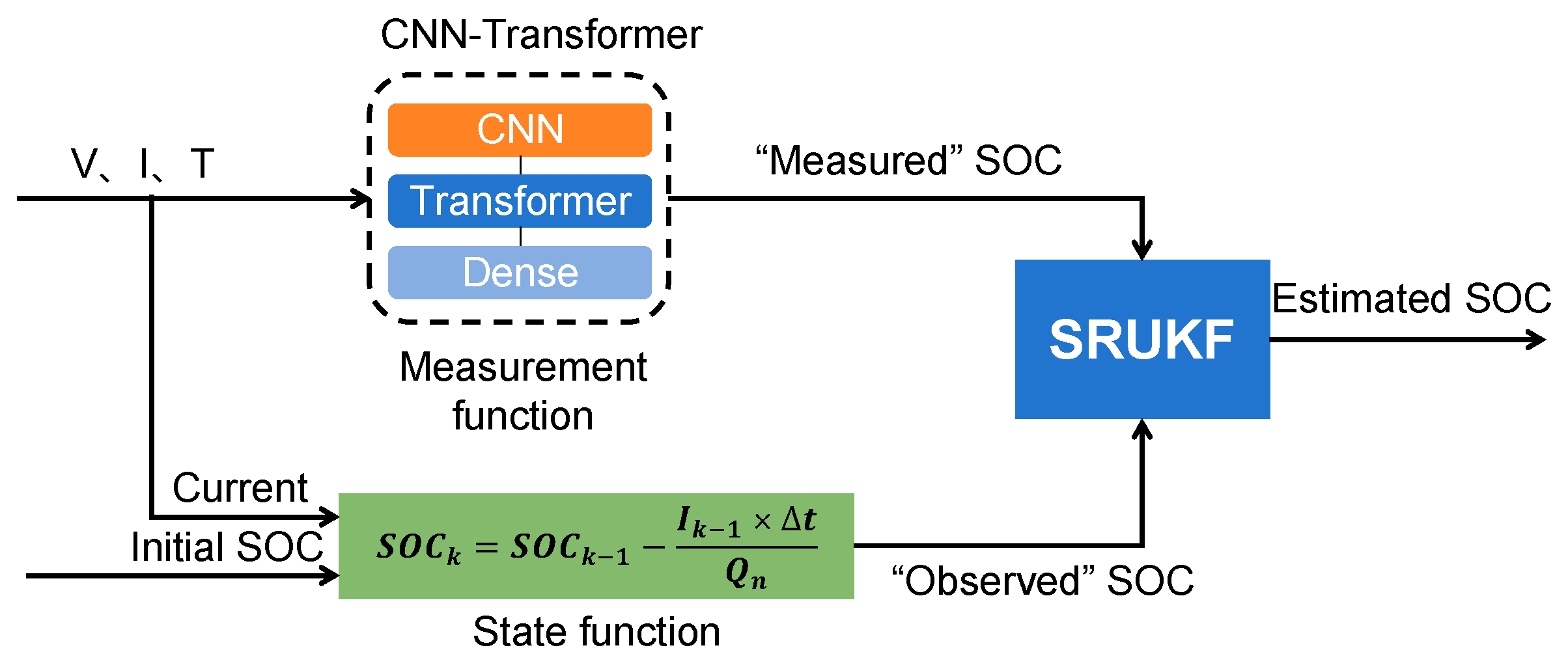
The framework is shown in Figure 3. The output of the transformer network is considered as the “measured” SOC, and the value obtained by the Coulomb counting method as the “observed” SOC. Using these two SOC values, the final SOC estimate is obtained by the SRUKF algorithm.

2.3. Ensemble Learning

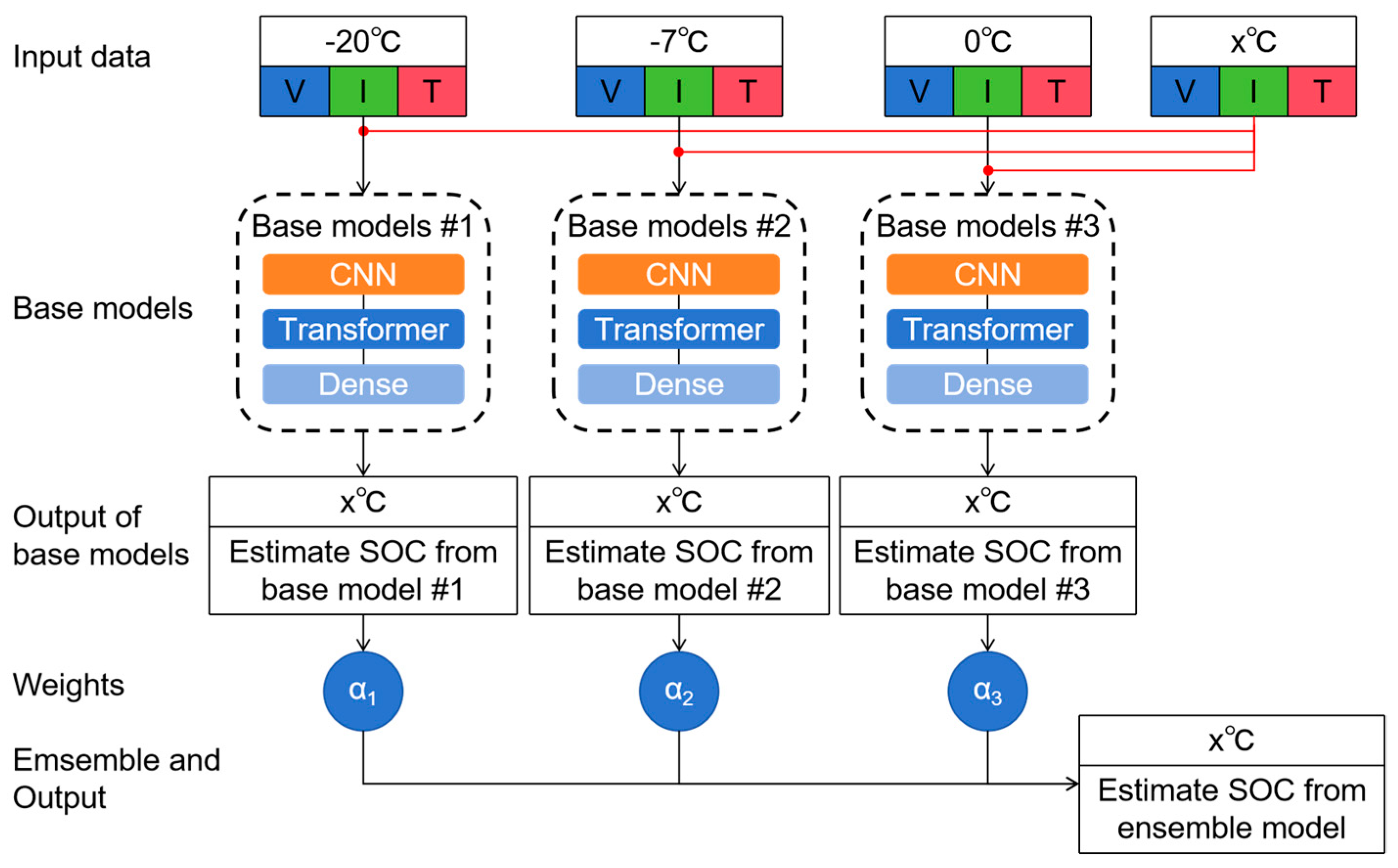
The core idea of ensemble learning is to construct a combined model with better performance by combining several basic learning models. Its main advantage is that it can significantly improve the performance and generalization ability of learning models. The model training is conducted at a specific temperature, but the actual operating conditions of the vehicle are variable. This study addresses the challenge of SOC estimation under varying temperature conditions. Employing the concept of ensemble learning, the SOC estimation under arbitrary temperature scenarios is obtained by linearly weighting the SOC results predicted by the fixed-temperature node model. The specific processing is shown in Figure 4, which includes three steps. The first step is the base model construction, with the lowest RMSE of the transformer at three temperatures as the standard retention. The second step is the weight determination, to determine the current distance from the three temperature points. Then, the three weight values determine and normalize the process. Finally, the weights of the four temperature calculation results are fused. The current temperature of the battery SOC is estimated to be x °C, and the base models are trained at −20 °C, −7 °C, and 0 °C, respectively. Then the weights b₁, b₂ and b₃, relative to the three base models at the current temperature node are calculated as follows:

$$b_1={\displaystyle \frac{1}{\left|a_1\right|}} b_2={\displaystyle \frac{1}{\left|a_2\right|}} b_3={\displaystyle \frac{1}{\left|a_3\right|}}$$

(31)

Then, the three calculated weight values are normalized to $c_1$, $c_2$, and $c_3$:

$$c_1={\displaystyle \frac{b_1}{b_1+b_2+b_3}} c_2={\displaystyle \frac{b_2}{b_1+b_2+b_3}} c_3={\displaystyle \frac{b_3}{b_1+b_2+b_3}}$$

(32)

Finally, the SOC estimation results under three temperature nodes are weighted and fused to obtain the SOC estimation value of the current temperature node $x$ °C:

$${SOC}_x=c_1{SOC}_{-20°\mathrm{C}}+c_2{SOC}_{-7°\mathrm{C}}+c_3{SOC}_{0°\mathrm{C}}$$

(33)

Among them, ${SOC}_{-20°\mathrm{C}}$, ${SOC}_{-7°\mathrm{C}}$, and ${SOC}_{0°\mathrm{C}}$ are the estimated SOC values in the models trained at three fixed temperature nodes, respectively.

3. Dataset Introduction and Experimental Setup

This section is divided into two parts; the first part will introduce the source of the dataset used in this paper and the process of acquiring the dataset, while the setup of the training set and the test set will be introduced. The second part will introduce the experimental scenarios as well as the hardware configurations, and finally give the evaluation indexes of the system.

3.1. Dataset Introduction

The battery type studied in this paper is a lithium iron phosphate battery. The research object is equipped as a whole battery pack rather than a battery monomer including two models, one large and one small. The large battery pack consists of large-capacity battery cells, and the small battery pack consists of small-capacity cells.

Table 1. Battery parameters table.

Technical Specifications	Values
positive electrode	Lithium iron phosphate
negative electrode	carbon
Nominal voltage	3.22 V
Pack A nominal capacity	133 Ah
Size of battery cell A (length × width × height) [mm]	220.3 × 44.5 × 112.2
Weight of battery cell A [kg]	2.380
Pack B nominal capacity	170 Ah
Size of battery cell B (length × width × height) [mm]	60.7 × 194.8 × 112.9
Weight of battery cell B [kg]	2.900

shows the basic parameters of the two battery monomers, which have the same electrical parameters except for cell capacity and size. The data acquisition process is carried out in the laboratory environment and the experimental scenario is shown in Figure 5. It is mainly composed of four parts: a liquid cooler, charging and discharging equipment, a data acquisition system, and a temperature box. The liquid cooler is used to cool down the battery, and its configuration is the same as that of the cooling system in the real vehicle. The charging and discharging equipment are used to provide and absorb the current for the battery. The data acquisition system is equipped with both data acquisition and charging/discharging control functions. The temperature box is used to control the ambient temperature where the battery is located. The experimental process is mainly divided into two parts, charging and discharging, and the key parameters of the charging and discharging process are shown in

Table 2. Key parameters table for the charging and discharging process.

Charge Test		Discharge Test
Key parameters	Values	Key parameters	Values
Charge test conditions	CW charge at 6.6 KW	Discharge test conditions	CLTC drive cycle
Charging cutoff voltage	3.65 V	Discharge cutoff voltage	2.0 V
Lower limit of allowable charging temperature	−20 °C	Lower limit of allowable discharge temperature	−30 °C
Allowed upper limit of charging temperature	55 °C	Maximum allowable discharge temperature	55 °C

. The charging process is carried out with a constant power of 6.6 KW, and the charging cutoff voltage is based on the single voltage reaching 3.65 V. The discharge process is performed with multiple China light-duty vehicle test cycles (CLTCs) to discharge the battery from a fully charged state, and the discharge cutoff voltage is based on the single voltage decreasing to 2.0 V.

There are two kinds of battery packs in this experiment, which are battery packs A and B. The nominal capacity of battery pack A is 133 Ah, and the nominal capacity of battery pack B is 170 Ah. There is no difference between the two kinds of battery packs except for the capacity, and the experimental conditions are also the same. The experimental process is shown in Figure 6. Firstly, the battery is put in a resting state and the temperature of the temperature box is adjusted to room temperature. Then, the battery is charged to full capacity with a constant power of 6.6 KW. Next, the temperature of the temperature box is adjusted to the target ambient temperature. Finally, the power condition discharge is carried out, and the data acquisition of other temperature scenarios is also referred to in the same process. In this paper, only the part of the discharge condition is extracted. The data sampling frequency is 1 s and the total length of the data is around 30,000 lines. The V, I, and T images of battery pack A and pack B at −20 °C, −7 °C, and 0 °C in the experimental process are shown in Figure 7. Different battery packs under different temperatures are all tested under CLTC conditions, and the discharge process of each battery pack from 100% to 0% SOC consists of 15 to 18 CLTC cycles. During the testing process, the test data of battery pack A is set as the training set and the test data of battery pack B is set as the validation set. In both the training and validation processes, data from the same temperature node are used.

3.2. Experimental Setup

This work uses the TensorFlow framework to build the whole network and calculates the network parameters using the Bayesian optimizer. The parameters available for optimization are batch size, sequence length, learning rate, number of multi-head attention layers, dropout rate, number of convolutional kernels, and convolutional kernel size. The parameters of the network calculated using the Bayesian optimizer are shown in

Table 3. Network parameter table.

Parameter	Value
Batch size	1672
Learning rate	0.00035
Number of convolutional kernels	20
Convolutional kernel size	120
Number of multi-head attention layers	2
Dropout rate	0.13

. The experiments are performed on a computer equipped with an Intel(R) Xeon(R) Gold 5120 CPU@2.20GH and NVIDIA TITAN GPU. This hardware resource simulates the cloud computing environment. The SOC estimation method constructed in this study can be deployed separately. The CNN-Transformer network is deployed in the cloud, and the Kalman filter is deployed on the vehicle. Model training and testing are conducted in the cloud, while result integration is performed on the vehicle. The hardware resources consumed by the Kalman filter are minimal, and the integration time is also at the millisecond level, thus, not affecting the timeliness of the SOC estimation.

The estimation performance of the proposed method is evaluated using the mean absolute error (MAE) and the RMSE criteria, which are defined as:

$$error={\left(SO{C}_k-SO{C}_k^{*}\right)}^2$$

(34)

$$MAE={\displaystyle \frac{1}{N}}\sum _{k=1}^N\left|SO{C}_k-SO{C}_k^{*}\right|$$

(35)

$$RMSE=\sqrt{{\displaystyle \frac{1}{N}}\sum _{k=1}^N{\left(SO{C}_k-SO{C}_k^{*}\right)}^2}$$

(36)

where $N$ is the number of samples, $SO{C}_k$ is the actual $SOC$ value at time k, and $SO{C}_k^{*}$ is the predicted value at time $k$.

4. Results and Discussion

In this section, the results are presented and discussed. In Section 4.1, in order to verify the accuracy and generalization of the proposed network, the CNN-Transformer model at −20 °C, −7 °C, and 0 °C were trained and validated. In Section 4.2, in order to verify the estimation effect of the SRUKF fused with the neural networks, the results of the CNN-Transformer network with the SRUKF are compared with the results of the CNN-Transformer without a filter. In Section 4.3, in order to verify the effect of ensemble learning, utilizing the idea of cross-validation to input the V, I, and T data under one of the temperature nodes into the models under the other two temperature nodes for prediction, the prediction results are linearly weighted to obtain the final prediction value. In Section 4.4, in order to verify the robustness of the SOC estimation algorithm proposed in this paper, experiments are carried out under 80% initial SOC and 60% initial SOC. Finally, in Section 4.5 in order to validate the advantages of the proposed network compared to other networks, the estimation results of the CNN-Transformer network are compared with those of other neural networks such as LSTM and GRU.

4.1. Base Model Training and Validation

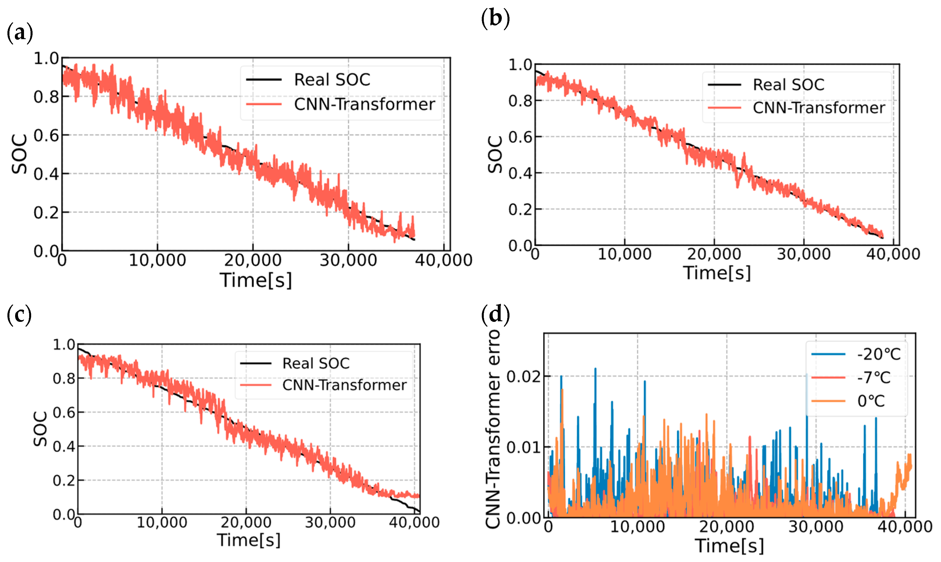
In this subsection, the CNN-Transformer model is evaluated at 0 °C, −7 °C, and −20 °C, respectively, and the train and test sets of the model at each temperature node are battery pack A and battery pack B, respectively. As shown in Figure 8a–c, they are the comparisons of the real SOC and the predicted SOC at 0 °C, −7 °C, and −20 °C, respectively, where the red lines are the predicted SOC values of the CNN-Transformer network and the black lines are the real SOC values. It can be seen that the predicted values of the neural network can track the real values in the overall trend. However, there are a lot of burrs in the details, which is due to the fact that the neural network is too sensitive when capturing the small fluctuations and high-frequency noises in the data. This leads to the overfitting phenomenon of the prediction results in the local area. The estimation error for each point at the three temperatures is shown in Figure 8d, where the blue line is the −20 °C error value, the red line is the −7 °C error value, and the orange line is the 0 °C error value. The overall values remain within 0.02, but the local fluctuations are very obvious, which is due to the fact that the output values of the neural network have more burr points, and the phenomenon is consistent with that shown in Figure 8a–c. The estimated overall RMSE and MAE are shown in

Table 4. RMSE and MAE values of the CNN-Transformer at −20 °C, −7 °C, and 0 °C.

Temperature (°C)	RMES (%)	MAE (%)
−20.	0.037327727	0.030301876
−7	0.026943953	0.020873434
0	0.042164227	0.03412065

. At −20 °C, the RMSE is 3.73% and the MAE is 3.03%. At −7 °C, the RMSE is 2.70% and the MAE is 2.09%. At 0 °C, the RMSE is 4.22% and the MAE is 3.41%. Overall, the RMSE and MAE can remain stable at around 3% at three temperatures.

4.2. Validation of SOC Estimation Results After SRUKF Filtering

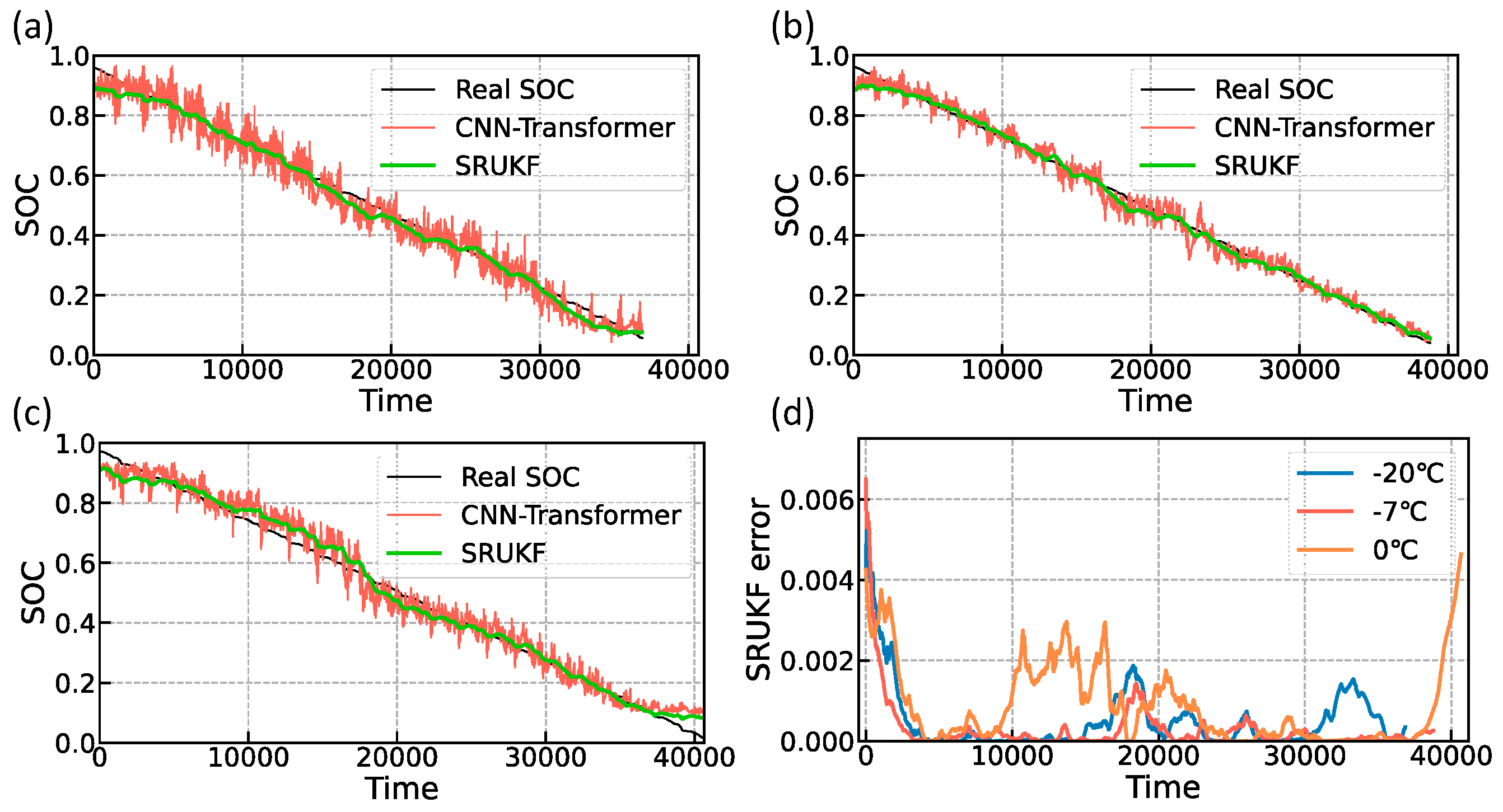
In this subsection, the SOC estimation method of CNN-Transformer-SRUKF proposed in this paper is compared with the CNN-Transformer method to validate the effectiveness of the square root unscented Kalman filter. Shown in Figure 9 is the comparison of the predicted SOC of the CNN-Transformer-SRUKF method with the predicted SOC of the CNN-Transformer network. The green line represents the predicted SOC value of the CNN-Transformer-SRUKF model, the red line represents the predicted SOC value of the CNN-Transformer model, and the black line represents the actual SOC value. As seen in Figure 9a–c, the SOC estimates filtered by the SRUKF are significantly less fluctuating than the original neural network output, and the trend aligns closely with the actual SOC. In order to solve the problem of the unknown initial value of the SOC in the practical-oriented usage scenarios, the initial value of SRUKF is set as the neural network estimate in this study. Even though the initial value of the SRUKF is far away from the real value in the initial stage, it can converge to the real value in about 5000 s after fusion by the coulomb counting method. As seen in Figure 9d, the error values at all three temperatures decrease rapidly to 1 × 10⁻³ orders of magnitude around 5000 s, which is consistent with the previous analysis. The yellow line in Figure 9d is the error value at 0 °C. It is evident that there is a higher error between 10,000 and 20,000 s, which is attributed to the neural network’s estimation being more significantly offset from the true value within this time frame. It can be subsequently solved by training the model again and adjusting the size of the process noise of the SRUKF.

The estimated overall RMSE and MAE are shown in

Table 5. RMSE and MAE values of the CNN-Transformer-SRUKF at −20 °C, −7 °C, and 0 °C.

Temperature (°C)	RMSE (%)			MAE (%)
	CNN-Transformer-SRUKF	CNN- Transformer	Decline Rate	CNN- Transformer-SRUKF	CNN- Transformer	Decline Rate
−20	0.022168525	0.037327727	40.61%	0.016769983	0.030301876	44.66%
−7	0.016722313	0.026943953	37.94%	0.012339601	0.020873434	40.88%
0	0.029382502	0.042164227	30.31%	0.023793631	0.03412065	30.27%

. The RMSE can be stabilized at around 2% after adding SRUKF filtering, and the RMSE of the CNN-Transformer-SRUKF at three temperatures is improved by 30.31% to 40.61% compared to the CNN-Transformer.

4.3. Validation of SOC Estimation Results Based on Ensemble Learning

In this subsection, the cross-validation approach will be used to validate the effectiveness of SOC estimation in multi-temperature scenarios based on the ensemble learning idea proposed in this paper. The results are displayed in Figure 10a–c for the −20 °C, −7 °C, and 0 °C temperature nodes, respectively. The red line represents the neural network prediction, the green line represents the prediction fused with SRUKF, and the black line represents the true value. Since the SRUKF fusion results closely track the true values, the black lines are less distinct in the graph. Overall, the performance of the prediction results at the three temperatures does not show significant degradation compared to the base model, indicating that the trained model is highly robust and suitable for SOC estimation in various temperature scenarios. In the initial stage, the SRUKF predictions quickly converge to the true value, whereas the neural network predictions exhibit significant fluctuations, a result of the neural network’s high sensitivity to input data. Figure 10d shows the error values of the fusion results without the SRUKF, where the blue line represents the error at −20 °C, the red line at −7 °C, and the orange line at 0 °C. It can be observed that the estimation error is larger at the boundary points of −20 °C and 0 °C. This is because the linear weighted model does not adequately capture the characteristics at the boundary values, and this issue can be addressed by increasing the number of training temperature nodes in practical applications. The estimation error across the three temperatures stabilizes at 1 ×10⁻², which is on the same order of magnitude as that of the base model.

The estimated overall RMSE and MAE are shown in

Table 6. RMSE and MAE values of ensemble learning at −20 °C, −7 °C, and 0 °C.

Temperature (°C)	RMSE (%)		MAE (%)
	Ensemble Learning	Ensemble Learning-SRUKF	Ensemble Learning	Ensemble Learning-SRUKF
−20	0.039089692	0.021280093	0.028639412	0.016231121
−7	0.031670304	0.018338652	0.025467507	0.013749794
0	0.041695621	0.001633283	0.026753365	0.019602304

. The estimated RMSE of the ensemble learning at three temperatures can still be maintained at 4% and the MAE is maintained at around 3%, indicating that the model overall has a high level of accuracy.

4.4. Validation of Different Initial SOC Estimation Results

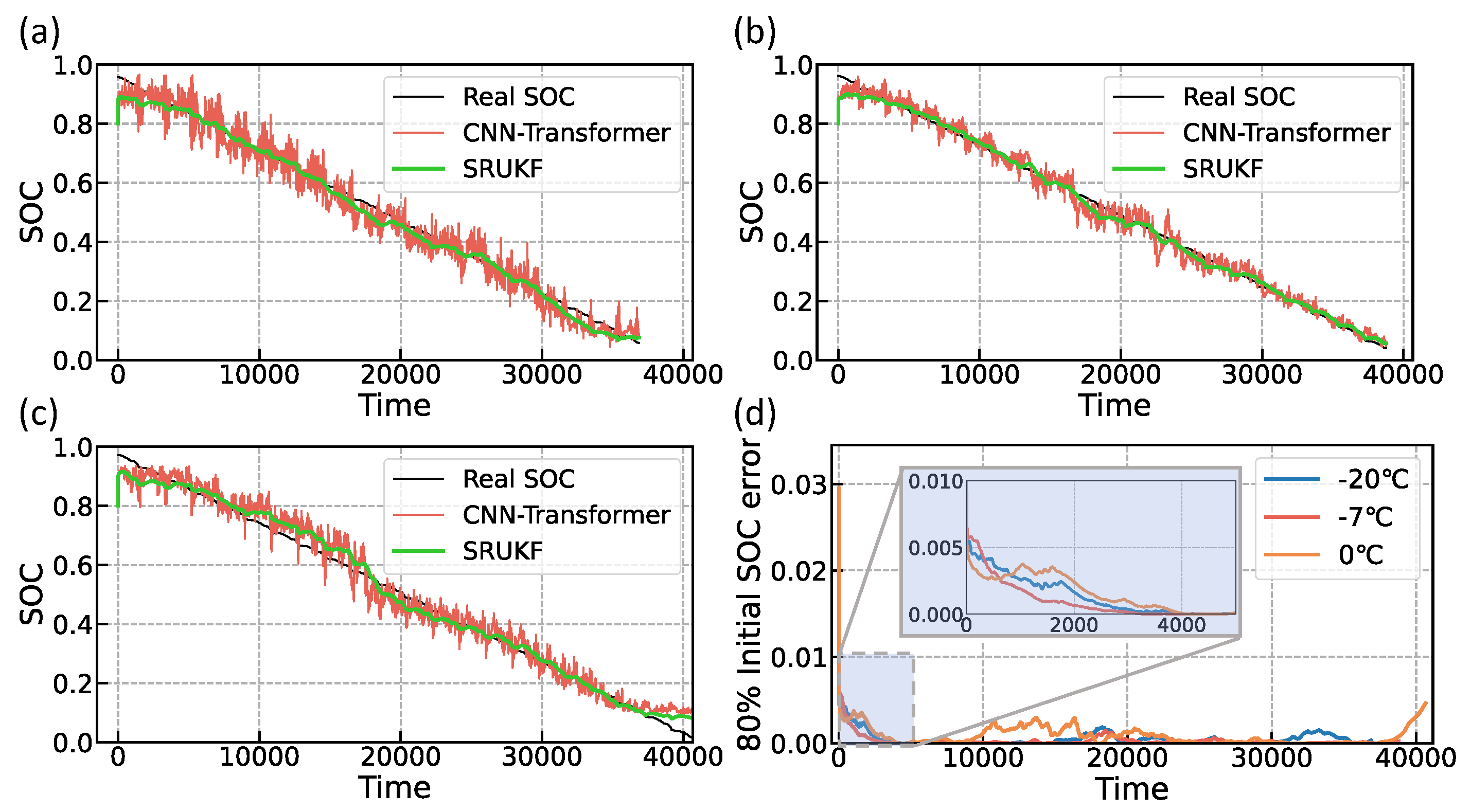
In order to verify the robustness of the SOC estimation method proposed in this paper, in this subsection, experiments are conducted by setting the initial SOC error of the SRUKF at different temperatures. The true initial SOC is 100%. The experimental results for 80% and 60% initial SOC are shown in Figure 11 and Figure 12, respectively. The experimental results at −20 °C, −7 °C, and 0 °C with 80% initial SOC are shown in Figure 11a–c, where the black line is the true SOC, the red line is the estimated SOC of the CNN-Transformer, and the green line is the estimated SOC of the SRUKF. As shown by the green line in Figure 11, the initial value of the SRUKF is set to 80%, which can quickly track the estimated value of the CNN-Transformer within 20 s. Due to the short time, the curve during this period is approximately vertical. Figure 11d shows the estimation error of 80% initial SOC at −20 °C, −7 °C, and 0 °C. As seen from the zoomed-in graph, the error can be converged to 1 × 10⁻³ within 4000 s. After 4000 s, although the error value has a large fluctuation, it can be stabilized to within 0.002. The fluctuation is caused by the local deviation of the neural network estimation from the real value. 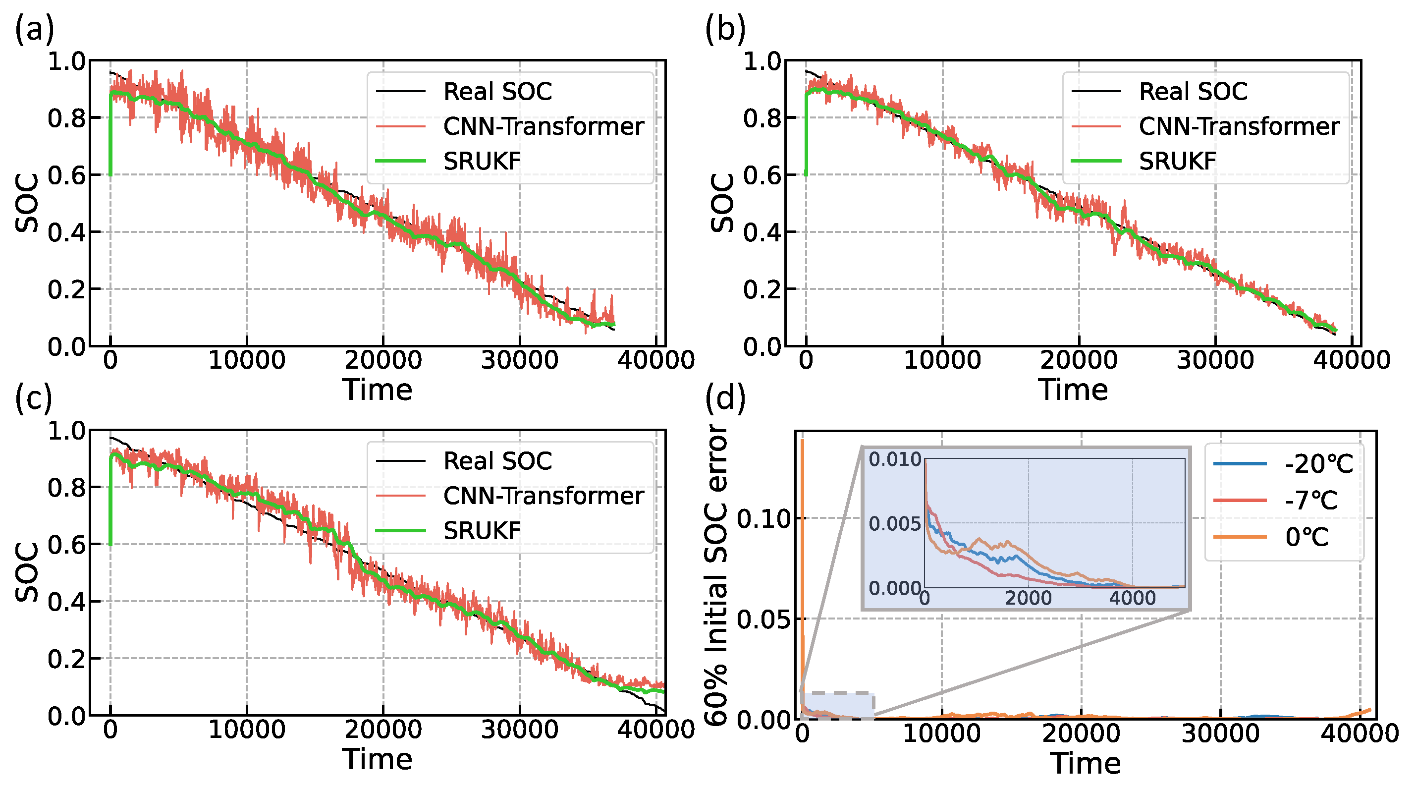Shown in Figure 12a–c are the experimental results of −20 °C, −7 °C, and 0 °C under 0.6 initial SOC, respectively. Similar to the estimation results under 0.8 initial SOC which was shown in Figure 11a–c, the SRUKF can track up the estimation value of the CNN-Transformer in a very short time. As depicted in Figure 12d, when starting with a 60% initial SOC, the error also converges to 0.001 within 4000 s. This is in contrast to the experimental results at 80% initial SOC, where the convergence trend for 60% initial SOC is sharper. It can be seen that the model has the ability to quickly adjust the estimation results, which is achieved by using the results of the neural network to update the state of the Coulomb counting method.

4.5. Comparison with Other Neural Networks

In this section, the estimation performance of the CNN-Transformer method proposed in this paper is compared with other popular machine learning techniques, such as LSTM and GRU, all of which are deep learning models designed for sequence data processing. Both LSTM and GRU are specialized forms of RNNs that overcome the issues of vanishing or exploding gradients found in traditional RNNs by incorporating a gating mechanism. In contrast, the Transformer discards the recurrent structure of RNNs altogether and uses self-attention and multi-head attention mechanisms to capture long-range dependencies in sequences, significantly enhancing the model’s performance. Although LSTM and GRU excel with certain sequence data types, the Transformer typically outperforms them when handling extremely long sequences. To ensure a fair comparison, the data processing and training procedures for the different networks were kept identical, with only the network architecture being altered.

Figure 13 and Figure 14, respectively, illustrate the prediction results of the LSTM and GRU models. In Figure 13a,c, we observe substantial deviations from the actual values at the tail of the −20 °C experiment and the middle of the 0 °C experiment, suggesting that the LSTM network lacks the robustness required for handling long-term sequential problems such as SOC estimation when compared to the Transformer network. 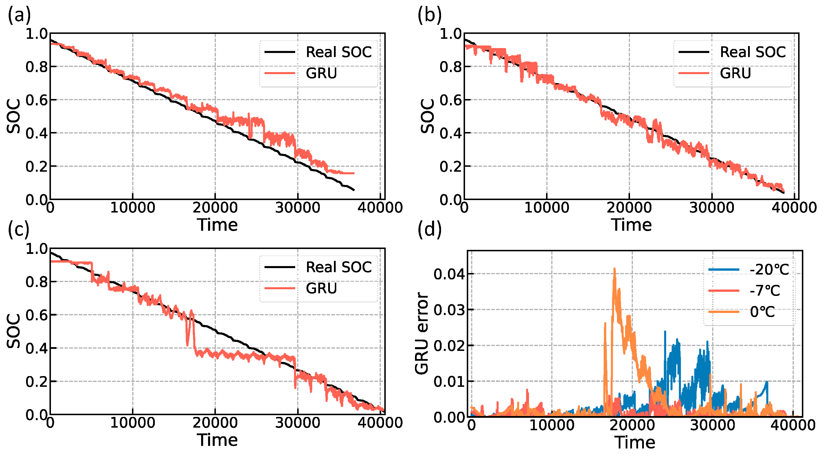Figure 13b, however, indicates a superior performance at −7 °C, which can be attributed to the higher data quality at that temperature. As illustrated in Figure 14a–c, the GRU network’s predictions share similarities with the LSTM network in terms of substantial local errors. The comprehensive RMSE and MAE are detailed in

Table 7. RMSE and MAE values of LSTM and GRU at −20 °C, −7 °C and 0 °C.

Temperature (°C)	RMSE (%)			MAE (%)
	CNN- Transformer	LSTM	GRU	CNN- Transformer	LSTM	GRU
−20	0.037327727	0.057181204	0.054153222	0.030301876	0.046788597	0.04215059
−7	0.026943953	0.028265816	0.026662869	0.020873434	0.021064911	0.021109136
0	0.042164227	0.051760989	0.059044589	0.03412065	0.035296289	0.040453324

, where the transformer network outperforms both the LSTM and GRU networks by delivering improvements of approximately 4.68% to 34.72% in terms of RMSE.

5. Conclusions

In the task of SOC estimation, the Coulomb counting method is heavily dependent on the accuracy of current measurements, model-based approaches hinge on parameter identification and frequently lack precision, and data-driven methods are plagued by poor interpretability and excessive sensitivity to data, resulting in estimation outcomes filled with noise. To tackle these challenges, this paper presents a new SOC estimation technique for lithium-ion batteries that merges the CNN-Transformer with SRUKF. Moreover, by harnessing ensemble learning theory, the proposed method accomplishes SOC estimation across a range of temperature conditions for batteries. Given the difficulties associated with low temperatures, such as reduced cell electrochemical reaction rates and an unstable voltage response, this study focuses on SOC estimation in cold environments. The primary contributions of this paper are encapsulated in three key areas:

(1)

Developing a CNN-Transformer network specifically for battery SOC estimation; it has shown robust predictive performance across datasets at −20 °C, −7 °C, and 0 °C.

(2)

By integrating SRUKF with CNN-Transformer networks for SOC estimation, this approach addresses the issue of noise in neural network SOC estimates and compensates for the cumulative drift error and the high dependence on current measurement accuracy that is inherent in Coulomb counting.

(3)

By applying ensemble learning theory, we have improved overall estimation performance through the combination of predictions from multiple models, enabling SOC estimation under any low-temperature scenario. This method allows the model to more effectively navigate the complex and variable conditions of real-world applications.

The specific content of the article is as follows: Initially, the CNN-Transformer benchmark model is trained and validated at three distinct temperature points (−20 °C, −7 °C, and 0 °C) to ascertain the precision and generalization capabilities of the proposed network. Subsequently, to validate the effectiveness of integrating SRUKF with neural networks, a comparison is conducted between the results of the CNN-Transformer network with SRUKF and one without any filtering. Following this, to evaluate the utility of ensemble learning, the concept of cross-validation is employed, where a set of V, I, and T data from one temperature point is used for prediction by models trained at the other two temperature points. The prediction outcomes are then linearly combined to derive the final predictive values. To test the robustness of the SOC estimation algorithm proposed in this paper, experiments are conducted with SRUKF initial SOC errors set at different temperatures. Specifically, with the true initial SOC at 100%, the initial SRUKF estimates are set to 80% and 60% for the experiments. Finally, the proposed network is compared with other neural networks, including LSTM and GRU networks, to demonstrate its advantages. The experimental results show that the SOC estimation method proposed in this study maintains a stable root mean square error between 2.69% and 4.22%. The introduction of SRUKF has improved the accuracy by 30.31% to 40.61% compared to the base model. Additionally, the method has exhibited high prediction accuracy in both ensemble learning and robustness validation experiments. The estimation precision of the proposed CNN-Transformer network at the three temperature nodes significantly surpasses that of the LSTM and GRU networks.

In future research, experiments at room temperature and high temperatures will be conducted to cover the full range of temperature scenarios for SOC estimation. Additionally, the influence of battery aging on SOC estimation will be explored, with the aim of enhancing estimation accuracy by jointly estimating SOC and SOH. Furthermore, the method proposed in this paper can be deployed in a vehicle-cloud collaborative framework, where model training is conducted in the cloud, and predictions are made on the vehicle side.