Abstract
This paper presents three approaches to estimating the battery parameters of the electrical equivalent circuit model (ECM) based on electrochemical impedance spectroscopy (EIS); these approaches are referred to as (a) least squares (LS), (b) exhaustive search (ES), and (c) nonlinear least squares (NLS). The ES approach is assisted by the LS method for the rough determination of the lower and upper bound of the ECM parameters, and the NLS approach is incorporated with the Monte Carlo run such that different initial guesses can be assigned to improve the goodness of EIS fitting. The proposed approaches are validated using both simulated and real EIS data. Compared to the LS approach, the ES and NLS approaches show better fitting accuracy at various noise levels, whereas in both the validation using simulated EIS data and actual EIS data collected from LG 18650 and Molicel 21700 batteries, the NLS approach shows better fitting accuracy than that of LS and ES approaches. In all cases, compared with the ES approach, the computational time of the NLS approach is significantly faster, and compared with the LS approach, the NLS approach shows a minimal difference in computational time and considerably better fitting performance.
1. Introduction
EIS has been used to study the ion transport properties and electrode/electrolyte interfacial behavior of Li-ion batteries, providing insights into their performance and potential avenues for improvement [1]. In a typical EIS experiment, a small-amplitude sinusoidal current/voltage signal is applied to the battery, and the resulting voltage/current response is measured over a range of frequencies [2]. The resulting impedance data can be analyzed using equivalent electrical circuit models to extract information on the underlying electrochemical behavior [3]. EIS can provide detailed information on the electrochemical processes occurring within the battery, including the charge transfer kinetics, ion transport properties, and electrode/electrolyte interfacial behavior [4]. Pastor-Fernández et al. [5] conducted battery aging identification and quantification research by analyzing the EIS of four parallel Li-ion cells.
The EIS can be characterized using an equivalent circuit model (ECM), which represents the battery as a combination of resistive, inductive, and capacitive components; then, the ECM parameters can be identified by fitting the ECM to the measured EIS data [6]. There are different ECM models relevant to different types of batteries. This requires prior knowledge of battery chemistry [7]; furthermore, by iteratively adjusting the ECM parameters, the best fit can be obtained.
There are various approaches to fit the ECM model to the measured EIS data. For instance, the nonlinear least squares (NLS) approach can be used to estimate the parameters of a nonlinear model; this aims to optimize the nonlinear function such that the difference between experimental data and the estimations based on the ECM model can be minimized [8]. Boukamp [9] applied a Nonlinear Least Squares Fit (NLLSF) approach to analyze the electrochemical impedance data with the ECM model; in this research, it also mentioned that the selection of starting point is critical for the fit procedure.
Furthermore, Genetic Algorithm (GA) is a population-based optimization approach that can also be used in fitting the ECM to EIS data; however, the computational complexity of this approach will increase significantly with the number of ECM parameters, which means that a large number of iterations are needed. Furthermore, the selection of population size, mutation rate, and crossover rate requires continuous tuning to reach the optimal estimation [10].
The complex nonlinear least squares (CNLS) approach is widely used to fit the ECM model to EIS data. Pastor-Fernández et al. [5] applied the CNLS algorithm to fit ECM to the EIS data measured from four Li-ion batteries. Feng et al. [11] applied the CNLS approach to estimate ECM parameters using the EIS data collected from a battery cell at different SOC levels and temperatures. The drawback of this approach is that the fitting accuracy can easily be affected by the initial guess of the ECM parameters; for instance, the optimization algorithm may converge to a local minimum instead of converging to a global minimum if the initial guess is selected inappropriately; this will lead to inaccurate ECM parameter estimation. Also, the CNLS approach requires the specification of ECM models, such as the number of components and the arrangement of RC circuits, which leads to extra work being carried out before the fitting process. Furthermore, CNLS is a computationally expensive approach, and it also requires an appropriate selection of initial conditions to obtain accurate fitting [12].
Ghadi [13] applied the least squares (LS) approach to fit the EIS data to identify ECM parameters by assuming the solid electrolyte interphase (SEI) arc and charge transfer (CT) arc to be semicircles, and that the solid electrolyte interphase resistance and charge transfer resistance are the diameters of the SEI arc and the CT arc, respectively. The merit of this approach is that the estimation of the parameters can be expressed in closed form; however, the main drawback is that the accuracy of this approach is not sufficient. One improvement is to apply the exhaustive search (ES) approach to identify more accurate estimations of ECM parameters with the assistance of the LS approach; in this paper, the ES approach will be explained in detail.
Furthermore, we proposed a novel NLS approach which only needs to define the objective function; then, it randomly chooses the initial guess in each Monte Carlo Run and the estimated parameters that can reach the lowest fitting error are selected. While the ES approach can somewhat reach a better fitting accuracy compared with the LS approach, the computational time is still very slow. Furthermore, the computational time of the NLS approach is much faster than that of the ES approach; in addition, compared to the LS and ES approaches, NLS shows higher fitting accuracy.
The contributions of this paper can be summarized as follows:
- This paper compares the performance of the LS, ES, and Monte Carlo-based NLS approaches to identify battery ECM parameters.
- Compared to the LS approach presented in [13], the ES and the NLS approaches can significantly boost the fitting accuracy of EIS measurements.
- This paper presents a novel approach to implementing NLS through Monte Carlo runs. At each Monte Carlo run, the initial parameters required for the NLS approach are selected randomly. This approach results in better accuracy and a much faster computation time than the ES approach.
- All the methods are validated using both simulated EIS data with different noise levels and real EIS data collected from two different types of Li-ion batteries; the fitting performance of the NLS approach outweighs other approaches in all cases.
The remainder of the paper is organized as follows: Section 2 describes the analysis of battery ECM parameters via EIS in the frequency domain. Section 3 describes the algorithms to estimate ECM parameters using the least squares approach. Section 4 describes algorithms of exhaustive search and the Monte Carlo-based nonlinear least squares approach is explained in Section 5. The implementation procedure is explained in Section 6. Results are discussed in Section 7. Section 8 concludes the paper.
2. Analysis of ECM Parameters in Frequency Domain
EIS is a widely used technique to investigate the impedance response of the battery. To measure the EIS, a small perturbation current with a wide range of frequencies (0.01 Hz to 10 kHz) is injected into the battery; then, by using the discrete Fourier transform (DFT), the measured voltage and current in the time domain can be converted to the frequency domain. Thus, the impedance in the frequency domain can be analyzed [14,15]. The battery EIS can then be represented by the real and imaginary part of the impedance on the complex plane to form the Nyquist plot [16,17]. This plot represents the impedance spectrum of the battery at a range of frequencies; the ECM parameters can be estimated by fitting the EIS data with suitable fitting algorithms [13,18].
As shown in Figure 1, the 2-RC Adaptive Randles (AR) ECM is selected to fit the EIS that shows a diffusion arc in low frequencies and SEI/CT arc in medium frequencies; in this model, the Warburg element is placed in series with instead of being placed as an independent element. This is due to the consideration of mass transport phenomenon in battery cells’ electrochemical reactions [19]. The AR-ECM consists of the following components [15]:
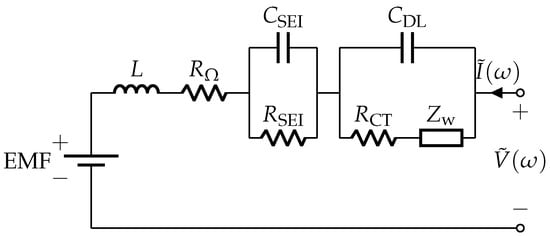
Figure 1.
Adaptive Randles equivalent circuit model (AR-ECM) of a battery.
- Voltage source, ;
- Stray inductance, L;
- Ohmic resistance, ;
- Solid electrolytic interface (SEI) resistance, ;
- SEI capacitance, ;
- Charge transfer (CT) resistance, ;
- Double-layer (DL) capacitance, ;
- Warburg impedance, .
Figure 2 shows the Nyquist plot relevant to the AR-ECM. According to this figure, the AC impedance corresponding to the AR-ECM can be written as [13]
where denotes the impedance in the RL arc, denotes the impedance in the SEI arc, and denotes the impedance in the CT arc and DF arc.
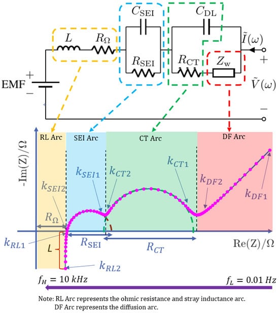
Figure 2.
The theoretical Nyquist plot corresponding to the AR-ECM.
3. Least Squares Approach
To solve the problem of ECM parameter estimation, Ghadi [13] applied the LS algorithm to fit the EIS measurements; furthermore, this approach can express the estimation of ECM parameters in closed form. In this section, an improved LS approach to AR-ECM parameter estimation is presented.
Figure 2 shows the impedance spectrum/Nyquist plot corresponding to the AR-ECM shown in Figure 1. Each data point in the Nyquist plot is obtained through the procedure as shown in Figure 3, where and are the measured voltage and current in the time domain while injecting sinusoidal current to the battery at different frequencies; and are the Fourier transform of the corresponding voltage and current measurements; and the real part and imaginary part of the measured impedance can be defined as follows:
where .
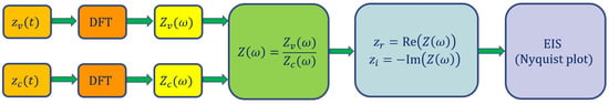
Figure 3.
The procedure to obtain battery EIS [20].
It can be observed that the Nyquist plot needs to be divided into four parts to see how it is directly related to the AR-ECM. The feature points of the Nyquist plot are indicated by index and in the DF arc; are indicated by and in the CT arc; are indicated by and in the SEI arc; and are indicated by and in the RL arc. Different parts of the Nyquist plot represent the battery’s impedance at different frequencies [18]. In this paper, to keep the consistency of nomenclature, we define the following:
- is the index of the first data point in the DF arc; in this paper, we define .
- is selected such that the data points from to follow the linear line.
- is selected at the beginning of the CT arc such that the data points start to follow the arc.
- is selected at the end of the CT arc such that data points between follow the CT arc.
- Similarly, is selected at the beginning of the SEI arc.
- is selected at the end of the SEI arc such that data points between follow the SEI arc.
- is selected at the beginning of the RL arc.
- is selected at the end of the RL arc.
3.1. Estimation of Ohmic Resistance and Stray Inductance
As shown in Figure 2, based on the impedance measurements in the RL arc, the estimation of ohmic resistance can be estimated as follows [13,18]:
and stray inductance L can be estimated using the improved method:
3.2. Estimation of Diffusion Arc’s Gradient m
Considering the imaginary part of the measured impedance and the real part of the measured impedance in the Diffusion arc, it can be represented with a linear model [21]:
Assuming the measurements are from to , as shown in Figure 2, the following can be written as follows [13,18]:
Equation (6) can be written in the matrix form:
m and a can be estimated using the LS approach:
Algorithm 1 estimates quantities (list) based on the following impedance values:
In this paper, the uppermost bound of the DF arc is denoted as , the lowest bound of the CT arc is denoted as , and the lowest bound of the SEI arc is denoted as ; these boundaries can be identified by applying a moving average filter (MAF) to process the measured impedance data via Algorithm 1, where every 10 data points are selected for calculating the smoothed value. The filtered EIS data are shown in Figure 4a. The algorithms presented in this paper are written utilizing MATLAB 2020a syntax. Algorithm 1 uses the following MATLAB commands: smooth, length, find, min, break, continue.
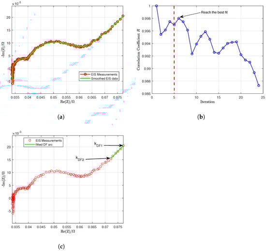
Figure 4.
DF arc fitting process. (a) Smooth the EIS using MAF. (b) Find the highest correlation coefficient r when fitting the DF arc. (c) Fitted DF arc.
| Algorithm 1 Boundary identification. |
| Input: , . |
| Output: , , |
|
The gradient m of the diffusion arc can be estimated by fitting the diffusion arc with the linear model mentioned in (5) and searching for the best fit using Algorithm 2. The fitting process is also demonstrated in Figure 4b,c. Algorithm 2 uses the following MATLAB commands: mean, find, max.
| Algorithm 2 Diffusion arc fitting. | |
| Input: , , | |
| Output: , | |
| 1: for do | |
| 2: , | |
| 3: , | |
| 4: Estimate gradient in iteration via Equations (5)–(9) | |
| 5: Estimate imaginary part of the impedance based on the fitted linear model. | |
| 6: | ▹ the sum of error squares |
| 7: | ▹ the total sum of squares around the mean |
| 8: | ▹ correlation coefficient |
| 9: end for | |
| 10: | ▹ written in MATLAB syntax; the first four data points are avoided due to possible anomalies. |
| 11: | |
3.3. First Estimation of Warburg Coefficient
From the observation of EIS measurements in [18], it was found that the gradient of the diffusion arc varies with the SOC level; in addition, gradients may be different even at the same SOC level of batteries from two different manufacturers. Therefore, an improved method to represent Warburg impedance is defined mathematically as
where is the Warburg coefficient, m is the gradient of the fitted DF arc, and j is .
It must be emphasized here that, in [13], the gradient was assumed to be . In this paper, we propose estimating the gradient m to achieve better EIS fitting.
It can be shown, based on (1), that the Warburg impedance is significant only at lower frequencies. In Figure 2, impedance measurements from to are selected to estimate the Warburg coefficient (we define , and is obtained via Algorithm 2). Considering the real part of the impedance in the diffusion arc [13,18]
where .
3.4. Estimation of and
As shown in Figure 2, to fit the SEI arc precisely, we select feature points that lie between and . Let us denote the impedance measurements in the SEI arc as
The estimation of is to fit the SEI arc using a semicircle with its centre lying on the real axis; the coordinate of this semicircle’s centre can be denoted as (, 0); the radius of the semicircle can be denoted as ; and, thus, the measurements in (16) should satisfy the equation of the semicircle [18]:
Let and , thus
And (18) can be rewritten as
In the matrix form, (21) can be written as
Using the LS algorithm, the estimate of will be given by
The estimates of c and d are as follows:
From Figure 2, is the diameter of the SEI arc; thus, by substituting the values of c and d in (20), the estimate of is
The estimated centre of the semicircle can then be expressed as
The fitting accuracy of the SEI arc can be evaluated as [22]
where is the geometrical distance between the actual EIS data point and predicted EIS data point, which is defined as
It can be shown in (1) that when the frequency is very high, the impedance in the CT arc and diffusion arc will be minimal so that it is negligible; thus, we assume the term will be zero, that is
Therefore, the impedance in the SEI arc can be expressed as follows [18]:
Take the imaginary part on both sides of the above equation,
Finally, average all the estimates to obtain the final estimate:
The use of the LS approach to identify and via the automatic selection of feature points is fully described in Algorithm 3. In addition, Figure 5a shows the RMSE of the fitted SEI arc in each iteration and Figure 5b shows the SEI arc, which is selected since it can reach the best fit. Algorithm 3 uses the following MATLAB commands: floor, find, length.
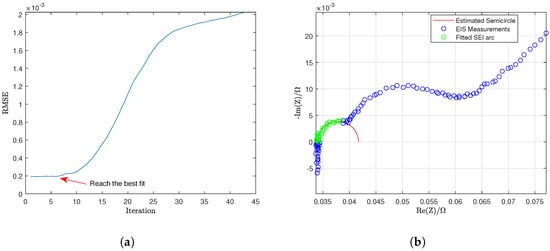
Figure 5.
Fitted SEI arc using LS approach. (a) RMSE of the fitted SEI arc. (b) Best fitting of SEI arc.
| Algorithm 3 Estimate and via automatic feature detection. |
| Input: , , , , |
| Output: , . |
|
3.5. Estimation of and
It can be observed in Figure 2 that to fit the CT arc using a semicircle precisely, we need to select feature points that lie between to ; therefore, the impedance measurements in the CT arc can be denoted as follows:
Assuming that the centre of the semicircle lies on the real axis, which is noted as (, 0), the radius of the semicircle can be noted as ; thus, the measurements in (39) should satisfy the equation of the semicircle [18]:
Let and , thus
And (41) can be rewritten as
In the matrix form, (44) can be written as
From (45), can be estimated using the LS algorithm
Thus, the estimates of a and b are as follows:
As shown in Figure 2, is the diameter of the CT arc; thus, by substituting the values of a and b in (43), the estimate of is
The estimated centre of the semicircle can then be expressed as
The fitting accuracy of the CT arc can be evaluated as [22]
where is the geometrical distance between the actual EIS data point and predicted EIS data point, which is defined as [22]
Based on (1),
Therefore, the impedance in the CT arc and DF arc can be expressed as follows:
Taking the imaginary part on both sides of (56), and substituting with the expression given in (13), we obtain
Substituting L, , , , and with the estimations given in (4), (3), (25), (38), (48) and (15), respectively, in the above equation at
Finally, average all the estimates to obtain the final estimate:
The use of the LS approach to identify and via the automatic selection of feature points is shown in Algorithm 4. Furthermore, Figure 6a shows the RMSE of the fitted CT arc in each iteration, and Figure 6b shows the CT arc selected since it can reach the best fit. Algorithm 4 uses the following MATLAB commands: floor, round.
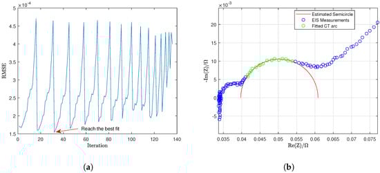
Figure 6.
Fitted CT arc using LS approach. (a) RMSE of the fitted CT arc. (b) Best fitting of CT arc.
| Algorithm 4 Estimate and via automatic feature detection. |
| Input: , , , , , , , , , |
| Output: , , |
|
3.6. Evaluation of the General Fitting Accuracy
In the complex plane, the absolute value of the error between the measured EIS and estimated EIS is actually the distance between measured EIS data points and estimated EIS data points, as shown in Figure 7, , where , … are the distances between the measured EIS data point and estimated EIS data point , which can be used to evaluate the fitting accuracy. The distance is represented as follows:
where n is the number of measurements, .
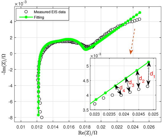
Figure 7.
Geometrical distance between measured EIS data point and predicted EIS data point.
Therefore, the evaluation of EIS fitting can be expressed as
where is the measured impedance at ; is the impedance estimation at , which is computed based on (1) with the estimated ECM parameters; N is the total number of measurements; and denotes the absolute value of the complex number.
The goal is to fit the EIS measurements such that the fitted EIS can achieve the lowest MAE.
The percentage error of the estimated parameters can be expressed as follows:
4. Exhaustive Search Approach
The Exhaustive Search (ES) approach aims to improve the goodness of fitting by searching the optimal value of each parameter based on the initial estimations of two RC components and gradient m identified via the LS approach; this process is shown in Figure 8.
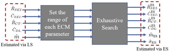
Figure 8.
The principle of the ES approach.
4.1. Second Estimation of Warburg Coefficient
Assume , L, , , , and m are given, based on (54),
thus,
then,
then, the Warburg impedance can also be expressed as:
Take the real part on both sides of the above equation, at ,
The real part of the Warburg impedance can be noted as follows:
Taking the real part on both sides of (12), we obtain
Thus,
Finally, average all the estimates to obtain the final estimate:
4.2. Specify the Range of Parameters for Exhaustive Search
As presented in Section 3, the rough estimations of ECM parameters are given; therefore, we can assign the lower and upper bound for each parameter such that the exhaustive search approach can identify the most suitable parameter between the boundary. As shown in Algorithm 5, the range of each ECM parameter is assigned based on the empirical coefficient. In this paper, the size of possible values in each ECM parameter is restricted to 20, such that the computational time is within the acceptable range. Algorithm 5 uses the MATLAB command: linspace.
| Algorithm 5 Set the range of ECM parameters estimated by the LS approach. |
| Input: , , , , |
| Output: , , , , |
|
4.3. Implement Exhaustive Search
Algorithm 6 describes the ES approach that can be applied to precisely identify the ECM parameters, where the input is estimated via (3) and is estimated via (4). Figure 9 shows the MAE evaluated from the initial iteration throughout the end of the exhaustive search process; by finding the lowest MAE in this figure, one can identify the best estimation of ECM parameters via the ES approach.
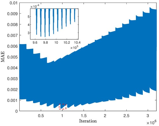
Figure 9.
Find the lowest MAE of the ES approach .
| Algorithm 6 Exhaustive search approach. |
| Input: , , , , , , |
| Output: , |
|
5. Nonlinear Least Squares Approach
The concept of implementing the NLS approach based on the Monte Carlo run is shown in Figure 10. This approach randomly selects initial guesses of the ECM parameters in each Monte Carlo run to fit the EIS data in different cases.
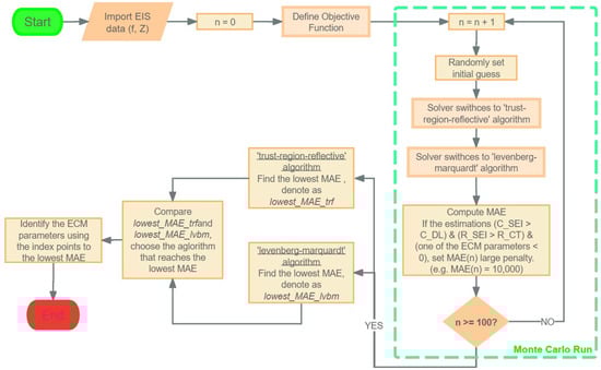
Figure 10.
Monte Carlo-based nonlinear least squares approach.
5.1. Objective Function
The goal is to find the optimized ECM parameters to minimize the following function:
where,
and is the measured impedance at , N is total number of measurements, and denotes the absolute value of the complex number.
The nonlinear least squares approach is implemented in MATLAB using the built-in function to fit the EIS data.
5.2. Initial Guess
Instead of setting the lower bound and upper bound for the NLS approach, in this paper, we randomly select an initial guess in each Monte Carlo run to try different NLS fittings based on different initial guesses. In this way, one can find the best fit among all cases. In MATLAB the initial guess is defined as follows:
5.3. Algorithm Switch
To reach the best fit, the NLS approach will apply a ‘trust-region-reflective’ algorithm [23,24] and the ‘Levenberg–Marquardt’ algorithm [25,26,27] to fit the EIS data with different initial guesses. After that, the algorithm that can achieve the lowest mean absolute error (MAE) will be selected as the approach that can reach the best fit. The detailed approach is shown in Algorithm 7. This algorithm uses the following MATLAB commands: ‘abs’ and ‘randn’.
| Algorithm 7 NLS approach. | |
| Input: measured impedance | |
| Output: , | |
| 1: Define objective function | |
| 2: | |
| 3: while n ≤ 100 do | |
| 4: | ▹ Randomly set initial guess |
| 5: Solver switches to ‘trust-region-reflected’ algorithm | |
| 6: Solver switches to ‘levenberg-marquardt’ algorithm | |
| 7: Compute MAE | |
| 8: | |
| 9: end while | |
| 10: Find the lowest MAE computed by ‘trust-region-reflective’ algorithm, denote as | |
| 11: Find the lowest MAE computed by ‘levenberg-marquardt’ algorithm, denote as | |
| 12: if then | |
| 13: | |
| 14: else | |
| 15: | |
| 16: end if | |
| 17: ← Identify the ECM parameters using the index points to the lowest MAE | |
| 18: Compute Percentage Error (In EIS simulation data validation procedure) | |
6. Implementation
This paper implements three ECM parameter estimation approaches in MATLAB R2020a with a 3 GHz Processor and 16 GB RAM.
6.1. Simulate EIS Data
The simulated EIS data were generated using Algorithm 8, where the frequency ranges from 0.01 Hz to 10 kHz, and the number of EIS measurements is 121; this is to keep conformity with the sampling size we set in the EIS experiment [18]. In addition, Table 1 shows the true ECM parameters for simulating EIS data. To generate various noise levels for the simulated EIS measurements, we implement Gaussian noise with zero-mean, standard deviation , and independent outcome.

Table 1.
True ECM parameters used for EIS simulation.
Algorithm 8 uses the MATLAB commands: ‘linspace’, ‘real’, ‘imag’, and ‘randn’.
| Algorithm 8 EIS simulation. | |
| Input: , , n | |
| : True ECM paramters, vector | |
| Output: , , : Frequencies ranges from the lowest to the highest | |
| 1: | |
| 2: , | |
| 3: | |
| 4: | ▹ Angular frequency, vector |
| 5: Compute impedance via Equation (1) based on the given ECM parameters | ▹ Where, |
| 6: ← + * | |
| 7: ←+ * | |
6.2. Collect Real EIS Data
The impedance data are measured from two Li-ion batteries: LG 18650 and Molicel 21700. In addition, the specifications of LG and Molicel batteries are shown in ([18], Table 1). The data were collected using the Arbin battery cycler (Model: LBT21084UC), which has 16 channels that can operate in parallel. In this experiment, eight channels were used to collect data simultaneously at room temperature (23 °C).
The EIS data were measured by the EIS device (Gamry Interface 5000P, Gamry Instruments, Inc., Warminster, PA, USA). We operated the Gamry EIS device and Arbin battery cycler using the software MITS Pro 8.0 provided by Arbin Instruments (College Station, TX, USA). The voltage measurement error of the Gamry EIS device is 0.2 mV, as specified from [28]. In this paper, we validated LS, ES, and NLS approaches on EIS data collected from one LG and one Molicel battery when the SOC was at 90%, 50% and 10%, while discharging from a fully charged state.
7. Results
In this section, fitting results obtained from the simulated and real EIS data are shown and discussed.
7.1. Estimation Results of ECM Parameters Using Simulated EIS Data
The comparisons of simulated EIS data fitted by the LS, ES, and NLS approaches are shown in Figure 11a–d. It can be observed that the LS approach shows insufficient goodness of fitting, whereas the ES and NLS approaches generally reach considerable fitting accuracy. Table 2 shows that at any noise level, the computational time of the LS approach is the fastest; however, the fitting accuracy MAE is the lowest. On the contrary, the ES approach has the slowest computational time, but the fitting accuracy is significantly improved compared with the LS approach. The NLS approach reaches the lowest MAE and is considerably faster than the ES approach. Furthermore, with the noise level decreasing, the MAE decreases.
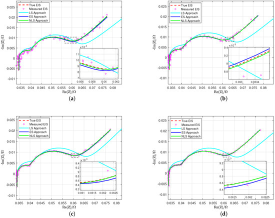
Figure 11.
Fitting simulated EIS measurements via LS, ES, and NLS approaches at different noise levels. (a) = 0.6046 . (b) = 0.3400 . (c) = 0.1912 . (d) = 0.1075 .
Table 2.
Esitmated ECM parameters, computational time, and accuracy of using LS, ES and NLS approaches to fit simulated EIS data.
As shown in Figure 12a–d, it is clear that at any noise level, the percentage error of the estimated RC components reaches the highest when using the LS approach and reaches the lowest when using NLS approach, except for that the percentage error of estimated via NLS is higher than that estimated via ES when = 0.1075 . In addition, at any noise level, the percentage errors of estimated ECM parameters using the NLS approach are well below 5%; this shows significantly higher estimation accuracy compared with the ES and LS approaches.
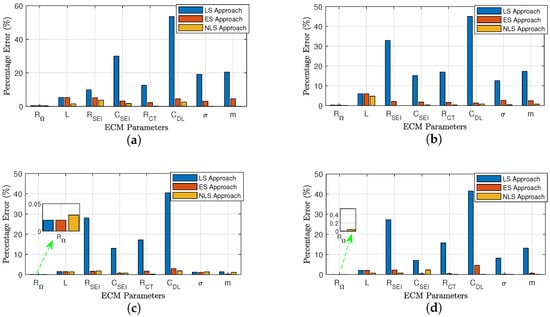
Figure 12.
Percentage difference between true and estimated ECM parameters at different noise levels. (a) = 0.6046 . (b) = 0.3400 . (c) = 0.1912 . (d) = 0.1075 .
7.2. Estimation Results of ECM Parameters Using Real EIS Data
LG 18650 and Molicel 21700 Li-ion batteries were selected to validate whether the LS, ES, and NLS approaches show consistency in fitting real EIS data that are collected at , , and SOC.
Figure 13a–c show the fitted EIS of LG 18650 battery using LS, ES, and NLS approaches; Figure 13d–f show the fitted EIS of Molicel battery using the same approaches. Compared to the LS approach, both the ES and NLS approaches show higher fitting accuracy.
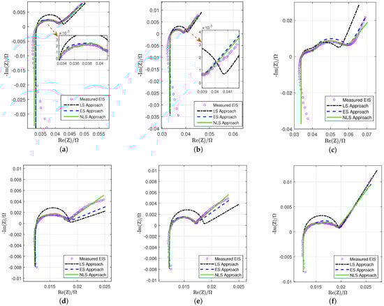
Figure 13.
Fitting real EIS measurements of LG and Molicel batteries at different SOC levels via LS, ES, and NLS approaches. (a) LG battery at 90% SOC. (b) LG battery at 50% SOC. (c) LG battery at 10% SOC. (d) Molicel battery at 90% SOC. (e) Molicel battery at 50% SOC. (f) Molicel battery at 10% SOC.
In Table 3, it can be observed that when fitting the LG battery’s EIS data at any SOC level, the EIS approach outperforms the ES and LS approaches; furthermore, in terms of the computational time, the ES approach is considerably slower than the NLS approach. Though the LS approach is the fastest, the MAE is the highest among all SOC levels. Additionally, in Table 4, the validation on the Molicel battery shows consistent results.
Table 3.
Estimated ECM parameters, computational time, and accuracy of using LS, ES and NLS approaches to fit real EIS data collected from LG 18650 battery while discharging.
Table 4.
Estimated ECM parameters, computational time, and accuracy of using LS, ES and NLS approaches to fit real EIS data collected from Molicel 21700 battery while discharging.
8. Conclusions and Discussions
This paper presented the LS, ES, and NLS approaches to extract ECM parameters through battery impedance measurements. Compared to the LS approach, the ES and NLS approach can extract ECM parameters more accurately. Though the LS approach shows insufficient goodness of fitting at various noise levels, it can boost the fitting accuracy of the ES approach by offering initial estimations; however, it is worth mentioning that while the ECM contains more than two RC components, the computation time will increase significantly such that this approach will be infeasible.
When fitting the simulated EIS data, both the ES and NLS approaches show considerably high accuracy at each noise level, and the fitting accuracy increases as the noise decreases. When fitting the battery EIS measurements, the NLS approach still shows faster and more accurate fitting performance than the ES approach; this result is validated in simulated EIS data.
In future works, we will investigate deploying the NLS approach to the BMS board combined with the rapid EIS measurement hardware to improve the accuracy and computational time for ECM parameters estimation; the BMS can then adopt these precisely estimated ECM parameters for more accurate online SOC/SOH estimation.
Author Contributions
Conceptualization, Y.W. and B.B.; methodology, Y.W.; software, Y.W.; validation, Y.W. and B.B.; formal analysis, Y.W.; investigation, Y.W.; resources, Y.W.; data curation, Y.W.; writing—original draft preparation, Y.W.; writing—review and editing, Y.W. and B.B.; visualization, Y.W.; supervision, B.B.; project administration, B.B.; funding acquisition, B.B. All authors have read and agreed to the published version of the manuscript.
Funding
This research received no external funding.
Data Availability Statement
The raw data supporting the conclusions of this article will be made available by the authors on request.
Acknowledgments
B. Balasingam would like to acknowledge the Natural Sciences and Engineering Research Council of Canada (NSERC) for the financial support under the Discovery Grants (DG) program (funding reference number RGPIN-2018-04557) and the Alliance Program (funding reference number ALLRP 561015).
Conflicts of Interest
The authors declare no conflict of interest.
References
- Ranque, P.; Gonzalo, E.; Armand, M.; Shanmukaraj, D. Performance-based materials evaluation for Li batteries through impedance spectroscopy: A critical review. Mater. Today Energy 2023, 34, 101283. [Google Scholar] [CrossRef]
- Islam, S.R.; Park, S.-Y. Precise online electrochemical impedance spectroscopy strategies for li-ion batteries. IEEE Trans. Ind. Appl. 2019, 56, 1661–1669. [Google Scholar] [CrossRef]
- Mandal, S.; Barai, P.; Mukherjee, P.; Sharma, R. An impedance-based study on the ageing of Li-ion batteries. Electrochim. Acta 2019, 307, 161–174. [Google Scholar]
- Ju, H.; Wu, J.; Xu, Y. Revisiting the electrochemical impedance behaviour of the LiFePO4/C cathode. J. Chem. Sci. 2013, 125, 687–693. [Google Scholar] [CrossRef]
- Pastor-Fernández, C.; Widanage, W.D.; Marco, J.; Gama-Valdez, M.-Á.; Chouchelamane, G.H. Identification and quantification of ageing mechanisms in lithium-ion batteries using the eis technique. In Proceedings of the 2016 IEEE Transportation Electrification Conference and Expo (ITEC), Dearborn, MI, USA, 27–29 June 2016. [Google Scholar]
- Meddings, N.; Heinrich, M.; Overney, F.; Lee, J.S.; Ruiz, V.; Napolitano, E.; Seitz, S.; Hinds, G.; Raccichini, R.; Gaberšček, M.; et al. Application of electrochemical impedance spectroscopy to commercial Li-ion cells: A review. J. Power Sources 2020, 480, 228742. [Google Scholar] [CrossRef]
- Theiler, M.; Schneider, D.; Endisch, C. Experimental Investigation of State and Parameter Estimation within Reconfigurable Battery Systems. J. Batteries 2023, 9, 145. [Google Scholar] [CrossRef]
- Tian, N.; Wang, Y.; Chen, J.; Fang, H. One-shot parameter identification of the Thevenin’s model for batteries: Methods and validation. J. Energy Storage 2020, 29, 101282. [Google Scholar] [CrossRef]
- Boukamp, B. A Nonlinear Least Squares Fit procedure for analysis of immittance data of electrochemical systems. Solid State Ion. 1986, 20, 31–44. [Google Scholar] [CrossRef]
- Li, X.; Chen, C.; Lü, X.; Zhang, W.; Liu, J.; Yu, H. A review on the applications of electrochemical impedance spectroscopy in batteries. J. Energy Chem. 2021, 53, 146–162. [Google Scholar]
- Feng, F.; Yang, R.; Meng, J.; Xie, Y.; Zhang, Z.; Chai, Y.; Mou, L. Electrochemical impedance characteristics at various conditions for commercial solid–liquid electrolyte lithium-ion batteries: Part. 2. Modeling and prediction. Energy 2022, 243, 123091. [Google Scholar] [CrossRef]
- Sihvo, J.; Roinila, T.; Stroe, D.-I. Novel Fitting Algorithm for Parametrization of Equivalent Circuit Model of Li-Ion Battery from Broadband Impedance Measurements. IEEE Trans. Ind. Electron. 2021, 68, 4916–4926. [Google Scholar] [CrossRef]
- Ghadi, M.A. Performance Analysis and Improvement of Electrochemical Impedance Spectroscopy for Online Estimation of Battery Parameters. Master’s Thesis, University of Windsor, Windsor, ON, Canada, 2021. [Google Scholar]
- Barsoukov, E.; Ross Macdonald, J. (Eds.) Impedance Spectroscopy: Theory, Experiment, and Applications, 3rd ed.; John Wiley & Sons: Nashville, TN, USA, 2018; ISBN 9781119074083. [Google Scholar]
- Orazem, M.E.; Tribollet, B. Electrochemical Impedance Spectroscopy; John Wiley & Sons, Inc.: Hoboken, NJ, USA, 2008; ISBN 9780470041406. [Google Scholar]
- Balasingam, B.; Pattipati, K.R. On the identification of electrical equivalent circuit models based on noisy measurements. IEEE Trans. Instrum. Meas. 2021, 70, 1–16. [Google Scholar] [CrossRef]
- Waag, W.; Käbitz, S.; Sauer, D.U. Experimental investigation of the lithium-ion battery impedance characteristic at various conditions and aging states and its influence on the application. Appl. Energy 2013, 102, 885–897. [Google Scholar] [CrossRef]
- Wu, Y.; Sundaresan, S.; Balasingam, B. Battery parameter analysis through electrochemical impedance spectroscopy at different state of charge levels. J. Low Power Electron. Appl. 2023, 13, 29. [Google Scholar] [CrossRef]
- Orazem, M.E.; Ulgut, B. On the proper use of a Warburg impedance. J. Electrochem. Soc. 2024, 171, 040526. [Google Scholar] [CrossRef]
- Lu, P.; Li, M.; Zhang, L.; Zhou, L. A novel fast-EIS measuring method and implementation for lithium-ion batteries. In Proceedings of the 2019 Prognostics and System Health Management Conference (PHM-Qingdao), Qingdao, China, 25–27 October 2019. [Google Scholar]
- Chatterjee, S.; Hadi, A.S. Regression Analysis by Example, 5th ed.; Wiley-Blackwell: Hoboken, NJ, USA, 2015. [Google Scholar]
- Baum, M.; Klumpp, V.; Hanebeck, U.D. A novel Bayesian method for fitting a circle to noisy points. In Proceedings of the 2010 13th International Conference on Information Fusion, IEEE, Edinburgh, UK, 26–29 July 2010. [Google Scholar]
- Coleman, T.F.; Li, Y. An Interior, Trust Region Approach for Nonlinear Minimization Subject to Bounds. SIAM J. Optim. 1996, 6, 418–445. [Google Scholar] [CrossRef]
- Coleman, T.F.; Li, Y. On the Convergence of Reflective Newton Methods for Large-Scale Nonlinear Minimization Subject to Bounds. Math. Program. 1994, 67, 189–224. [Google Scholar] [CrossRef]
- Levenberg, K. A Method for the Solution of Certain Problems in Least-Squares. Q. Appl. Math. 1944, 2, 164–168. [Google Scholar] [CrossRef]
- Marquardt, D.W. An algorithm for least-squares estimation of nonlinear parameters. J. Soc. Ind. Appl. Math. 1963, 11, 431–441. [Google Scholar] [CrossRef]
- Moré, J.J. The Levenberg-Marquardt Algorithm: Implementation and Theory. Numer. Anal. 1977, 630, 105–116. [Google Scholar]
- Interface 5000 Potentiostat/Galvanostat/ZRA Operator’s Manual; Gamry Instruments Inc.: Warminster, PA, USA, 2023.
Disclaimer/Publisher’s Note: The statements, opinions and data contained in all publications are solely those of the individual author(s) and contributor(s) and not of MDPI and/or the editor(s). MDPI and/or the editor(s) disclaim responsibility for any injury to people or property resulting from any ideas, methods, instructions or products referred to in the content. |
© 2024 by the authors. Licensee MDPI, Basel, Switzerland. This article is an open access article distributed under the terms and conditions of the Creative Commons Attribution (CC BY) license (https://creativecommons.org/licenses/by/4.0/).