A Health Assessment Method for Lithium-Ion Batteries Based on Evidence Reasoning Rules with Dynamic Reference Values

Abstract

The health assessment of lithium-ion batteries holds great research significance in various areas such as battery management systems, battery usage and maintenance, and battery economic evaluation. However, because environmental perturbations are not taken into account during the assessment, the accuracy and reliability of the assessment are limited. Thus, a health assessment model for lithium-ion batteries based on evidence reasoning rules with dynamic reference value (ER-DRV) is proposed in this paper. Firstly, considering that the data are subject to changes, dynamic reference values, real-time weights, and real-time reliability were utilized in the model to ensure the effectiveness and accuracy of the assessment. Moreover, an enhanced optimization method based on the whale optimization algorithm (WOA) was developed to improve the accuracy of the assessment model. In addition, the robustness of the ER-DRV model was studied with perturbation analysis methods. Finally, the proposed method was validated on two open lithium-ion battery datasets. The experimental results show that the health assessment method proposed in this article not only has higher accuracy and transparent reasoning process but also has strong robustness and good generalization ability.

1. Introduction

Lithium-ion batteries are extensively used in various aspects of modern life and industrial manufacturing, owing to their numerous benefits, such as high energy density [1], low self-discharge rate [2], elevated voltage, lightweight nature, and prolonged lifespan [3]. However, lithium-ion batteries are prone to performance degradation during usage and storage [4], which may lead to a decrease in system operating capacity, cause a battery to stop working, or even result in catastrophic failures [5]. Therefore, it is necessary to propose an effective health assessment method for lithium-ion batteries to strengthen battery management and maintenance and reduce risks.

At present, health assessment methods for lithium-ion batteries encompass model-based, data-driven, and hybrid approaches. These techniques are used to evaluate battery condition and performance, aiming to maximize their efficiency and functionality [6].

Model-based methods can be broadly categorized into physical models, electrochemical models, and mathematical models, each serving a different purpose in various fields of study. Yang et al. proposed an online battery SOH estimation method based on the quantitative correlation between normalized battery capacity and the current time constant [7]. Zhang et al. proposed a quantitative electrochemical aging model for lithium-ion batteries considering the side reactions [8]. Madani et al. proposed a practical, simple, and reliable method for estimating battery capacity based on two parameters [9]. However, model-based methods often involve intricate modeling processes, in which only the mathematical, physical, and chemical mechanisms and characteristics of batteries are considered, while other perturbations and complexities in engineering applications are ignored, resulting in inaccurate assessment results.

In comparison with model-based methods, data-driven methods offer greater flexibility and accuracy. Data-driven methods can directly extract models based on historical data without analyzing internal mechanisms. Long et al. proposed an improved data-driven particle swarm optimization model for predicting the remaining useful life of lithium-ion batteries [10]. Yu proposed a novel method for estimating and predicting the state of health (SOH) of lithium-ion batteries [11]. Wassiliadis et al. proposed the application of the dual extended Kalman filtering method to the charging state and health state assessment of batteries, which improved the accuracy of the assessment [12]. However, data-driven methods lack understanding of knowledge and interpretability of results and belong to the black-box model, which greatly affects the assessment results.

Hybrid methods, compared with single model-based or data-driven methods, typically demonstrate superior accuracy and performance. Zhi et al. developed a method for estimating battery SOH, integrating the GA-PSO-SVR algorithm to estimate the health status of lithium-ion batteries in electric vehicles [13]. Yao et al. developed a novel prediction model that integrated particle swarm optimization (PSO), extreme learning machine (ELM), and correlation vector machine (RVM) to provide an accurate prediction for the remaining lifespan of lithium-ion batteries. [14]. However, hybrid methods still possess certain limitations, including high computational costs and the challenge of uncertainty fusion.

Compared with the methods mentioned above, evidence reasoning (ER) rules not only effectively handle ambiguity and uncertainty but also provide a transparent and interpretable reasoning process [15,16,17]. The method effectively combines quantitative information and qualitative knowledge to yield comprehensive assessment results [18]. Zhang et al. introduced a novel approach to the health assessment of lithium-ion batteries by utilizing the evidential reasoning rule [19]. Zhao et al. developed an online security evaluation model that incorporates the ER method [20]. Wang et al. introduced an enhanced ER rule-based performance assessment model for an aerospace relay, which incorporates distributed referential points [21]. The above literature supports the efficacy of ER rules in health assessment.

However, when developing a model to assess the health of a lithium-ion battery based on ER rules, the following issues still persist. First, while lithium-ion batteries are being charged and discharged, some observation indicators gathered will possess uncertainty factors. Therefore, it is essential for the health assessment model to be capable of addressing uncertainty. Second, the accuracy of the assessment model is greatly influenced by the level of reference values set by expert knowledge. Consequently, it is necessary to develop an optimization method to adjust the level reference values of the model to improve assessment accuracy. Third, lithium-ion batteries are susceptible to various perturbations during operation, which can result in a decline in the reliability [22,23]. Thus, to analyze the suitability of lithium-ion batteries for various perturbations, it is necessary to develop a method to simulate these perturbations. Then, this method can be used to analyze the robustness of the lithium-ion battery health assessment model.

To address the above-mentioned issues, a lithium-ion battery health assessment method based on ER rules with a dynamic reference value (ER-DRV) is proposed. In the ER-DRV model, to deal with the uncertainty of observation indicators, the real-time weights and real-time reliability of evidence are introduced. Additionally, an improved optimization method based on WOA is proposed, which can enhance the search capability of the WOA. This improved WOA (IWOA) optimizes the dynamic reference value of the assessment model. Then, the accuracy of the lithium-ion battery health assessment model is improved by incorporating dynamic reference values, real-time weights, and real-time reliability. Finally, the perturbation analysis method is utilized to analyze the robustness of the health assessment model.

The main contributions of this article are as follows:

(1)

An ER-DRV model is proposed to evaluate the health state of lithium-ion batteries.

(2)

In order to enhance the accuracy of the ER-DRV model, an improved WOA optimization method is proposed.

(3)

The perturbation analysis method is introduced into the ER-DRV model to explore its robustness.

The rest of this article provides a summary of its contents. Section 2 describes the problems and construction of the ER-DRV health assessment model. Section 3 explains the inference and optimization process of the ER-DRV health assessment model. Section 4 provides a detailed description of the perturbation analysis mechanism. Experimental analysis is conducted on an open dataset of lithium-ion batteries in Section 5. Finally, Section 6 concludes this article.

2. Problem Formulation and Construction of the ER-DRV Model

Section 2.1 discusses the issue of health assessment for lithium-ion batteries. Meanwhile, Section 2.2 focuses on constructing a model for health assessment.

2.1. Problem Formulation

Problem 1: Construction of the lithium-ion battery health assessment model. When evaluating the health state of lithium batteries, the parameters in the assessment model cannot be accurately set due to various external environmental influences, which affects the accuracy of the assessment model. Real-time reliability, real-time weight, and indicator level reference values are important parameters in the model, which greatly affect the aggregation results of ER rules and the accuracy of the model. Therefore, we propose the following model to integrate multiple indicators and generate a comprehensive health assessment result $D(k)$ [19,24]:

$$D(k)=\phi [X(k),\omega ,r,c]$$

(1)

where $\phi (·)$ represents a nonlinear function that can be used to obtain health assessment levels. $k$ represents the number of cycles of the observation indicator data. $X(k)$ represents the observation indicator for the $k$ cycle. $\omega$ represents the real-time weight of the indicator and $r$ represents the real-time reliability of the indicator, where $0\le \omega \le 1$ and $0\le r\le 1$. $c$ denotes the level reference value of the indicator.

Problem 2: Construction of the improved whale optimization algorithm (IWOA) optimization model. Some parameters of the health assessment model are provided by experts, such as the level reference values of indicators, and this may reduce the accuracy of the model. Therefore, the IWOA optimization model under non-perturbation conditions $W(·)$ and the IWOA optimization model under perturbation conditions $W^{\prime }(·)$ are proposed and used to adjust the level reference values, thus improving the accuracy of the health assessment model. The two kinds of IWOA optimization models are as follows:

$$W(·)=\max (acc({\mu }_{correct},{\mu }_{all}))$$

$$W^{\prime }(·)=\max ({acc}^{\prime }({{\mu }^{\prime }}_{correct},{{\mu }^{\prime }}_{all}))$$

(2)

where $acc({\mu }_{correct},{\mu }_{all})$ is the accuracy of the assessment without perturbations. ${\mu }_{correct}$ represents the number of assessed lithium-ion battery statuses that match the actual status. ${\mu }_{all}$ represents the total number of the performance statuses. ${acc}^{\prime }({{\mu }^{\prime }}_{correct},{{\mu }^{\prime }}_{all})$ is the accuracy of the assessment under perturbations. ${{\mu }^{\prime }}_{correct}$ represents the number of assessed lithium-ion battery statuses that match the actual status under perturbations. ${{\mu }^{\prime }}_{all}$ represents the total number of the performance statuses under perturbations.

Problem 3: Construction of a perturbation analysis method for investigating the robustness of the health assessment model. Lithium batteries are affected by various perturbations during their operation, leading to fluctuations in their health statuses. Therefore, a perturbation analysis is introduced to investigate the robustness of the model. The following method is used to perform health assessment results $D^{\prime }(k)$ for lithium-ion batteries under perturbations [19,25]:

$$D^{\prime }(k)=\phi [X(k),{\omega }^{\prime },r^{\prime },c^{\prime },\tau ,\Delta x(k)]$$

(3)

where $X(k)$ represents the observation indicator for the $k$ cycle. ${\omega }^{\prime }$ represents the real-time weight of the indicator after adding perturbations and $r^{\prime }$ represents the real-time reliability of the indicator after adding perturbations, where $0\le {\omega }^{\prime }\le 1$ and $0\le r^{\prime }\le 1$. $c^{\prime }$ denotes the dynamic level reference value of the indicator after adding perturbations, and when the observed indicator changes, it also changes accordingly. $\tau$ denotes the perturbation intensity, and $\Delta x(k)$ denotes the perturbation variables.

2.2. Construction of the ER-DRV Health Assessment Model

To solve these problems, a health assessment method for lithium batteries based on evidence reasoning rules with dynamic reference values (ER-DRVs) is proposed.

The modeling process of the ER-DRV health assessment model is shown in Figure 1.

Figure 1 illustrates the usage of observed indicators as input data for the assessment model. Based on these indicators, the real-time weights, real-time reliability, and initial evidence of each indicator are calculated. In part 1, the IWOA is used to optimize the indicator reference value of the initial evidence. In part 2, we propose an evidential reasoning method that incorporates evidence, real-time weights, and real-time reliability into health assessment results. In part 3, perturbations are introduced into the health assessment model to analyze its robustness. In addition, the health assessment accuracy of the model before and after the perturbations are obtained. Where $X_{cc}$ represents the constant current charging time, $X_{cv}$ represents the constant voltage charging time, $X_d$ represents the voltage drop time from 3.6 V to 3.4 V, $\theta$ represents the indicator health level, $H_n$ represents the reference level, and $p_{n,i}$ represents the belief degree of the reference level $H_n$ of the indicator $i$.

3. The Inference and Optimization Process of the ER-DRV Model

The ER-DRV health assessment model is proposed in this section. In the model, the weight and reliability can be dynamically adjusted in real time to enhance its accuracy and effectiveness. The initial level reference values of the indicator are determined by experts in some models [19]. However, the accuracy of the model may be compromised due to the limitations of expert knowledge. Therefore, the IWOA is used to optimize the level reference values of the ER-DRV model’s indicators. The optimization goal of the ER-DRV model is to maximize assessment accuracy. Section 3.1 provides an introduction to the inference process for indicator reliability. In Section 3.2, the inference process for indicator weight is discussed. Section 3.3 focuses on the standardization of indicators. In Section 3.4, a fusion method based on ER rules is introduced. Section 3.5 describes the optimization process of the ER-DRV model.

3.1. Indicator Reliability

Reliability is objective and demonstrates an information source’s capacity to provide precise or reliable information [26]. In engineering applications, observation indicators may be influenced by some disturbance factors, resulting in fluctuations in testing data. Then, the reliability of observation indicators and model accuracy may be affected [27]. Therefore, when integrating observation indicators, reliability must be considered. Some of the literature has discussed the calculation of reliability using the distance-based method [19,20,26]. Therefore, the indicator reliability is obtained using the distance-based method in this article [26]. Meanwhile, real-time reliability is applied to improve the effectiveness and accuracy of the health assessment models.

Assume there are $I$ observation indicators, which are represented by $X_1,X_2,\dots ,X_i,\dots ,X_I$. The total number of cycles is given as $K$, and $X_i(k)$ represents the $i\mathrm{th}$ observation indicator data at cycle $k$. The average value of the observation indicator $i$ within $X$ is calculated as follows:

$$\overline{X_i}=\frac{1}{K}{\displaystyle \sum _{k=1}^K{X}_i(k)}$$

(4)

The distance between $\overline{X_i}$ and $X_i(k)$ is determined using the following formula:

$$d_{i,k}(X_i(k),\overline{X_i})=|X_i(k)-\overline{X_i}|,k=1,2,\dots ,K$$

(5)

To determine the mean distance among all indicator data values within $K$ cycles, we use the following formula:

$$\overline{F_i}=\frac{1}{K}{\displaystyle \sum _{k=1}^K\left|X_i(k)-\overline{X_i}\right|}$$

(6)

The reliability of indicators can be expressed as

$$r_i=\frac{\overline{F_i}}{\max [d_{i,k}(X_i(k),\overline{X_i})]}$$

(7)

where $\max [d_{i,k}(X_i(k),\overline{X_i})]$ is the maximum value of $d_{i,k}(X_i(k),\overline{X_i})$. The larger $d_{i,k}(X_i(k),\overline{X_i})$, the more unreliable the indicators. Therefore, it is reasonable to calculate reliability using distance-based methods.

3.2. Indicator Weight

The weight of each indicator reflects its relative importance in the process of evidence fusion. Due to the diversity of indicator data, we set real-time weights based on various conditions. In this article, the coefficient of variation (COV) method is utilized to determine the weight [19,20].

The average value of $X_i$ within $K$ cycles is denoted by $\overline{X_i}$ and can be calculated using Formula (4). The mean square error of $X_i$ within $K$ cycles is denoted by $E_{X_i}$ and can be obtained with the following equation:

$$E_{X_i}={(\frac{1}{K-1}{\displaystyle \sum _{k=1}^K{(X_i(k)-\overline{X_i})}^2})}^{\frac{1}{2}}$$

(8)

The weight of the indicator $X_i$ can be obtained with the following equation:

$${\omega }_i=\frac{E_{X_i}/\overline{X_i}}{{\displaystyle {\sum }_{i=1}^I{E}_{X_i}/\overline{X_i}}}$$

(9)

where $E_{X_i}/\overline{X_i}$ represents the degree of volatility in $X_i$. Volatility refers to how well the indicator responds to unusual data. A higher volatility for an indicator results in a higher weight. As a result, the weight derived using the COV method is deemed to be reasonable.

3.3. Indicator Standardization

There is much uncertain information during the assessment process. Therefore, to quantitatively describe this uncertain information, rule-based methods are used to convert indicator data into the form of belief degrees [26,28]. Before the conversion process, it is important to establish a reasonable input indicator health level and a level reference value. This will ensure that the conversion yields accurate and meaningful results.

$$\{\begin{array}{l}{p}_{n,i}=\frac{h_{n+1,i}-X_{i,n}}{h_{n+1,i}-h_{n,i}},h_{n,i}\le X_{i,n}\le h_{n+1,i},n=1,\dots ,N-1\\ p_{n+1,i}=1-p_{n,i},h_{n,i}\le X_{i,n}\le h_{n+1,i},n=1,\dots ,N-1\\ \\ p_{k,i}=0,k=1,\dots ,N;k\ne n,n+1\end{array}$$

(10)

where the reference value of indicator $X_i$ is denoted by $h_{n,i}(n=1,2,\dots ,N;i=1,2,\dots ,I)$. Indicator $X_i$ is dependent on input data $X_{i,n}$. The number of assessment levels is represented by the variable $N$. $p_{n,i}$ is the belief degree, and it satisfies $0\le p_{n,i}\le 1$ and ${\displaystyle {\sum }_{n=1}^N{p}_{n,i}\le 1}$.

3.4. Fusion Method

The ER rule serves as a fusion scheme for integrating indicator information and evidence parameters to effectively represent the health state of batteries. This is achieved using a belief distribution, which combines multiple sources of information to provide a comprehensive depiction of a battery’s condition.

Each input indicator is a piece of independent evidence, which can be represented as $X_i(i=1,\dots ,I)$. $X_i$ can be expressed as evidence $e_i(i=1,\dots ,I)$. $\Phi =\{H_1,\dots ,H_N\}$ represents $N$ reference levels. The evidence is represented in the form of a distribution of belief.

$$e_i=\{(H_n,p_{n,i}),n=1,\dots ,N;(\Phi ,p_{\Phi ,i})\}$$

(11)

where $p_{\Phi ,i}$ represents the belief degree of evidence $e_i$ within the framework of identification $\Phi$, which is global ignorance.

Observation indicators are transformed into initial evidence by assigning a belief degree. The reliability of indicators is determined using the method described in Section 3.1. The calculation method described in Section 3.2 is utilized to determine the weight of each indicator. Then, ER rules are used to aggregate multiple indicators and obtain the union belief degree $p_{n,e(I)}$, as follows [16]:

$$p_{n,e(I)}=\frac{\alpha \times \left[{\prod }_{i=1}^I(\widehat{{\omega }_i}{p}_{n,i}+1-\widehat{{\omega }_i}{\displaystyle {\sum }_{n=1}^N{p}_{n,i}})\right]-\alpha \times \left[{\prod }_{i=1}^I(1-\widehat{{\omega }_i}{\displaystyle {\sum }_{n=1}^N{p}_{n,i}})\right]}{1-\alpha \times \left[{\prod }_{i=1}^I(1-\widehat{{\omega }_i})\right]}$$

(12)

$$\alpha ={\left[{\displaystyle {\sum }_{n=1}^N{\prod }_{i=1}^I(\widehat{{\omega }_i}{p}_{n,i}+1-\widehat{{\omega }_i}{\displaystyle {\sum }_{n=1}^N{p}_{n,i}})-(N-1)\times {\prod }_{i=1}^I(1-\widehat{{\omega }_i}{\displaystyle {\sum }_{n=1}^N{p}_{n,i}})}\right]}^{-1}$$

(13)

$$\widehat{{\omega }_i}={\omega }_i/(1+{\omega }_i-r_i)$$

(14)

where the amount of evidence can be expressed as $I$, and $N$ is used to indicate the number of assessment levels. $\widehat{{\omega }_i}$ represents the combined weight taking into account both the reliability and weight of the evidence. The initial belief degree assigned to the assessment level is represented by $p_{n,i}$, and $p_{n,e(I)}$ is used to represent the belief degree in the assessment result $H_n$, which is the comprehensive assessment result.

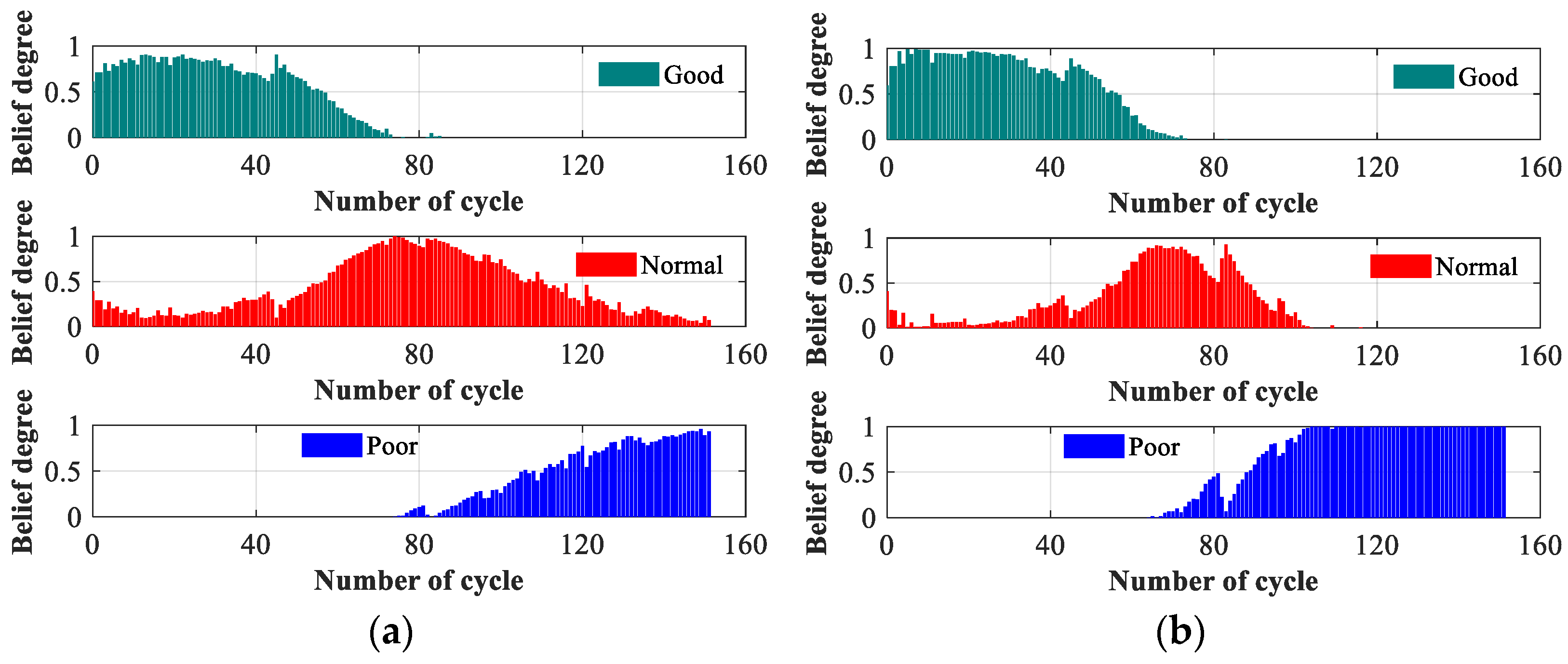
The fused belief distribution can be expressed as follows:

$$e(I)=\{(H_n,p_{n,e(I)}),n=1,\dots ,N,(\Phi ,p_{\Phi ,e(I)})\}$$

(15)

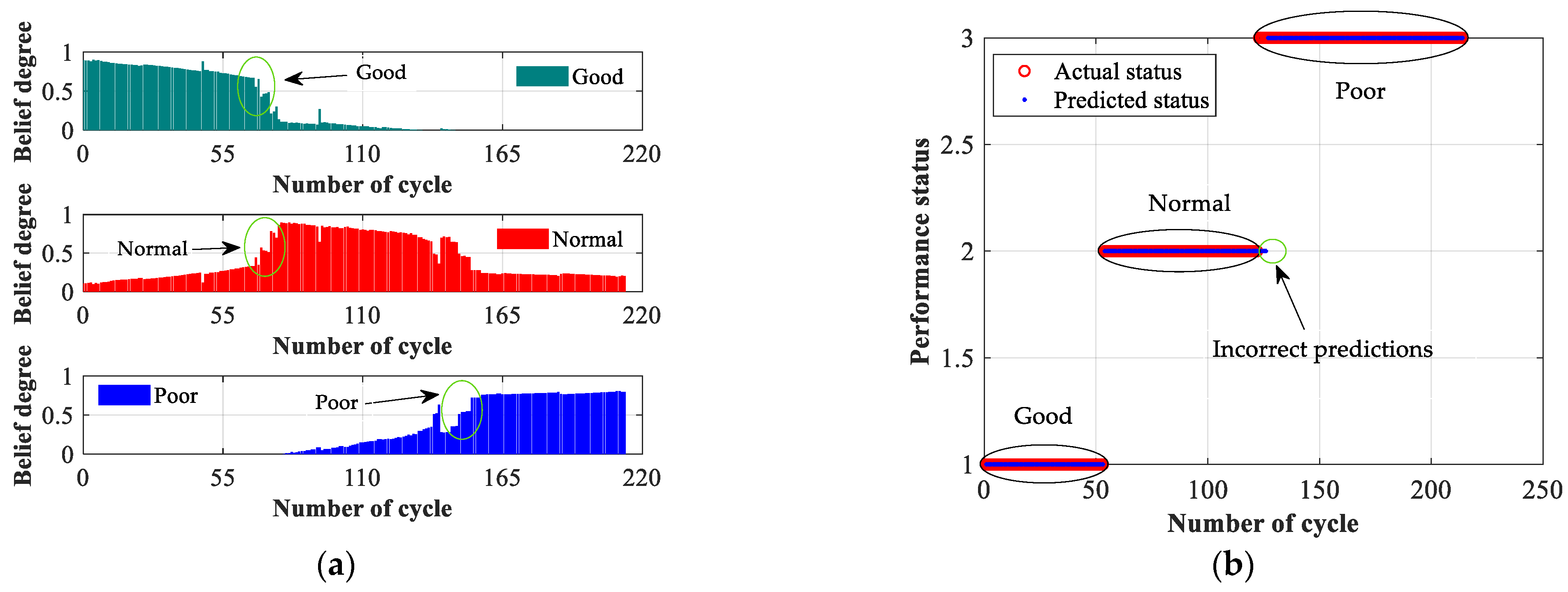
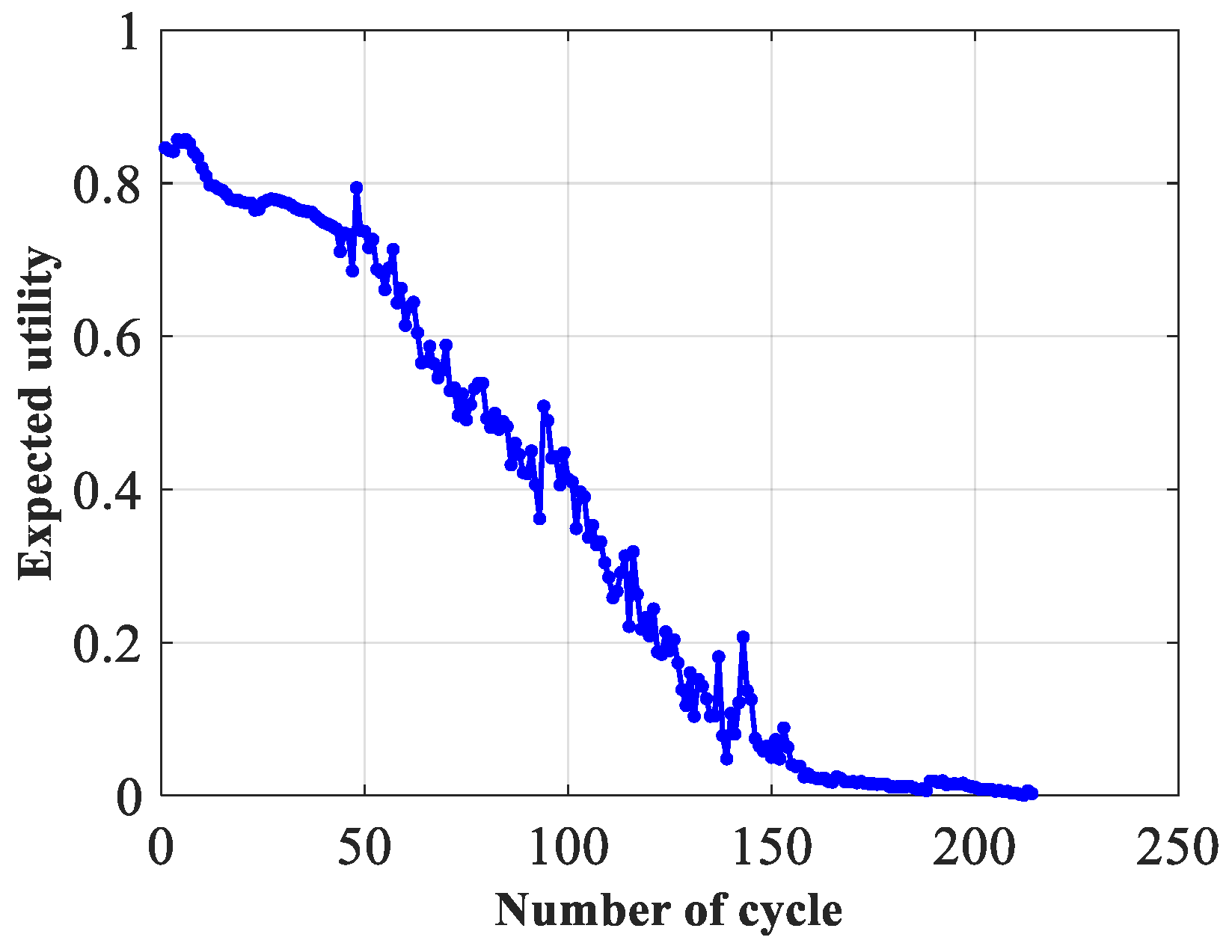
In engineering applications, transforming the belief degree of fused results into expected utility is a useful approach to obtain numerical output results that can be analyzed and interpreted. This transformation allows engineers to quantify the usefulness or value of the fused results, which is essential for decision-making processes.

Once we determine the expected utility values $u(H_n)$ for all assessment levels, we can calculate the expected utility of the fused results [24]. By considering the expected utility, we can effectively evaluate and compare the various health assessment results. The way to express the expected utility $u$ of the health assessment results is as follows:

$$u(e(I))={\displaystyle \sum _{n=1}^{N}u(H_n)p_{n,e(I)}+u(\Phi )p_{\Phi ,e(I)}}$$

(16)

3.5. Optimization of the ER-DRV Model Parameters

The level reference values of indicators play a critical role in determining the aggregate outcome of ER rules [21]. However, the level reference values of indicators are often given by experts, which leads to unreasonable assessment results. Thus, in this section, we introduce an improved whale optimization algorithm (IWOA). The IWOA is designed to optimize the level reference values of the ER-DRV model.

3.5.1. Improved Whale Optimization Algorithm (IWOA)

The purpose of optimizing level reference values is to improve assessment accuracy, which is the objective function of optimization. Thus, based on the WOA, two strategies are proposed in the IWOA.

Strategy 1: Improve the convergence factor.

The global and local search capabilities of the WOA depend on changes in the convergence factors to strike a balance between exploration and exploitation, ultimately improving the algorithm’s optimization efficiency and effectiveness [29]. The convergence factor $a$ in the original WOA linearly decreases from 2 to 0, with the same decreasing speed throughout the entire algorithm. However, the newly designed convergence factor decreases non-linearly, which is more suitable for optimizing the level reference values of the ER-DRV model. An improved nonlinear convergence factor $a$ is displayed in Equation (17) and illustrated in Figure 2a.

$$a=a_{\min }+(a_{\max }-a_{\min })e^{-{(\frac{gt}{T_{\max }})}^4}\alpha$$

(17)

where $a$ denotes the convergence factor, reflecting the speed of convergence, $a_{\min }$ represents the minimum allowable value for the convergence factor, and $a_{\max }$ represents the maximum allowable value that the convergence factor can reach. $g$ is a variable set by expert knowledge, which can change the convergence speed of the convergence factor. $t$ represents the current iteration count, and $T_{\max }$ indicates the maximum number of iterations allowed in the process.

In Figure 2a, it can be seen that the nonlinear convergence factor $a$ decreases nonlinearly with an increasing number of iterations. In the initial stage, the convergence factor $a$ decreases slowly, allowing whales to make larger strides in their movement. This enables them to effectively explore a wide range of possibilities and increase the chance of finding the global optimal solution. However, as the search progresses into the later stage, the convergence factor $a$ decreases rapidly. This means that the whales need to make smaller, more precise strides to fine-tune their search and home in on the optimal solution. Furthermore, it can also be observed that the larger the value of $g$, the greater the decrease in the convergence factor $a$. The smaller the value of $g$, the smaller the decrease in the convergence factor $a$. The value of $g$ should be reasonably set by experts to ensure good experimental results. Overall, this two-stage process allows whales to first explore broadly and then narrow down their search to find the most accurate and optimal solution.

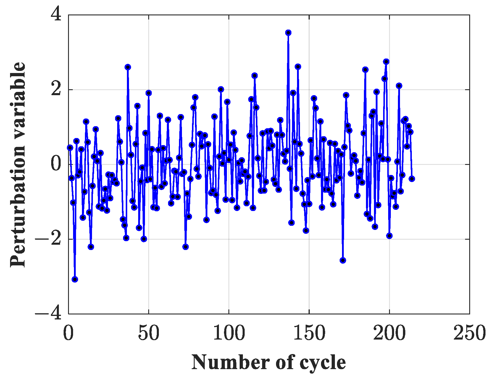
Strategy 2: Disturbances are introduced.

In the prey encirclement stage of the WOA algorithm, the movement of whale individuals is based on the position of the current population leader in the search space, which can easily lead to the algorithm falling into local optima. To enhance the global convergence accuracy of the algorithm and prevent it from becoming stuck in local optima, disturbances $\xi$ with uniform distributions $[-1,1]$ were added after updating the position of whale individuals during the prey encirclement stage. This enhances the algorithm’s ability to overcome local optima and achieve better search optimization in both the initial and final stages. The disturbance formulas are as follows:

$${\varphi }^{\prime }=\varphi +\xi \varphi$$

(18)

$$\xi =\sigma (2z-1)$$

(19)

where $\varphi$ represents a whale individual before a disturbance, ${\varphi }^{\prime }$ represents the whale individual after adding the disturbance, $\sigma$ represents the relative error level set by expert knowledge, where $0\le \sigma \le 1$, and $z$ is a randomly selected number from a uniform distribution $[0,1]$.

The disturbance value obtained increases as the relative error level increases, as shown in Figure 2b. In the experiment, it is necessary to set the relative error level $\sigma$ reasonably to ensure better experimental results.

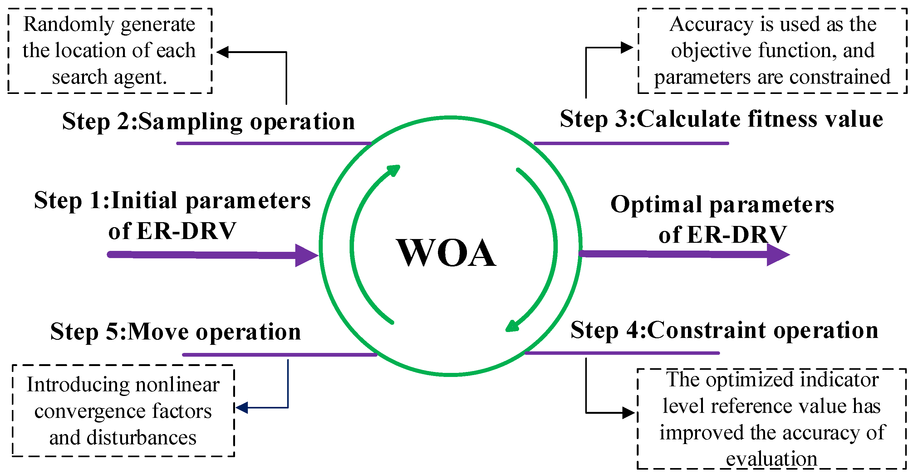
3.5.2. The Optimization Process of the ER-DRV Model’s Parameters

In recent research, various optimization algorithms have been utilized to enhance the health assessment of lithium-ion batteries [6]. Among them, the WOA is used across multiple fields, including classification tasks, robot trajectories, image processing applications, networks, and task scheduling, due to its simplicity of operation, few adjustable parameters, and strong ability to escape local optima [29,30,31].

This article presents an improved version of the WOA, as depicted in Figure 3, with the following specific steps:

Step 1 (Initialization): The variable $n$ represents the initial population of whales. The number of iterations of the search algorithm is denoted by the variable $t$. The maximum number of iterations allowed is denoted by the variable $T_{\max }$. The dimensions of the search space, which represent the number of variables in the optimization problem, are denoted by the variable $d$.

Step 2 (Sample operations): Randomly generate the location of each search agent $Y(t)$.

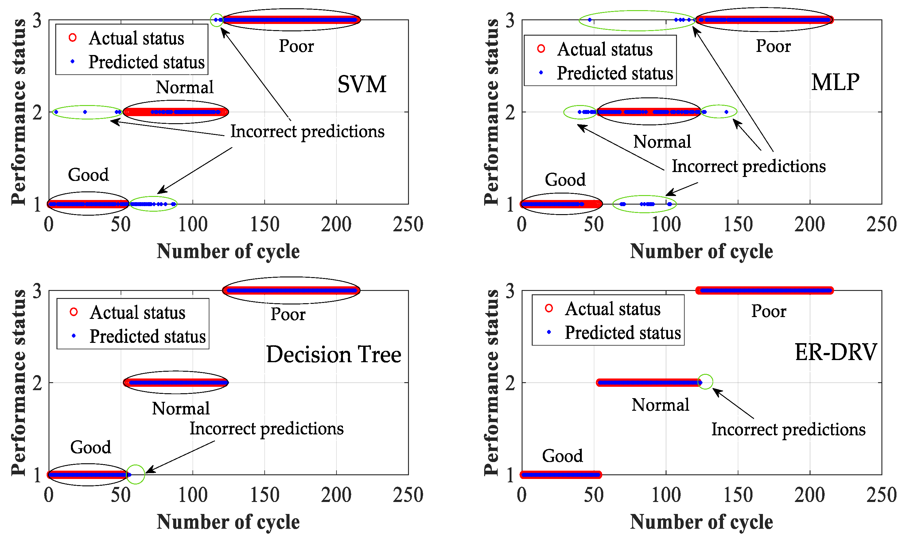
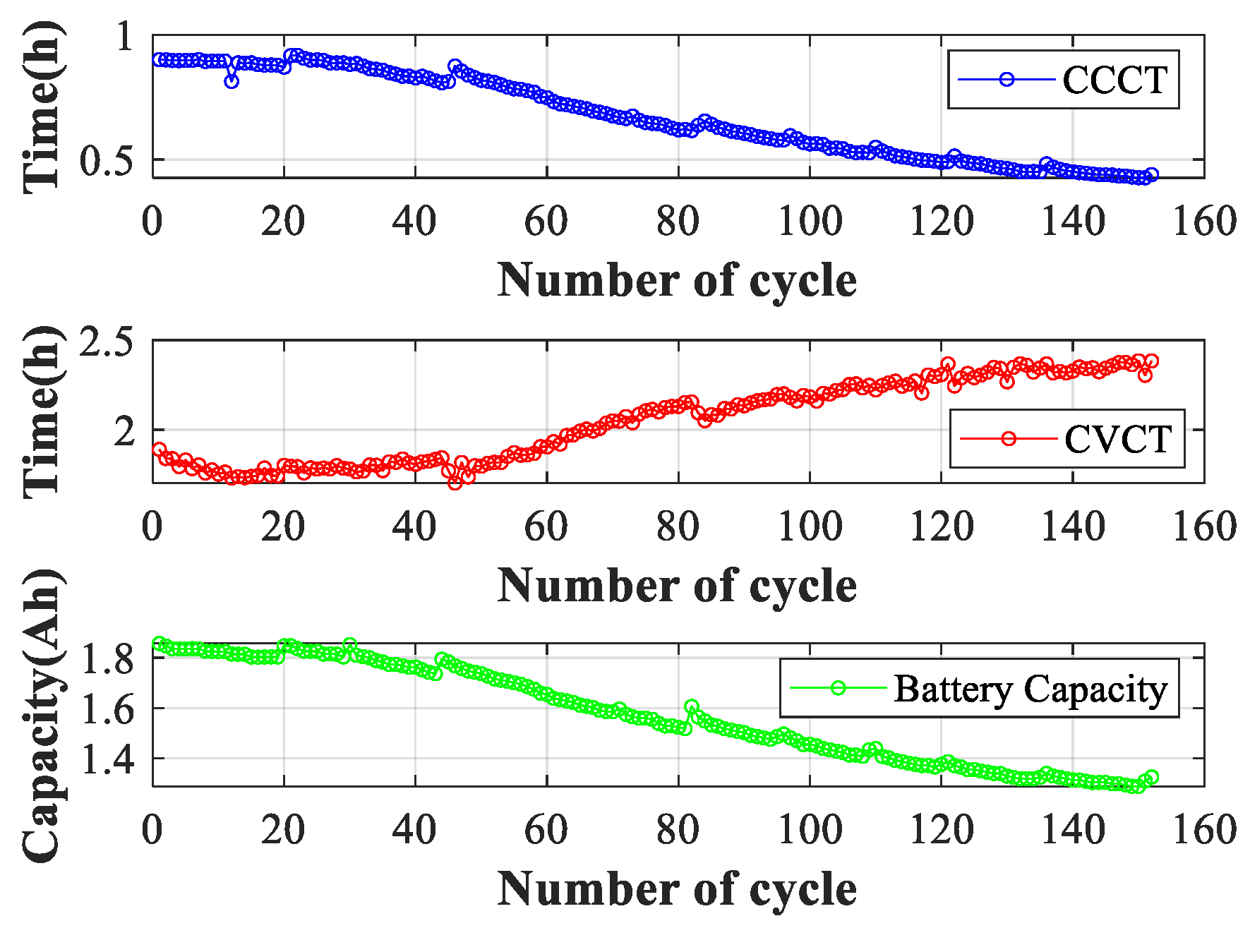
Step 3 (Determine fitness): The objective of this article is to enhance the assessment accuracy of the model. To achieve this, an objective function for optimization was developed and is explained as follows:

$$\begin{gathered} \max (acc({\mu }_{correct},{\mu }_{all}))\mathrm{and}\max ({acc}^{\prime }({{\mu }^{\prime }}_{correct},{{\mu }^{\prime }}_{all})) \\ acc=\frac{{\mu }_{correct}}{{\mu }_{all}}\mathrm{and}{acc}^{\prime }=\frac{{{\mu }^{\prime }}_{correct}}{{{\mu }^{\prime }}_{all}} \end{gathered}$$

(20)

where $acc({\mu }_{correct},{\mu }_{all})$ is the accuracy of the assessment without perturbations. ${\mu }_{correct}$ represents the number of assessed lithium-ion battery statuses that match the actual status. ${\mu }_{all}$ represents the total number of performance statuses. ${acc}^{\prime }({{\mu }^{\prime }}_{correct},{{\mu }^{\prime }}_{all})$ is the accuracy of the assessment under perturbations. ${{\mu }^{\prime }}_{correct}$ represents the number of assessed lithium-ion battery statuses that match the actual status under perturbations. ${{\mu }^{\prime }}_{all}$ represents the total number of the performance statuses under perturbations.

Step 4 (Constraint operation): Combining indicator data and expert knowledge, the upper and lower limits of constraint conditions were set.

$$s.t.\{\begin{array}{l}{C}_{lb}\le c_{1,i},c_{2,i},c_{3,i},\dots ,c_{n,i}\le C_{ub}\\ 0\le z_{i,n}\le m_i\\ i=1,2,\dots ,In=1,2,\dots ,N\end{array}$$

(21)

where $c_{n,i}$ represents the initial level reference value, and $C_{lb}$ and $C_{ub}$ represent the lower and upper bounds of $c_{n,i}$. $m_i$ represents the coefficient that limits excessive overlap between different levels. The values of ($C_{lb}$, $C_{ub}$, $m_i$) are determined by expert knowledge and the observational indicator data.

Step 5 (Exploration and exploitation): When $p<0.5$ and $\left|A\right|<1$, humpback whales can capture prey and surround them. Because the exact location of the optimal solution in the search space is uncertain, the WOA operates under the assumption that the current best candidate solution represents the target prey or is in close proximity to the optimal solution. This assumption helps guide the search toward potentially better solutions and reduces the chances of becoming stuck in suboptimal regions. Once the best search agent is determined, other search agents strive to adjust their positions to match that of the best search agent. This process is described by the following two formulas:

$$G=\left|C{Y}_{best}(t)-Y(t)\right|$$

(22)

$$Y(t+1)=Y_{best}(t)-AG$$

(23)

where $A$ and $C$ denote the coefficient vector, the current whale’s position can be expressed as vector $Y(t)$, and $t$ represents the current iteration number. The vectors $A$ and $C$ can also be expressed using the following equation:

$$A=2a\nu -a,C=2\nu$$

(24)

$$a=2-2t/T_{\max }$$

(25)

where $\nu$ is a random vector on the interval $[0,1]$. $T_{\max }$ represents the upper limit of the number of iterations, and the linear convergence factor of the WOA can be expressed as $a$. To improve the balance between exploration and exploitation in optimizing the ER-DRV model, a transformation is applied to convert $a$ into a convergent decreasing form that is nonlinear.

To prevent the WOA from becoming trapped in local optima during optimization, random disturbances are introduced. This process is described in (18) and (19).

When $p<0.5$ and $\left|A\right|\ge 1$, humpback whales exhibit a unique foraging behavior that can be described as “randomly searching for prey”. This process can also be expressed using the following equation:

$$G=\left|C{Y}_{rand}(t)-Y(t)\right|$$

(26)

$$Y(t+1)=Y_{rand}(t)-AG$$

(27)

where $Y_{rand}(t)$ denotes the position of randomly selected whales. When $\left|A\right|\ge 1$, the positions of other whales are updated based on the randomly selected whale positions, forcing the whales to stay away from their prey and find more suitable prey. This can enhance the algorithm’s exploration ability and enable the WOA to conduct global searches.

When $p\ge 0.5$, humpback whales use a distinct hunting strategy in which they encircle their prey in a spiral formation of bubbles. They then utilize a spiral contraction approach to efficiently capture their intended target. This process can be represented by the following formula:

$$Y(t+1)=Y_{best}(t)+G_p{e}^{bl}\cos (2\pi l)$$

(28)

$$G_p=\left|Y_{best}(t)-Y(t)\right|$$

(29)

where $G_p$ represents the distance separating a humpback whale from its prey, $b$ denotes the constant of the spiral motion trajectory, and $l$ represents random numbers between intervals $[-1,1]$.

4. Perturbation Analysis

Ho et al. introduced perturbation analysis in their study of discrete event dynamic systems [32]. It is a method used in various fields, such as mathematics, physics, economics, and biology, to study the behavior of a system when it undergoes a small change or perturbation. Its characteristic is that the trajectory of perturbed samples is not obtained using other simulations or experiments but is constructed using theoretical analysis methods based on nominal sample trajectories. Perturbation analysis is a method used to evaluate the effectiveness of an ER rule by examining its behavior under perturbations in the input data [25]. This analysis helps to understand how the model responds to small perturbations and provides insights into its robustness and stability.

4.1. Definition of Perturbation

During the operation of lithium-ion batteries, they may experience perturbations that can lead to various changes in the observed indicator data. To carry out perturbation analysis, as shown in Formula (3) and Figure 1, two important variables are defined: the perturbation intensity $\tau$ and the perturbation variable $\Delta x(k)$. The perturbation variable is random and follows a normal distribution.

The perturbed indicator data are obtained by adding perturbations to the original indicator data.

$$X_i^{\prime }(k)=X_i(k)+\tau \times \Delta x(k)$$

(30)

where $X_i^{\prime }(k)$ represents the data of observation indicator $i$ in the $k\text{-}\mathrm{th}$ cycle under perturbed conditions, $X_i(k)$ represents the data for the observed indicator $i$ without perturbation conditions, and $k=1,2,\dots ,K$. Under perturbation conditions, the input indicator $X_i(k)$ becomes $X_i^{\prime }(k)$, and $X_i^{\prime }(k)$ is equal to $X_i(k)+\tau \times \Delta x(k)$. The process of ER rule fusion under perturbation conditions is illustrated in Figure 4.

The upper part of Figure 4 shows the standard sample with the input parameter $X_i$, which is fused with an ER to obtain $PM(X_i)$. The lower part is the perturbed sample, where the input parameter changes from $X_i$ to $X_i+\tau \Delta x_i$, and $PM(X_i+\tau \Delta x_i)$ is obtained using ER fusion. According to reference [25], $PM(X_i)$ and $PM(X_i+\tau \Delta x_i)$ can be regarded as equivalent to the expected utility $u$ and $u^{\prime }$.

In Section 3.4, the input indicator can be represented as $X_i(i=1,\dots ,I)$, and the evidence can be represented as $e_i(i=1,\dots ,I)$. The number of reference levels is $N$, represented by $\Phi =\{H_1,\dots ,H_N\}$. Under perturbation conditions, the reliability and weight of indicators are represented as $\{r^{\prime }{}_1,r^{\prime }{}_2,\dots ,r^{\prime }{}_I\}$ and $\{{\omega }^{\prime }{}_1,{\omega }^{\prime }{}_2,\dots ,{\omega }^{\prime }{}_I\}$, respectively. The calculation of the belief distribution of the evidence $e_i$ is completed using Formula (15).

$$e_i=\{(H_l,\frac{X_i^{\prime }-h_{l+1}}{h_l-h_{l+1}}),(H_{l+1},\frac{h_l-X_i^{\prime }}{h_l-h_{l+1}}),(H_{\nu },0)\}$$

(31)

where $\nu \in [1,N]$, $\nu \ne l,l+1$. Similarly, we can also obtain the belief distribution of the evidence $e_j$. ER rules are used to fuse all indicators and yield accurate results for health assessments. Using Formula (16), the expected utility $u^{\prime }$ can be obtained.

4.2. The Reasoning Process of Perturbation Analysis

Based on [19,25], it is assumed that there are $L$ independent pieces of evidence and $M$ pieces of perturbation evidence $\{e_1,\dots ,e_i,\dots ,e_M,e_{M+1},\dots ,e_j,\dots ,e_L\}$. The process of perturbation analysis is divided into the following two steps:

• Step 1: Based on the ER rule in (12)–(14), the first $(L-M)$ pieces of evidence without perturbation are fused with weight and reliability, and then $e(L-M)$ is calculated using (15).
• Step 2: Based on the ER rule, the previous assessment result $e(L-M)$ is mixed with the first perturbation piece of evidence to obtain $e(L-M+1)$. Subsequently, the expected utility $u(X_1)$ and perturbed expected utility $u(X_1+\tau \Delta x_1)$ are calculated using (16).
• Step 3: Repeat the ER rule in step 1 and combine $e(L-M+1)$ in step 2 with the remaining $(M-1)$ pieces of evidence to obtain the expected utility.

5. Case Study

5.1. Research Background

The experimental data were collected from the 18650 lithium-ion battery public dataset of the Hawaii Natural Energy Institute (HNEI) [33]. These batteries have a nominal capacity of 2.8 Ah and underwent 1000 cycles of charging at 0.5 C and discharging at 1.5 C at room temperature (25 °C). Each cycle in the dataset contains many characteristic indicators, such as charging time, discharge time, maximum voltage, minimum voltage, remaining useful life, etc. Therefore, both the data size and characteristic indicators of the dataset from the HNEI meet the requirements for lithium-ion battery health state assessment. The data marked as 25C_0-100_0.5/1.5C_P’s battery were extracted as observation indicators. According to expert knowledge, the health states of batteries were set to “good”, “normal”, and “poor”. When the actual capacity of a lithium battery was greater than 90% of its nominal capacity, it was considered “good”. When the actual capacity reached 85% of the nominal capacity, it was considered “normal”, and when the actual capacity decayed to 80% of the nominal capacity, it was considered “poor”. At this point, the battery reaches EOP (End of Performance), and its capacity and performance significantly decrease, making it unable to meet the requirements of the application [34]. Finally, 214 pieces of data were obtained.

Constant current charging time $X_{cc}$, constant voltage charging time $X_{cv}$, and voltage drop time from 3.6 V to 3.4 V $X_d$ were selected as observation indicators. Moreover, $X_{cc}$, $X_{cv}$, and $X_d$ are replaced with CCCT, CVCT, and DT, respectively, in the following.

As depicted in Figure 5a, it can be observed that there is a declining trend in the values of CCCT, CVCT, and DT with an increase in the number of cycles. The smaller the values of the three indicators, the poorer the health state of the battery. In Figure 5b, the capacity of the battery shows a decreasing trend. The capacity fluctuates slightly at 24, 48, 71, 117, 164, and 211 cycles and fluctuates significantly at 94, 141, and 189 cycles, indicating unstable battery performance at this time.

5.2. Health State Assessment of Lithium-Ion Batteries Based on ER Rules

In this section, three reference levels are set, including “good”, “normal”, and “poor”. Referring to the identification framework $\Phi =\{H_1,\dots ,H_N\}$ in Section 3.4, $\Phi =\{(H_1,\mathrm{good}),(H_2,\mathrm{normal}),(H_3,\mathrm{poor})\}$ is obtained. According to expert knowledge, the “good” and “poor” reference values for CCCT, CVCT, and DT in

Table 1. The health levels and level reference values of indicators.

Indicators (Hour)	${\mathit{H}}_1$ (Good)	${\mathit{H}}_2$ (Normal)	${\mathit{H}}_3$ (Poor)
CCCT	1.7224	1.5523	1.4023
CVCT	1.4564	1.2607	1.1434
DT	0.2473	0.2014	0.1735

are the maximum and minimum values observed in the dataset [19,35], respectively. Additionally, the “normal” reference value is determined by the data corresponding to the 109th cycle.

From Table 1, it can be seen that when CCCT is equal to 1.7224, the battery has a “good” performance at this time. As the number of cycles increases, the value of CCCT also decreases, indicating that the performance of the battery gradually deteriorates until the battery’s actual capacity decays to 80% of the nominal capacity, and the battery reaches its EOP [34]. It is considered that the state of the battery is “poor” at this time, and CCCT is equal to 1.4023. For CVCT and DT, the principle is also the same.

To monitor the health state of the battery in real time, the real-time reliability of the evidence was obtained using Formulas (4)–(7), as shown in Figure 6a. Using Formulas (8) and (9), the real-time weights of the evidence were obtained, as shown in Figure 6b.

In Figure 6a, the reliability of the three indicators is continuously updated as the number of cycle increases. The reliability of indicator “CCCT” has small fluctuations during the early cycles, experiences significant fluctuations between the 50th and 150th cycles, and becomes stable after the 150th cycle. The indicator “CVCT” exhibits a decrease in reliability from the 1st cycle to the 50th cycle, followed by small fluctuations from the 50th cycle to 150th cycle, and becomes stable after the 150th cycle. The reliability of indicator “DT” only shows some fluctuations in the early stage and then follows a downward trend for the remaining cycles.

In Figure 6b, the weight of indicator “CCCT” has small fluctuations in the early cycles and then follows an upward trend for the remaining cycles. The trend in the indicator “CVCT” is similar to the trend in the indicator “CCCT”. The weight of indicator “DT” only shows some fluctuations in the early stage, and then follows a downward trend for the remaining cycles.

It can be inferred from the above analysis that real-time reliability and real-time weight are more capable of reflecting the true condition of the data compared with static reliability and static weight.

Using Formulas (10) and (11), the belief distributions of three observation indicators were obtained. The parameters were fused using Formulas (12) to (15) to generate the health assessment results, as illustrated in Figure 7a.

Figure 7a illustrates trends in the belief degrees. Specifically, the “good” belief degree demonstrates a continuous decline from the 1st cycle to the 110th cycle. On the other hand, the “normal” belief degree peaks at the 107th cycle and remains mostly concentrated between the 55th and 165th cycles. In contrast, the “poor” belief degree starts to show an increasing trend after the 110th cycle. The health state of the battery depends on the “good” belief degree at the initial stage of the cycle, followed by the “normal” belief degree at the middle stage, and then the “poor” belief degree at the end. This suggests that with an increase in the number of cycles, the battery’s actual capacity decreases, leading to a deteriorating health state.

According to the definitions of “good”, “normal”, and “poor” for the three health states of lithium-ion batteries in Section 5.1, the 214 pieces of data are divided into three categories: 1 represents “good”, 2 represents “normal”, and 3 represents “poor”.

As shown in Figure 7b and

Table 2. Comparison of actual results and predicted results of lithium-ion batteries.

Performance Status	${\mathit{H}}_1$ (Good)	${\mathit{H}}_2$ (Normal)	${\mathit{H}}_3$ (Poor)
Predicted results	1–53	54–158	159–214
Actual results	1–53	54–122	123–214

, at the critical points of “normal” and “poor”, which are 123–158 cycles, there are still some incorrect predictions. This is due to the use of initial expert knowledge to set level reference values. Thus, the assessment accuracy of the methods used in this section is 83.18%.

It is possible to translate belief distribution into numerical output using expected utility. By defining the utility of the reference level as $u(H_1)=1$, $u(H_2)=0.5$, and $u(H_3)=0$, we can determine the expected utility using Formula (16). In Figure 8, the expected utility depicts a consistent decline. It fluctuates slightly at 25, 71, 117, 166, and 213 cycles and fluctuates greatly at 48, 94, 142, and 189 cycles, indicating an unstable health state at these moments. The trend in the expected utility is somewhat similar to the battery’s capacity shown in Figure 5b. This indicates that the health assessment method proposed in this section has certain effectiveness.

5.3. Health State Assessment of Lithium-Ion Batteries Using the ER-DRV Model

In Section 5.2, the level reference values of the observation indicators are set by experts, resulting in inaccurate health assessment results. Therefore, in order to improve the accuracy of the model, the improved whale algorithm (IWOA) was used in the ER-DRV model to optimize the level reference values within reasonable constraints. According to Equations (20) and (21), the objective function and constraints of the indicator reference values are as follows:

$$\begin{array}{ll}& \max (acc({\mu }_{correct},{\mu }_{all}))\\ s.t.& \{\begin{array}{l}1.7\le c_{1,1}\le 2.7,1.48\le c_{2,1}\le 1.7,0.4\le c_{3,1}\le 1.48\\ 1.42\le c_{1,2}\le 1.9,1.22\le c_{2,2}\le 1.42,0.25\le c_{3,2}\le 1.22\\ 0.21\le c_{1,3}\le 0.30,0.19\le c_{2,3}\le 0.21,0.08\le c_{3,3}\le 0.19\\ 0\le z_{1,1},z_{2,1},z_{3,1}\le 1;0\le z_{1,2},z_{2,2},z_{3,2}\le 1;0\le z_{1,3},z_{2,3},z_{3,3}\le 1;\end{array}\end{array}$$

(32)

The level reference values of the indicators optimized using the IWOA are shown in

Table 3. Indicator health levels and level reference values after IWOA optimization.

Indicators (Hour)	${\mathit{H}}_1$ (Good)	${\mathit{H}}_2$ (Normal)	${\mathit{H}}_3$ (Poor)
CCCT	2.0279	1.6878	1.4680
CVCT	1.8975	1.3992	1.2084
DT	0.2210	0.2000	0.1800

. Based on the optimized reference values, a new comprehensive belief distribution for lithium-ion batteries was obtained, as shown in Figure 9a.

In Figure 9a, the “good” belief degree demonstrates a continuous and slow declining trend from the 1st cycle to the 70th cycle. Moreover, the “normal” belief degree peaks at the 78th cycle and remains mostly concentrated between the 74th and 145th cycles. In contrast, the “poor” belief degree starts to show a stable trend after the 153rd cycle. According to the results presented above, it can be seen that the health assessment results of lithium-ion batteries optimized with the IWOA are more accurate and in line with reality.

In Figure 9b, the accuracy of the health assessment of lithium batteries optimized with the IWOA is as high as 99.53%, which is significantly better than the accuracy of 83.18% in Figure 7b. It can be seen that the IWOA greatly improves the assessment accuracy of the model by optimizing level reference values.

The expected utility can be calculated using Formula (16), and the trend in the utility change after IWOA optimization is shown in Figure 10.

In Figure 10, the expected utility shows a gradual decreasing trend. The expected utility fluctuates slightly at 24, 57, 62, 70, 116, 153, and 189 cycles and fluctuates greatly at 48, 94, 137, and 143 cycles, indicating an unstable health state at this time. The initial expected utility in Figure 10 is 0.85, instead of the expected utility of 1 in Figure 8. The initial battery capacity in Figure 5b is 2.63 Ah, not the nominal capacity of 2.8 Ah. Therefore, compared with Figure 8, the expected utility in Figure 10 is closer to the capacity trend in the battery in Figure 5b.

The main parameters that affect the optimization effect of the WOA include the number of iterations and the populations. Generally, the more iterations and the larger the number of populations, the stronger the optimization ability of the WOA becomes. To further verify the impact of different parameters on the optimization effects of the WOA and IWOA, relevant experiments were conducted. The variable dimensions of the WOA and IWOA were set to 9, and the number of iterations $t$ and population $n$ are shown in

Table 4. Accuracy of health assessments using WOA optimization with different parameters.

Accuracy of Assessment	$\mathit{n}$ = 20	$\mathit{n}$ = 30	$\mathit{n}$ = 50	$\mathit{n}$ = 70
$t$ = 10	92.52%	93.46%	94.86%	95.79%
$t$ = 30	93.46%	94.86%	95.33%	95.79%
$t$ = 50	95.33%	95.33%	95.33%	96.73%
$t$ = 100	95.33%	95.79%	95.79%	95.33%

and

Table 5. Accuracy of health assessments using IWOA optimization with different parameters.

Accuracy of Assessment	$\mathit{n}$ = 20	$\mathit{n}$ = 30	$\mathit{n}$ = 50	$\mathit{n}$ = 70
$t$ = 10	97.66%	98.06%	99.07%	99.07%
$t$ = 30	98.13%	99.07%	99.53%	99.13%
$t$ = 50	97.66%	99.07%	99.53%	99.53%
$t$ = 100	99.53%	99.53%	99.53%	99.53%

. From the two tables, it can be seen that under the same population size and iteration number, the IWOA enables the model to have higher assessment accuracy. The experiments were conducted with a population size of 50 and a maximum iteration of 30.

To further support the benefits of the IWOA, comparative studies were carried out, comparing it with other popular machine learning techniques such as Support Vector Machine (SVM), Multilayer Perceptron (MLP), and Decision Tree. Sixty percent of the observation samples were used for training, and all observation samples were used for testing.

As shown in Figure 11, SVM and MLP made many incorrect predictions as “good”, “normal”, and “poor”; the Decision Tree made a few incorrect predictions, while the ER-DRV model made very few incorrect predictions.

The assessment accuracy of the different models is shown in

Table 6. Assessment accuracy of different models.

NO.	Model	Accuracy of Assessment
1	ER	83.18%
2	ER-WOA	95.33%
3	ER-DRV	99.53%
4	Decision Tree	96.24%
5	MLP	85.94%
6	SVM	84.51%

. The accuracy of the ER-DRV model proposed in this article reaches 99.53%, which is higher than that of the other models. This indicates that compared with the other methods, the ER-DRV model effectively improves assessment accuracy. In addition, the clear and transparent reasoning process of ER rules holds significant practical value in engineering applications.

5.4. Robustness Analysis of the ER-DRV Model

To further analyze the robustness of the ER-DRV model, a perturbation analysis method was used to simulate environmental perturbations.

Assume there are six types of perturbations, namely, low-frequency vibration and high temperature, high-frequency vibration and high temperature, low-frequency vibration and normal temperature, high-frequency vibration and normal temperature, low-frequency vibration and low temperature, and high-frequency vibration and low temperature. The perturbation intensities $\tau$ are 0.00150, 0.00155, 0.00160, 0.00165, 0.00170, and 0.00175, respectively. Additionally, it is important to ensure that perturbations do not heavily influence the observation indicators. Therefore, the intensity of the perturbations should be determined in a practical manner that accurately simulates real-life perturbation conditions. In Figure 12, the perturbation variables are presented.

The perturbation was incorporated into the original indicator data by introducing a random number that follows a normal distribution. Thus, each observation indicator was recalculated, resulting in changes in the reliability, weight, and level reference values. The real-time weight and real-time reliability calculation under different perturbation intensities were completed using Formulas (4)–(9). The upper and lower limits of constraints were redefined, and the dynamic level reference value was obtained using IWOA optimization. The optimized dynamic level reference values are shown in

Table 7. Level reference values after IWOA optimization under six perturbation intensities.

Observed Indicators (Hour)	Perturbation Intensities	${\mathit{H}}_1$ (Good)	${\mathit{H}}_2$ (Normal)	${\mathit{H}}_3$ (Poor)	Perturbation Intensities	${\mathit{H}}_1$ (Good)	${\mathit{H}}_2$ (Normal)	${\mathit{H}}_3$ (Poor)
CCCT	0.00150	2.1424	1.5926	1.1193	0.00155	2.2000	1.6900	1.4700
CVCT		1.6234	1.3368	1.2092		1.4661	1.4100	1.2100
DT		0.2200	0.2162	0.1890		0.2203	0.1988	0.1873
CCCT	0.00160	2.2000	1.6723	1.4700	0.00165	2.2000	1.6258	1.2068
CVCT		1.4565	1.3027	0.6707		1.4200	1.3071	1.2100
DT		0.2216	0.2134	0.1890		0.2207	0.2150	0.1890
CCCT	0.00170	1.8440	1.5798	1.2009	0.00175	1.8336	1.5573	1.4678
CVCT		1.4200	1.3839	1.1566		1.6988	1.4096	1.0992
DT		0.2217	0.2133	0.1890		0.2218	0.2114	0.1888

.

The assessment accuracy of the ER-DRV model under six perturbation intensities is shown in

Table 8. Assessment accuracy of the ER-DRV model under six perturbation intensities.

NO.	Perturbation Intensities	Accuracy
1	0.00150	98.79%
2	0.00155	98.13%
3	0.00160	97.66%
4	0.00165	97.66%
5	0.00170	97.66%
6	0.00175	97.66%

. As the perturbation intensity increases, the accuracy decreases slightly. However, the assessment accuracy of the ER-DRV model under perturbations is still higher than the assessment accuracy of the other models without perturbations in Table 6. The experimental results demonstrate that the use of dynamic reference values, real-time weights, and real-time reliability can improve the assessment accuracy and robustness of the ER-DRV model.

In Figure 13, when the perturbation intensity increases, the expected utility has a slight difference. The expected utility in Figure 13 has a similar fluctuation trend, with large fluctuations at cycles 48, 94, 137, and 143 and small fluctuations at cycles 24, 57, 62, 70, 116, and 153. This fluctuation trend is basically consistent with the trend without perturbation in Figure 10. This suggests that the ER-DRV model is capable of accurately evaluating the overall condition of batteries even when they are subjected to perturbations. Moreover, the ER-DRV model is robust and can integrate indicators with added perturbations to obtain reasonable assessment results.

5.5. Additional Experiment

5.5.1. Health State Assessment

To further demonstrate the validity and generalization ability of the proposed method, a case from the lithium-ion battery dataset obtained from the data repository of the NASA Ames Prognostics Center of Excellence [36] is studied.

The experiment takes place at room temperature and follows a specific set of procedures. During the charging process, the battery is charged in a constant current mode at a rate of 1.5 A. The charging continues until the battery voltage reaches 4.2 V. Once the voltage reaches this level, the charging mode switches to constant voltage mode. This mode is maintained until the charge current drops to 20 mA. The discharging process, on the other hand, is carried out at a constant current level of 2 A. The battery is discharged until the voltage falls to 2.7 V. The experiments are stopped when the batteries reach the end-of-life (EOL) criteria. The EOL criteria is defined as a 30% fade in rated capacity, which means the battery’s capacity decreases from 2 Ah to 1.4 Ah. It is important to note that the data used in this case study is from battery #5.

Constant current charging time (CCCT) and constant voltage charging time (CVCT) were selected as observation indicators. The observation indicators and capacity of the battery are shown in Figure 14.

The “good”, “normal”, and “poor” reference values for CCCT and CVCT, as shown in

Table 9. Indicator health levels and level reference values.

Indicators (Hour)	${\mathit{H}}_1$ (Good)	${\mathit{H}}_2$ (Normal)	${\mathit{H}}_3$ (Poor)
CCCT	0.9190	0.6479	0.4120
CVCT	1.6852	2.1058	2.3990

, were determined by experts.

Table 10. Indicator health levels and level reference values after IWOA optimization.

Indicators (Hour)	${\mathit{H}}_1$ (Good)	${\mathit{H}}_2$ (Normal)	${\mathit{H}}_3$ (Poor)
CCCT	0.9350	0.6520	0.5421
CVCT	1.7910	1.9921	2.2113

shows the “good”, “normal” and “poor” reference values for CCCT and CVCT determined using the IWOA.

In Figure 15a, the reliability of the two indicators shows an overall upward trend as the number of cycles increases. In Figure 15b, the weight of the two indicators shows some fluctuations in the early stage and then follows a stable trend for the remaining cycles. This is because the IWOA was used to optimize the level reference values, improving the belief degree of the health assessment model. Thus, we did not compare weight and reliability before and after IWOA optimization.

Figure 16 shows the belief degree before and after IWOA optimization. The health status of the battery depends on the “good” belief degree at the initial stage of the cycle, followed by the “normal” belief degree at the middle stage of the cycle, and then the “poor” belief degree at the end of the cycle. It can be seen that the health assessment results after optimization with the IWOA in Figure 16 are more precise.

To further support the advantages of the IWOA, comparative studies were carried out, comparing it with ER, ER-WOA, SVM, MLP, and Decision Tree.

The accuracy of the different models is shown in

Table 11. Comparison of assessment accuracy of the different models.

NO.	Model	Accuracy of Assessment
1	ER	84.87%
2	ER-WOA	96.71%
3	ER-DRV	98.03%
4	Decision Tree	97.35%
5	MLP	95.36%
6	SVM	94.04%

. The accuracy of the ER-DRV model proposed in this article reaches 98.03%, which is higher than that of the other models. This indicates that not only is its reasoning process transparent and interpretable, but it also has good generalization ability and effectiveness.

5.5.2. Robustness Analysis

To further analyze the robustness and generalization ability of the proposed model, assume there are four types of perturbations. The perturbation intensities are 0.00150, 0.00155, 0.00160, and 0.00165. The observation indicators are recalculated under perturbations, resulting in changes in the level reference values, weight, and reliability. The dynamic level reference values after IWOA optimization under perturbations are shown in

Table 12. Level reference values after IWOA optimization under four perturbation intensities.

Observed Indicators (Hour)	Perturbation Intensities	${\mathit{H}}_1$ (Good)	${\mathit{H}}_2$ (Normal)	${\mathit{H}}_3$ (Poor)	Perturbation Intensities	${\mathit{H}}_1$ (Good)	${\mathit{H}}_2$ (Normal)	${\mathit{H}}_3$ (Poor)
CCCT	0.00150	0.9200	0.6799	0.5827	0.00155	0.9400	0.6600	0.5500
CVCT		1.7500	2.1167	2.1325		1.8300	2.1512	2.1823
CCCT	0.00160	0.9428	0.6785	0.5420	0.00165	0.9425	0.6714	0.5539
CVCT		1.7535	2.1230	2.1680		1.8385	2.1552	2.1822

.

Perturbation primarily affects the reliability and weights of indicators. Thus, we conducted an analysis of reliability and weight under perturbation conditions. From Figure 15, Figure 17 and Figure 18, it can be seen that there is little change in the weights and reliabilities after perturbation. This indicates that the ER-DRV model has a good ability to resist perturbations.

From Figure 19, it is evident that the degree of belief is somewhat influenced by four perturbations, but the overall impact is not significant.

Table 13. Assessment accuracy of the ER-DRV model under four perturbation intensities.

NO.	Perturbation Intensities	Accuracy
1	0.00150	96.05%
2	0.00155	96.05%
3	0.00160	96.05%
4	0.00165	96.05%

shows the accuracy of the assessment model under perturbations. The ER-DRV model has an assessment accuracy rate of 98.03% without perturbations. However, the assessment accuracy decreases to 96.05% under perturbations. This may be due to the impact of perturbations on the weight, reliability, and belief degree, ultimately affecting the assessment results and assessment accuracy. In conclusion, the experiment shows that the ER-DRV model under perturbation conditions not only has high accuracy but also has good generalization ability and robustness.

6. Conclusions

In this article, a health assessment model based on evidence reasoning rules with dynamic reference values for lithium-ion batteries is proposed. Meanwhile, an improved WOA method is used to optimize the level reference value of the model for improving assessment accuracy. Moreover, the robustness of the model was studied using perturbation analysis methods. The effectiveness and generalization ability of the model is illustrated using two open lithium-ion battery datasets as examples.

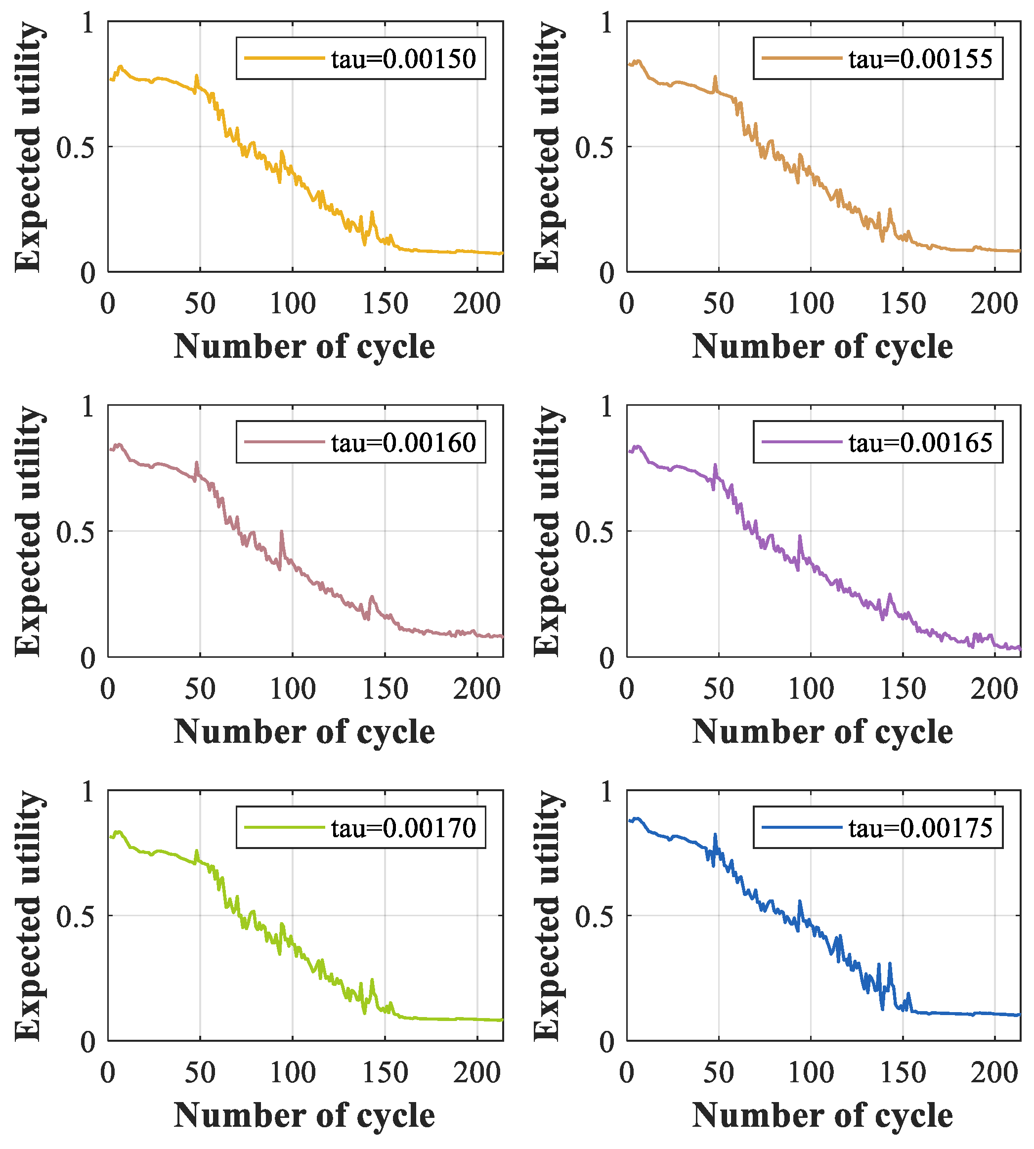
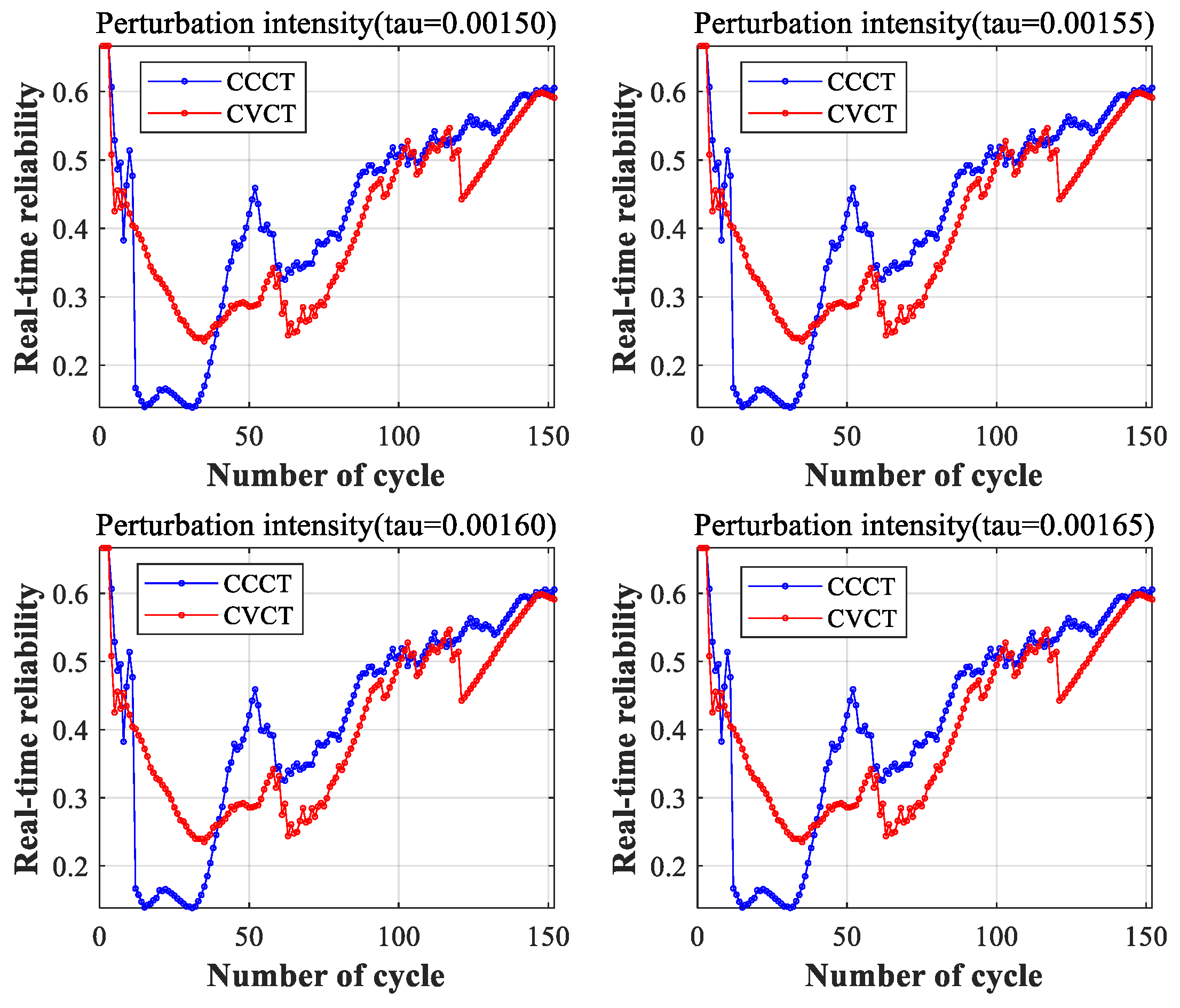
There are three main contributions of this paper. Firstly, the nonlinear convergence factor and disturbances are introduced into the WOA, and an improved WOA is proposed for optimizing level reference values. Secondly, the distance-based method and the coefficient of variation method are used to obtain real-time reliability and real-time weight. Then, the IWOA is used to obtain dynamic level reference values. Therefore, the accuracy of the model assessment is improved. Thirdly, to study the robustness of the ER-DRV model, perturbation variables and perturbation intensities are added to the observation indicators. Using experiments, it was found that perturbations can lead to a decrease of about 2% in model’s accuracy. The experimental results demonstrate that the proposed ER-DRV model effectively evaluates the health state of lithium-ion batteries. Furthermore, it exhibits remarkable robustness and generalization capability.

In the future, it is necessary to develop a reasonable method to reduce the impact of perturbation on the assessment results and improve assessment accuracy. It is important to focus future work on addressing these challenges.

References

1. Zhang, Q.; Wang, D.; Schaltz, E.; Stroe, D.-I.; Gismero, A.; Yang, B. Lithium-ion battery calendar aging mechanism analysis and impedance-based State-of-Health estimation method. J. Energy Storage 2023, 64, 107029. [Google Scholar] [CrossRef]
2. Zhang, C.; Zhao, S.; Yang, Z.; Chen, Y. A reliable data-driven state-of-health estimation model for lithium-ion batteries in electric vehicles. Front. Energy Res. 2022, 10, 1013800. [Google Scholar] [CrossRef]
3. Lin, Z.; Cai, Y.; Liu, W.; Bao, C.; Shen, J.; Liao, Q. Estimating the state of health of lithium-ion batteries based on a probability density function. Int. J. Electrochem. Sci. 2023, 18, 100137. [Google Scholar] [CrossRef]
4. Diao, W.; Saxena, S.; Pecht, M. Accelerated cycle life testing and capacity degradation modeling of LiCoO2-graphite cells. J. Power Sources 2019, 435, 226830. [Google Scholar] [CrossRef]
5. Ren, X.; Liu, S.; Yu, X.; Dong, X. A method for state-of-charge estimation of lithium-ion batteries based on PSO-LSTM. Energy 2021, 234, 121236. [Google Scholar] [CrossRef]
6. Ge, M.-F.; Liu, Y.; Jiang, X.; Liu, J. A review on state of health estimations and remaining useful life prognostics of lithium-ion batteries. Measurement 2021, 174, 109057. [Google Scholar] [CrossRef]
7. Yang, J.; Xia, B.; Huang, W.; Fu, Y.; Mi, C. Online state-of-health estimation for lithium-ion batteries using constant-voltage charging current analysis. Appl. Energy 2018, 212, 1589–1600. [Google Scholar] [CrossRef]
8. Zhang, X.; Gao, Y.; Guo, B.; Zhu, C.; Zhou, X.; Wang, L.; Cao, J. A novel quantitative electrochemical aging model considering side reactions for lithium-ion batteries. Electrochim. Acta 2020, 343, 136070. [Google Scholar] [CrossRef]
9. Madani, S.S.; Soghrati, R.; Ziebert, C. A Regression-Based Technique for Capacity Estimation of Lithium-Ion Batteries. Batteries 2022, 8, 31. [Google Scholar] [CrossRef]
10. Long, B.; Xian, W.; Jiang, L.; Liu, Z. An improved autoregressive model by particle swarm optimization for prognostics of lithium-ion batteries. Microelectron. Reliab. 2013, 53, 821–831. [Google Scholar] [CrossRef]
11. Yu, J. State of health prediction of lithium-ion batteries: Multiscale logic regression and Gaussian process regression ensemble. Reliab. Eng. Syst. Saf. 2018, 174, 82–95. [Google Scholar] [CrossRef]
12. Wassiliadis, N.; Adermann, J.; Frericks, A.; Pak, M.; Reiter, C.; Lohmann, B.; Lienkamp, M. Revisiting the dual extended Kalman filter for battery state-of-charge and state-of-health estimation: A use-case life cycle analysis. J. Energy Storage 2018, 19, 73–87. [Google Scholar] [CrossRef]
13. Zhi, Y.; Wang, H.; Wang, L. A state of health estimation method for electric vehicle Li-ion batteries using GA-PSO-SVR. Complex Intell. Syst. 2022, 8, 2167–2182. [Google Scholar] [CrossRef]
14. Yao, F.; He, W.; Wu, Y.; Ding, F.; Meng, D. Remaining useful life prediction of lithium-ion batteries using a hybrid model. Energy 2022, 248, 123622. [Google Scholar] [CrossRef]
15. Zhou, M.; Liu, X.-B.; Chen, Y.-W.; Yang, J.-B. Evidential reasoning rule for MADM with both weights and reliabilities in group decision making. Knowl.-Based Syst. 2018, 143, 142–161. [Google Scholar] [CrossRef]
16. Gong, Y.; Su, X.; Qian, H.; Yang, N. Research on fault diagnosis methods for the reactor coolant system of nuclear power plant based on D-S evidence theory. Ann. Nucl. Energy 2018, 112, 395–399. [Google Scholar] [CrossRef]
17. Zhou, Z.-J.; Chang, L.-L.; Hu, C.-H.; Han, X.-X.; Zhou, Z.-G. A New BRB-ER-Based Model for Assessing the Lives of Products Using Both Failure Data and Expert Knowledge. IEEE Trans. Syst. Man Cybern. Syst. 2016, 46, 1529–1543. [Google Scholar] [CrossRef]
18. Kong, G.; Xu, D.-L.; Yang, J.-B.; Wang, T.; Jiang, B. Evidential Reasoning Rule-Based Decision Support System for Predicting ICU Admission and In-Hospital Death of Trauma. IEEE Trans. Syst. Man Cybern. Syst. 2021, 51, 7131–7142. [Google Scholar] [CrossRef]
19. Zhang, Y.; Wang, S.; He, W.; Zhang, W.; Tang, S.; Zhou, G. A New Health Analysis Method for Lithium-Ion Batteries Based on the Evidential Reasoning Rule Considering Perturbation. Batteries 2023, 9, 88. [Google Scholar] [CrossRef]
20. Zhao, F.-J.; Zhou, Z.-J.; Hu, C.-H.; Chang, L.-L.; Zhou, Z.-G.; Li, G.-L. A New Evidential Reasoning-Based Method for Online Safety Assessment of Complex Systems. IEEE Trans. Syst. Man Cybern. Syst. 2018, 48, 954–966. [Google Scholar] [CrossRef]
21. Wang, J.; Zhou, Z.; Hu, C.; Tang, S.; Ning, P. Performance evaluation of aerospace relay based on evidential reasoning rule with distributed referential points. Measurement 2021, 182, 109667. [Google Scholar] [CrossRef]
22. Simeon, K.-T.; Tobias, S.; Friedbert, P.; Alexander, P.; Heiko, F.; Benedikt, S. A Comprehensive Overview of the Impacting Factors on a Lithium-Ion-Battery’s Overall Efficiency. Power Electron. Drives 2022, 7, 9–28. [Google Scholar] [CrossRef]
23. Barré, A.; Deguilhem, B.; Grolleau, S.; Gérard, M.; Suard, F.; Riu, D. A review on lithium-ion battery ageing mechanisms and estimations for automotive applications. J. Power Sources 2013, 241, 680–689. [Google Scholar] [CrossRef]
24. Tang, S.-W.; Zhou, Z.-J.; Hu, C.-H.; Zhao, F.-J.; Cao, Y. A New Evidential Reasoning Rule-Based Safety Assessment Method with Sensor Reliability for Complex Systems. IEEE Trans. Cybern. 2022, 52, 4027–4038. [Google Scholar] [CrossRef] [PubMed]
25. Tang, S.-W.; Zhou, Z.-J.; Hu, C.-H.; Yang, J.-B.; Cao, Y. Perturbation Analysis of Evidential Reasoning Rule. IEEE Trans. Syst. Man Cybern. Syst. 2021, 51, 4895–4910. [Google Scholar] [CrossRef]
26. Li, Z.; Zhou, Z.; Wang, J.; He, W.; Zhou, X. Health Assessment of Complex System Based on Evidential Reasoning Rule with Transformation Matrix. Machines 2022, 10, 250. [Google Scholar] [CrossRef]
27. Feng, Z.; Zhou, Z.-J.; Hu, C.; Chang, L.; Hu, G.; Zhao, F. A New Belief Rule Base Model with Attribute Reliability. IEEE Trans. Fuzzy Syst. 2019, 27, 903–916. [Google Scholar] [CrossRef]
28. Yang, J.-B. Rule and utility based evidential reasoning approach for multi-attribute decision analysis under uncertainties. Eur. J. Oper. Res. 2001, 131, 31–61. [Google Scholar] [CrossRef]
29. Mirjalili, S.; Lewis, A. The Whale Optimization Algorithm. Adv. Eng. Softw. 2016, 95, 51–67. [Google Scholar] [CrossRef]
30. Chakraborty, S.; Sharma, S.; Saha, A.K.; Chakraborty, S. SHADE–WOA: A metaheuristic algorithm for global optimization. Appl. Soft Comput. 2021, 113, 107866. [Google Scholar] [CrossRef]
31. Gharehchopogh, F.S.; Gholizadeh, H. A comprehensive survey: Whale Optimization Algorithm and its applications. Swarm Evol. Comput. 2019, 48, 1–24. [Google Scholar] [CrossRef]
32. Ho, Y.C.; Eyler, M.A.; Chien, T.T. A gradient technique for general buffer storage design in a production line. Int. J. Prod. Res 1979, 17, 557–580. [Google Scholar] [CrossRef]
33. Battery Data Set, HNEI_18650_NMC_LCO_25C_0-100_0.5/1.5C; Hawaii Natural Energy Institute. Available online: https://www.batteryarchive.org/list.html (accessed on 15 March 2023).
34. Xing, Y.; Ma, E.W.M.; Tsui, K.-L.; Pecht, M. An ensemble model for predicting the remaining useful performance of lithium-ion batteries. Microelectron. Reliab. 2013, 53, 811–820. [Google Scholar] [CrossRef]
35. Sun, G.-W.; He, W.; Zhu, H.-L.; Yang, Z.-J.; Mu, Q.-Q.; Wang, Y.-H. A wireless sensor network node fault diagnosis model based on belief rule base with power set. Heliyon 2022, 8, e10879. [Google Scholar] [CrossRef]
36. Saha, B.; Goebel, K. Battery Data Set, NASA Ames Prognostics Data Repository; NASA Ames Research Center: Moffett Field, CA, USA, 2007. Available online: http://ti.arc.nasa.gov/project/prognostic-data-repository (accessed on 6 December 2023).
Figure 1. ER-DRV health assessment model for lithium-ion batteries.
Batteries 10 00026 g001
Figure 2. Convergence factor and disturbances. (a) Change in the convergence factor. (b) The comparison of disturbances at different relative error levels.
Batteries 10 00026 g002
Figure 3. Process of the ER-DRV model optimization.
Batteries 10 00026 g003
Figure 4. The process of ER rule fusion under perturbation conditions.
Batteries 10 00026 g004
Figure 5. The performance indicators of a battery: (a) observation indicators and (b) capacity.
Batteries 10 00026 g005
Figure 6. Real-time reliability and weight: (a) real-time reliability and (b) real-time weight.
Batteries 10 00026 g006
Figure 7. Health assessment results: (a) belief degree and (b) a comparison between the actual results and predicted results.
Batteries 10 00026 g007
Figure 8. Expected utility of a battery.
Batteries 10 00026 g008
Figure 9. Health assessment results after IWOA optimization: (a) belief degree and (b) comparison between the actual results and predicted results.
Batteries 10 00026 g009
Figure 10. Expected utility of the battery after IWOA optimization.
Batteries 10 00026 g010
Figure 11. Comparison of the assessment results of the SVM, MLP, Decision Tree, and ER-DRV models.
Batteries 10 00026 g011
Figure 12. Distribution of perturbation variables.
Batteries 10 00026 g012
Figure 13. Expected utility of the battery under six perturbation intensities.
Batteries 10 00026 g013
Figure 14. Observation indicators and capacity of the lithium-ion battery.
Batteries 10 00026 g014
Figure 15. Real-time reliability and weight: (a) real-time reliability and (b) real-time weight.
Batteries 10 00026 g015
Figure 16. Health assessment results: (a) belief degree before the IWOA and (b) belief degree after the IWOA.
Batteries 10 00026 g016
Figure 17. Real-time weight under perturbations.
Batteries 10 00026 g017
Figure 18. Real-time reliability under perturbations.
Batteries 10 00026 g018
Figure 19. Health assessment results under different perturbation intensities.
Batteries 10 00026 g019