A Novel Method for State of Charge Estimation in Lithium-Ion Batteries Using Temporal Convolutional Network and Multi-Verse Optimization

Abstract

This study presents a novel data-driven method for state-of-charge estimation in lithium-ion batteries. It integrates a temporal convolutional network with multi-verse optimization to enhance the accuracy of predicting the state of charge. The temporal convolutional network possesses advantages such as an extended memory window and efficient parallel computation, exhibiting exceptional performance in time-series tasks for state of charge estimation. Its hyperparameters are optimized by adopting multi-verse optimization to obtain better model performance. The driving model utilizes various measurable data as inputs, including battery terminal voltage, current, and surface temperature. To validate the effectiveness of the proposed method, extensive datasets from diverse dynamic working conditions at different ambient temperatures are employed for model training, validation, and testing. The numerical outcomes provide evidence of the proposed method’s superior performance compared to the other two methods, providing a more robust and accurate solution for the state of charge estimation in lithium-ion batteries.

1. Introduction

Given the prevailing energy crisis and the rapid advancements in alternative energy sources, the lithium-ion power battery has emerged as a pivotal determinant of the progress of electric vehicles [1,2]. The state of charge (SOC) of a lithium-ion power battery is a critical parameter reflecting the ratio between its remaining capacity and maximum available capacity [3]. This parameter plays a fundamental role in assessing the durability, reliability monitoring, and cruising range estimation within the battery management system [4,5]. Accurate SOC estimation is crucial for optimizing battery performance, including the control strategy, balancing technology, energy utilization efficiency, and cycle life. However, direct measurement of the SOC is challenging, necessitating the estimation of the SOC through the battery characteristic variables such as charge/discharge current, terminal voltage, internal resistance, temperature, etc., which poses challenges to achieving accurate real-time SOC estimation [6,7]. Furthermore, during the operation of electric vehicles, the performance of lithium-ion batteries is affected by various factors, including aging, temperature shocks, and dynamic driving conditions [8,9]. These factors pose challenges to the implementation of rapid and accurate SOC estimation techniques in the battery management system. As a result, accurate SOC estimation in real time is significant.

SOC estimation methods can be classified into four categories: lookup table, ampere-hour integration, model-based state observer, and data-driven modeling approaches [10,11,12,13]. The lookup table method establishes a correlation between the SOC and measurable data, such as open circuit voltage (OCV), to estimate the SOC [14,15]. However, achieving accurate OCV measurement necessitates a well-conditioned battery to stabilize parameters, restricting the online application of SOC estimation in battery management systems [16]. On the other hand, the ampere-hour integration method involves assessing the total current intake throughout a specified period to obtain available charge information but relies on initial SOC values or regular measurements/estimation of battery capacity [17]. Consequently, the current emphasis on SOC estimation methods is primarily directed toward the battery model-based state observer and the data-driven modeling method.

Battery model-based state observer methods use battery models (equivalent circuit or electrochemical modeling) and integrate state observers like Kalman filters, nonlinear observers, sliding mode observers, etc., to continuously improve SOC estimation through closed-loop feedback. Tian et al. [18] proposed a gain nonlinear observer and a second-order RC model optimized with the particle swarm optimization (PSO) algorithm for SOC estimation, which exhibited excellent performance in various working conditions. Shrivastava et al. [19] investigated the adaptive extended Kalman filter (AEKF) with double forgetting factors and developed a second-order RC model to predict battery SOC and SOE together. Three battery cells with different materials were tested under various dynamic operating conditions, demonstrating the capability to rapidly obtain precise SOC estimates, even from inaccurate initial states. Sun et al. [20] developed an intelligent AEKF with a Thevenin model for accurate SOC estimation, addressing changes in residual sequence distribution caused by dynamic load current, battery model error, and Taylor approximation. The experiment results indicated the method’s robustness to parameter uncertainty. Sakile et al. [21] explored an extended nonlinear state observer that utilized a second-order resistor-capacitance (RC) model for predicting SOC. It represented the OCV-SOC relationship employing a 9th-order polynomial and evaluated the stability and convergence rate of the observer through Lyapunov criterion analysis. Comparative analysis with an unscented Kalman filter (UKF) and sliding mode observer demonstrated the improved dynamic performance and estimation accuracy of this method.

Data-driven modeling methods, utilizing machine learning or deep learning technology, train on measurable data. By inputting the acquired data into the trained model, accurate SOC estimation is achieved. Yang et al. [22] explored an integrated data-driven model employing both long short-term memory (LSTM) and an UKF for accurate SOC estimation. Measurable data like voltage, current, and temperature were utilized as input variables. By effectively mitigating noise in the LSTM network, the UKF enhanced the accuracy of the SOC estimation. The findings demonstrated precise SOC estimation within a temperature range spanning from 0 to 50 °C. Hannan et al. [23] proposed a self-supervised Transformer model for SOC estimation without marked features or adaptive filtering, demonstrating accurate results even in various ambient temperatures. Yang et al. [24] explored the bidirectional LSTM network for SOC estimation, enhancing information integrity and timing dependence. Moreover, the Bayesian optimization algorithm was utilized to search for optimal network parameters, improving model performance. Experimental results demonstrated the high accuracy and generalizability of this model across various battery types and temperature environments. Yan et al. [25] introduced a hybrid data-driven method that combines LSTM and an improved particle filter (IPF), enhancing the precision of the SOC estimation by augmenting the particle filter with an adaptive algorithm. The results demonstrated low estimation errors for various battery types, temperatures, and driving cycles.

Model-based state observer estimation methods effectively reduce Gaussian white noise effects on measurement data. Accurate battery models are crucial for precise SOC estimation; however, commonly used models like the equivalent circuit model introduce modeling errors. Moreover, nonlinear prediction capabilities are essential for the state observer. Data-driven modeling methods do not necessitate the consideration of complex electrochemical and physical attributes in the battery system, enabling better battery SOC estimation. LSTM networks are commonly used for accurate SOC estimation due to their effective capture of timing and nonlinear characteristics in the battery SOC [26,27]. However, they may face overfitting issues with limited training data and encounter gradient-vanishing challenges in longer sequences [28]. Transformers, with their self-attention mechanism, address the gradient vanishing problem and find applications in SOC prediction [29]. Nevertheless, the self-attention mechanism’s association of each position with all others introduces sparsity issues due to an abundance of weight parameters. Furthermore, the Transformer exhibits increased computational complexity in longer sequences [30]. Hence, selecting a deep learning network that efficiently captures long-term dependencies, is robust against gradient vanishing, and maintains high computational efficiency is crucial for accurate SOC estimation.

S. Bai et al. [31] optimized the basic architecture of temporal convolutional networks (TCNs), applying them to sequence data modeling. This type of temporal convolutional neural network has made significant advancements in the field of time-series data processing. Its design aims to better capture long-range dependencies in temporal data. Compared to traditional recurrent neural networks and LSTM, TCNs efficiently capture information in time series through parallel convolution operations. The TCN has found widespread applications and garnered attention in various domains, including natural language processing [32], speech recognition [33], and time-series prediction [34,35]. The TCN is widely used in time-series prediction for its flexible receptive fields, resistance to gradient vanishing, and effective capture of long-term dependencies [36,37,38]. By employing convolutional operations, a TCN enables parallel computation across the entire input sequence, enhancing both training and inference speed. Notably, the TCN excels in capturing diverse long-term dependencies and demonstrates enhanced generalization, particularly in scenarios with limited data. Its convolutional operations simplify the handling of multivariate inputs in time-series prediction tasks. In contrast to LSTM, the TCN is less susceptible to gradient vanishing issues, making it a promising choice for SOC estimation. The primary contributions of this work include a novel data-driven method using a TCN and multi-verse optimization (MVO) that was proposed for SOC estimation; MVO was employed to optimize the hyperparameters of the TCN. Various measurable data, such as battery terminal voltage, current, and surface temperature, were used as inputs to the driving model to achieve SOC estimation. Data from nine different dynamic working conditions at different ambient temperatures was used for the training, validation, and testing of data-driven models. The sections of this paper are organized as follows: Section 2 presents the framework of the SOC estimation method based on TCN-MVO; Section 3 discusses the performance of the different data-driven methods under nine dynamic working conditions at various ambient temperatures; and Section 4 provides a concise conclusion.

2. SOC Estimation Method Based on TCN-MVO

In this section, the SOC estimation method based on TCN-MVO is described in detail. Firstly, the evaluation metrics used to assess SOC estimation performance are introduced. Next, the overall SOC estimation framework employed in this study is proposed. In this framework, the time-varying sequential data of battery terminal voltage, current, and surface temperature are used as input for training and prediction in the data-driven model. Subsequently, a comprehensive explanation of the TCN modeling approach for SOC estimation is presented. Additionally, the method of optimizing TCN hyperparameters using the MVO algorithm is outlined. Finally, the objective function used in optimizing deep learning networks through the MVO algorithm is introduced.

2.1. Evaluation Metrics

For a thorough examination of SOC estimation performance across different deep learning networks in lithium-ion batteries, this work employs multiple metrics for a comprehensive assessment.

2.1.1. Root-Mean-Square Error

The root-mean-square error (RMSE) is used as an evaluation metric to measure the deviation between estimated values and their corresponding truth values, and it is given by:

$$RMSE=\sqrt{\frac{1}{n}\sum _{i=1}^n{\left({\widehat{y}}_i-y_i\right)}^2},$$

(1)

where n represents the number of estimations, ŷ_i denotes the estimated value, and y_i refers to the true value.

2.1.2. Mean Absolute Error

The mean absolute error (MAE) is primarily employed for assessing the accuracy and extent of deviation in prediction models. Unlike RMSE, MAE remains unaffected by outliers and solely focuses on the absolute value of errors. Consequently, it finds extensive application in scenarios necessitating outlier handling or emphasizing the magnitude of prediction errors. It is defined as follows:

$$MAE=\frac{1}{n}\sum _{i=1}^n\left|{\widehat{y}}_i-y_i\right|.$$

(2)

2.1.3. Maximum Error

The maximum error (MAX) is primarily used to calculate the maximum predictive error of a model for the entire dataset. It directly considers the absolute value of the error without undergoing any square operations, making it highly sensitive to outliers. It is expressed as follows:

$$MAX=\max \left|{\widehat{y}}_i-y_i\right|, i=1,2,\dots ,n.$$

(3)

2.1.4. Coefficient of Determination R²

The coefficient of determination, denoted as R², represents the proportion of the regression sum of squares to the total sum of squares in a regression model. It serves as a metric for assessing the fit and excellence of the regression model. The closer R² is to 1, the higher the proportion of the regression sum of squares to the total sum of squares, indicating a better fit. Conversely, if R² is close to 0, it suggests a poor model fit. It is expressed as follows:

$$R^2=1-\frac{{\displaystyle \sum _{i=1}^n}{\left({\widehat{y}}_i-y_i\right)}^2}{{\displaystyle \sum _{i=1}^n}{\left(\overline{y}-y_i\right)}^2},$$

(4)

where $\overline{y}$ denotes the average value of y_i.

2.2. SOC Estimation Framework

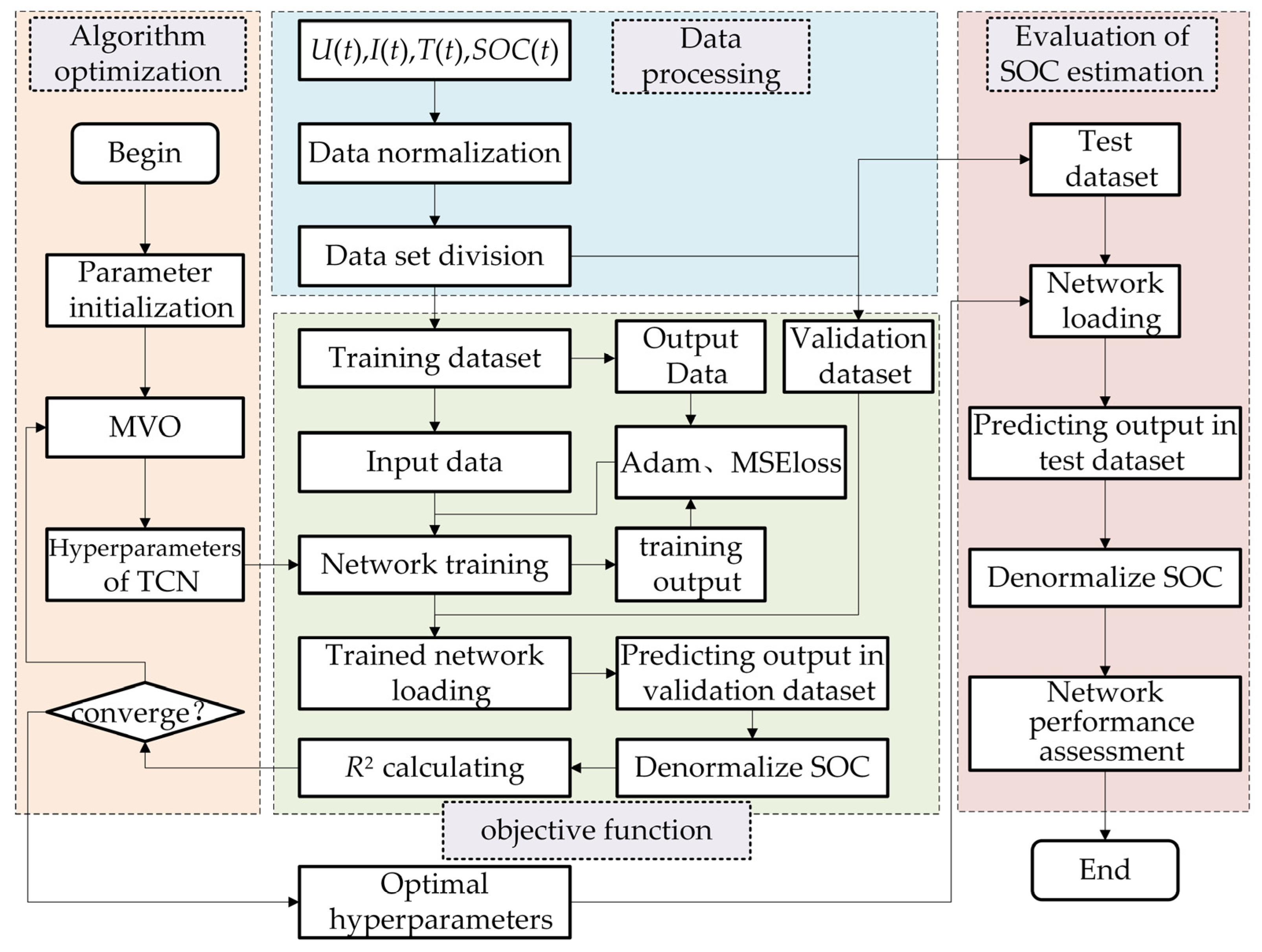
Figure 1 is the flowchart depicting the SOC estimation framework based on TCN-MVO. It is structured into four modules: data processing, algorithm optimization, objective function, and evaluation of the SOC estimation.

Figure 1. Flowchart depicting the SOC estimation framework based on TCN-MVO.

Data processing includes the techniques of data normalization and the division of datasets. The MVO algorithm is employed for optimizing the optimal hyperparameter solution of the TCN in algorithmic optimization. The objective function mainly implements the training and verification processes of deep learning. The network training uses the Adam optimizer, the loss function uses mean square error (MSE) loss, and the network verification uses the indicator R² of Equation (4) for evaluation. The closer R² is to 1, the more optimal its hyperparameters are, indicating superior performance of the training network. Finally, the optimized TCN is employed for SOC estimation, and the metrics are subsequently computed and evaluated using Equations (1)–(3).

2.3. TCN Modeling for SOC Estimation

The TCN can effectively mitigate common deficiencies in recurrent neural networks, such as gradient vanishing and exploding. Through parallel computation, the network’s performance can be enhanced. The SOC estimation will be performed utilizing the TCN in this work.

Figure 2 illustrates the basic architecture of the TCN. It is apparent that the TCN model is primarily constructed through the interconnection of residual blocks. These blocks comprise causal convolutions, dilated convolutions, weight normalization, rectified linear unit (ReLU) activation function, random dropout, and 1 × 1 convolution. The incorporation of a 1 × 1 convolution facilitates the transfer of network information across layers while maintaining consistency in input–output dimensions. The symbol “*” following ReLU indicates its presence in all layers except the final one, ensuring the potential for negative output values.

Figure 2. Basic architecture diagram of the TCN.

Figure 3 depicts a schematic of dilated causal convolution. Causal convolution is unidirectional, implying that the data in layer i at time k only depend on the data at or before time k in layer i − 1. The augmentation of network layers holds the potential to enhance the capabilities of acquiring long-range data. Dilated convolution refers to the insertion of gaps or holes within the conventional convolution operation, where the sampling rate is regulated by a dilation factor denoted as d. It achieves an increased receptive field by employing spaced sampling. With a larger dilation factor d, the convolutional output can capture information from longer temporal sequences without compromising information integrity. This method allows for a larger receptive field with fewer network layers. Meanwhile, n refers to the number of residual blocks, and b denotes the dilation base. It follows that d can be calculated as d = b⁽ⁿ⁻¹⁾. Zero-padding is necessary for each layer of the network due to the incorporation of holes in dilated convolutions. The padding amount p is determined by the convolution kernel size k_s and satisfies the condition k_s ≥ b, where p = (k_s − 1) · d.

Figure 3. Schematic diagram of dilated causal convolution.

As a residual block is composed of two causal convolution layers, the total receptive field size, denoted as r_f, for the TCN is given by:

$$r_{\mathrm{f}}=1+\sum _{i=0}^{n-1}2\cdot (k_{\mathrm{s}}-1)\cdot b^i=1+2\cdot (k_{\mathrm{s}}-1)\cdot \frac{b^n-1}{b-1}.$$

(5)

The minimum number of residual blocks required to fully cover the input sequence is given by:

$$n=⌈{\log }_b\left(\frac{(l-1)\cdot (b-1)}{(k_{\mathrm{s}}-1)\cdot 2}+1\right)⌉$$

(6)

where l denotes the length of the input sequence, and ⌈x⌉ represents rounding x up to the nearest integer. Computing this value ensures that the TCN is sufficiently deep to cover all the information in the input sequence.

The network employs a sliding window method to process the input data. Figure 4 presents the input and output data format schematic for the SOC estimation method. At time k, the vector $\chi (k)$ = [U(k), I(k), T(k)]^T denotes a vector consisting of the terminal voltage, current, and surface temperature of the battery, with $\gamma (k)$ indicating a vector of the estimated SOC.

Figure 4. Input and output data format schematic for the SOC estimation method.

Additionally, the min–max normalization method is employed for data normalization, aiming to enhance the training adaptability of deep learning networks, alleviate neuron saturation, and improve algorithmic estimation accuracy. The formula for min–max normalization is:

$$\begin{gathered} x’(k)=\left[x(k)-x_{\min }\right]/(x_{\max }-x_{\min }), \\ y’(k)=\left[y(k)-y_{\min }\right]/(y_{\max }-y_{\min }). \end{gathered}$$

(7)

At time k, the network’s overall input and output are mathematically expressed as:

$$\begin{gathered} \chi (k)=[x\prime (k-L_{\mathrm{window}}+1),x\prime (k-L_{\mathrm{window}}+2),\dots ,x\prime (k)], \\ \gamma (k)=y\prime (k), \end{gathered}$$

(8)

where L_window denotes the window size of the input data.

After obtaining the network’s predicted output value, denoted as $\widehat{y}\prime (k)$, the inverse normalization is performed, and the estimated SOC is given by:

$$SOC(k)=\widehat{y}\prime (k)\cdot (y_{\max }-y_{\min })+y_{\min }$$

(9)

Moreover, the network training will employ the MSE loss function. Given a total of n training data samples, the loss function can be represented as follows:

$$L_{\mathrm{MSE}}=\frac{1}{n}\sum _{i=1}^n{\left(y\prime {(k)}_i-\widehat{y}\prime {(k)}_i\right)}^2$$

(10)

2.4. MVO Method for Optimization of TCN Hyperparameters

Mirjalili et al. [39] proposed a multi-verse optimizer derived from the principles of the multiverse theory. This algorithm simulates the transfer of objects through white-hole/black-hole tunnels to search for the best solution. The MVO algorithm comprises exploration and exploitation phases, where white holes repel objects during higher cosmic expansion rates, while black holes attract and absorb objects during lower rates. The algorithm introduces “white hole/black hole tunnels” connecting universes for object transfer. In the exploitation phase, wormholes connect universes to the optimal one, allowing for potential object transfer. Wormhole generation probability is independent of the cosmic expansion rate. The algorithm leverages the trend of objects from high to low inflation rates in the random generation process, facilitating object migration and progressive exploration of the search space toward optimal positions based on cosmological principles.

Figure 5 depicts the schematic diagram of the MVO algorithm. The inflation rate of the n^th universe is represented by I(U_n), as shown in Figure 5, where I(U₁) > I(U₂) > … > I(U_n). In the establishment of tunnels connecting two universes, a universe characterized by a higher inflation rate is more inclined to accommodate a white hole, whereas a universe with a lower inflation rate is more likely to host a black hole. The transfer of objects from a universe with a high inflation rate to one with a low inflation rate is highly likely, thereby contributing to the overall average inflation rate of the universe during successive iterations.

Figure 5. Schematic diagram of the MVO algorithm.

As depicted in Figure 5, the objects are symbolized by the white dots that are transported via wormholes. The generation of these wormholes does not take into account the inflation rate of the universe, thereby presenting optimization opportunities for each individual universe. The utilization of wormholes is exclusively limited to connecting the currently optimal individual universes in order to achieve optimization in the search space. By employing white hole/black hole tunnels and wormholes, the MVO algorithm facilitates the continuous transfer of objects between other universes and the current optimal universe, thereby iterating toward optimization. In this process, individuals in each universe symbolize feasible solutions to the optimization problem, where objects in the universe denote design variables, and the inflation rate of the universe acts as the fitness value for the objective function.

Figure 6 illustrates the flowchart of the MVO algorithm, where U represents the randomly initialized universes, d denotes the number of design variables, and N_p signifies the population size. In the exploration phase, mathematical modeling is employed to study the inter-universe exchange of objects through white-/black-hole tunnels. The algorithm incorporates a roulette wheel selection mechanism, where universes are ranked based on their inflation rates in each iteration, and a universe containing a white hole is chosen using this selection method. Let $x_i^j$ denote the j^th design variable in the i^th universe, where U_i denotes the i^th universe and NI(i) indicates its normalized inflation rate. Let r₁ be a uniformly distributed random number between 0 and 1, and let $x_k^j$ represent the j^th design variable in the k^th universe selected through a roulette wheel mechanism. $x_i^j$ is given by:

$$x_i^j=\left\{\begin{array}{c}{x}_k^j\hspace{1em}r1<NI(U_i)\\ x_i^j\hspace{1em}r1\ge NI(U_i)\end{array}\right..$$

(11)

Figure 6. Flowchart of the MVO algorithm.

During the exploitation phase, any universe has the potential to generate a wormhole, thereby establishing a connection with the currently optimal universe and facilitating the exchange of objects. Let $X_j$ denote the current optimal value of the j^th design variable, l_tdr represent the rate of travel distance, p_wep be the probability of wormhole existence in the universe, and u_bj and l_bj indicate the upper and lower bounds for the j^th design variable. Additionally, r₂, r₃, and r₄ are random numbers within the range [0, 1]. $x_i^j$ is updated by:

$$x_i^j=\left\{\begin{array}{l}\left\{\begin{array}{l}{X}_j+l_{\mathrm{tdr}}\cdot ((u{b}_j-l{b}_j)\cdot r_4+l{b}_j)\hspace{1em}{r}_3<0.5\\ X_j-l_{\mathrm{tdr}}\cdot ((u{b}_j-l{b}_j)\cdot r_4+l{b}_j)\hspace{1em}{r}_3\ge 0.5\end{array}\right.\hspace{1em}{r}_2<p_{\mathrm{wep}}\\ x_i^j\hspace{1em}\hspace{1em}\hspace{1em}\hspace{1em}\hspace{1em}\hspace{1em}\hspace{1em}\hspace{1em}\hspace{1em}\hspace{1em}\hspace{1em}\hspace{1em}\hspace{1em}\hspace{1em}\hspace{1em}\hspace{1em}{r}_2\ge p_{\mathrm{wep}}\end{array}\right..$$

(12)

The current iteration number is denoted as N_c, the maximum iteration number as N_epoch, and p_{wep_min} and p_{wep_max} denote the minimum and maximum values of p_wep, respectively. Additionally, p represents the exploitation rate. p_wep and l_tdr are given by:

$$\left\{\begin{array}{l}{p}_{\mathrm{wep}}=p_{\mathrm{wep},\min }+N_{\mathrm{c}}\cdot (p_{\mathrm{wep},\max }-p_{\mathrm{wep},\min })/N_{\mathrm{epoch}}\\ l_{\mathrm{tdr}}=1-N_{\mathrm{c}}{}^{1/p}/N_{\mathrm{epoch}}{}^{1/p}\end{array}\right..$$

(13)

2.5. Objective Function

The objective function is of paramount importance in optimizing deep learning networks through MVO. In this investigation, the design variables represent the hyperparameters of the deep learning network, and the output is indicated by −R² on the validation set. The objective function subjected to optimization in the MVO process for deep learning networks cannot be directly expressed through a mathematical equation. To construct the objective function, we present the pseudocode outlined in Table 1, which delineates the process. Steps 1 to 4 involve data preprocessing; Step 5 pertains to network model construction; Steps 6 to 12 encompass network training; and Steps 13 to 17 cover the calculation of the objective function value.

Table 1. Pseudo-code description of the objective function.

Step	Description
1:	Allocate each element of input x to respective hyperparameters and convert to required types
2:	Load training and validation set data
3:	Normalize data
4:	Convert data to tensor format and create data iterators
5:	Build deep learning network model
6:	Network Training:
7:	for i in [1: training epochs]
8:	Train network on training set and save weights
9:	Validate network on validation set and calculate R2
10:	End
11:	Compare the R2 values of all networks, and select and record the weights of the network that performs best (highest R2) on the validation set.
12:	Remove weights of non-best-performing networks
13:	End
14:	Load weights of the currently best-performing network
15:	Use the deep learning model to predict SOC on the validation set
16:	Denormalize the estimated SOC
17:	Calculate and return −R2

3. Results and Discussion

In this study, three distinct deep learning networks, including LSTM, Transformer, and TCN, are employed for estimating the SOC, and their respective performances are thoroughly compared. During the training process, the number of training epochs was set to 150, with a training batch size of 128. The deep learning networks in this section were implemented using the Pytorch framework and trained on an NVIDIA GeForce RTX 3090 (24 GB) GPU running Windows 10 (64-bit) with Python 3.8.

The hyperparameters subject to optimization for various deep learning networks are as follows: (1) LSTM: Sliding window length ($L_{\mathrm{win}\_\mathrm{size}}^{\mathrm{lstm}}$), Hidden layer output dimension ($N_{\mathrm{hidden}\_\mathrm{size}}^{\mathrm{lstm}}$), Fully connected layer output dimension ($N_{\mathrm{out}}^{\mathrm{lstm}}$), Random dropout rate ($d_{\mathrm{r}}^{\mathrm{lstm}}$), Learning rate ($l_{\mathrm{r}}^{\mathrm{lstm}}$). (2) Transformer: Sliding window length ($L_{\mathrm{win}\_\mathrm{size}}^{\mathrm{trans}}$), Number of attention heads ($N_{\mathrm{head}}^{\mathrm{trans}}$), Embedding dimension ($N_{\mathrm{embed}}^{\mathrm{trans}}$), Feedforward network dimension ($N_{\mathrm{forward}}^{\mathrm{trans}}$), Number of encoder layers ($N_{\mathrm{layer}}^{\mathrm{trans}}$), Random dropout rate ($d_{\mathrm{r}}^{\mathrm{trans}}$), Learning rate ($l_{\mathrm{r}}^{\mathrm{trans}}$). (3) TCN: Sliding window length ($L_{\mathrm{win}\_\mathrm{size}}^{\mathrm{tcn}}$), Number of hidden layer channels ($N_{\mathrm{ch}1}^{\mathrm{tcn}}$, $N_{\mathrm{ch}2}^{\mathrm{tcn}}$, $N_{\mathrm{ch}3}^{\mathrm{tcn}}$), Convolutional kernel size ($k_{\mathrm{s}}^{\mathrm{tcn}}$), Random dropout rate ($d_{\mathrm{r}}^{\mathrm{tcn}}$), and Learning rate ($l_{\mathrm{r}}^{\mathrm{tcn}}$).

3.1. Dataset

A publicly accessible dataset graciously provided by the University of Wisconsin-Madison [40] was utilized to estimate the SOC for the Panasonic 18650PF battery with a nominal voltage of 3.6 V. The dataset includes nine operating conditions, covering four fundamental scenarios: aggressive driving (SFTP-US06), high-speed (HWFET), urban road cycling (UDDS), and LA92. Additionally, five mixed conditions—Cycles 1 to 4 and a neural network (NN) condition—are included. Cycles 1 to 4 are randomly formed from US06, HWFET, UDDS, LA92, and NN conditions. The NN condition intricately blends segments of the US06 and LA92 driving cycles, introducing supplementary dynamics beneficial for neural network training. This comprehensive method aims to reveal the comparative performance of LSTM, Transformer, and TCN under diverse real-world conditions.

The NN condition, intentionally designed to encompass dynamic scenarios that are beneficial for neural network training within the dataset, was consistently utilized for training in all subsequent design examples. Training, optimization, and testing were conducted at both fixed and varied ambient temperatures. To facilitate a comprehensive comparison of different deep learning networks, two distinct dataset splitting methods were employed:

(A) The training set includes basic scenarios (US06 + UDDS + LA92 + HWFET) along with the NN condition; the validation set includes mixed scenarios (Cycle 1 + Cycle 2); and the testing set includes mixed scenarios (Cycle 3 + Cycle 4).

(B) The training set includes mixed scenarios (Cycle 1~4 + NN); the validation set includes basic scenarios (LA92 + HWFET); and the testing set includes basic scenarios (US06 + UDDS).

3.2. Network Training and Testing at a Fixed Ambient Temperature

This section begins by describing the preliminary tests to evaluate the SOC estimation capabilities of different networks, namely, LSTM, Transformer, and TCN. The focus is on examining their mapping abilities for the nonlinear relationships between LIB voltage, current, surface temperature, and SOC at a fixed ambient temperature of 25 °C. The deep learning networks undergo training, optimization, and testing specifically at this fixed temperature.

The MVO algorithm was employed to optimize the hyperparameters for LSTM, Transformer, and TCN at a fixed temperature of 25 °C using two distinct dataset splitting methods. After optimization using the MVO algorithm, the R² values for the validation datasets, obtained through two distinct dataset splitting methods, were very close to 1, indicating the convergence of the algorithm. Furthermore, this signifies a robust fit to the validation set, reflecting a high level of model fitting. Table 2 presents the optimization results of the hyperparameters for different networks using the MVO algorithm at a fixed temperature of 25 °C. Table 3 presents the evaluation metrics results for the test dataset at a fixed temperature of 25 °C. Observations suggest that in dataset splitting method A, the RMSE and MAE for all three networks remained below 1%, with the TCN exhibiting the smallest values for both, measuring 0.6959% and 0.4945%, respectively. The TCN’s MAX, although positioned in the middle among these three methods, exhibited a mere 0.5604% deviation from the lowest MAX observed with LSTM. In dataset splitting method B, the TCN achieved the lowest RMSE, MAE, and MAX, with only the TCN’s RMSE being below 1%, measuring 0.9160%. Additionally, its MAE and MAX were recorded at 0.7937% and 2.8759%, respectively. These results validate that at a constant ambient temperature, the proposed MVO-TCN method surpasses the other two methods in achieving optimal performance in SOC estimation.

Table 2. Optimization results of the hyperparameters for different networks using the MVO algorithm at a fixed temperature of 25 °C.

Network	Result for dataset splitting method A
LSTM	$L_{\mathrm{win}\_\mathrm{size}}^{\mathrm{lstm}}$	$N_{\mathrm{hidden}\_\mathrm{size}}^{\mathrm{lstm}}$	$N_{\mathrm{out}}^{\mathrm{lstm}}$	$d_{\mathrm{r}}^{\mathrm{lstm}}$	$l_{\mathrm{r}}^{\mathrm{lstm}}$
	73	143	121	0	5.3129 × 10−3
Transformer	$L_{\mathrm{win}\_\mathrm{size}}^{\mathrm{trans}}$	$N_{\mathrm{head}}^{\mathrm{trans}}$	$N_{\mathrm{embed}}^{\mathrm{trans}}$	$N_{\mathrm{forward}}^{\mathrm{trans}}$	$N_{\mathrm{layer}}^{\mathrm{trans}}$	$d_{\mathrm{r}}^{\mathrm{trans}}$	$l_{\mathrm{r}}^{\mathrm{trans}}$
	65	4	44	124	1	0.0178	7.4701 × 10−3
TCN	$L_{\mathrm{win}\_\mathrm{size}}^{\mathrm{tcn}}$	$N_{\mathrm{ch}1}^{\mathrm{tcn}}$	$N_{\mathrm{ch}2}^{\mathrm{tcn}}$	$N_{\mathrm{ch}3}^{\mathrm{tcn}}$	$k_{\mathrm{s}}^{\mathrm{tcn}}$	$d_{\mathrm{r}}^{\mathrm{tcn}}$	$l_{\mathrm{r}}^{\mathrm{tcn}}$
	92	96	120	52	10	0.0488	2.5526 × 10−3
Network	Result for dataset splitting method B
LSTM	$L_{\mathrm{win}\_\mathrm{size}}^{\mathrm{lstm}}$	$N_{\mathrm{hidden}\_\mathrm{size}}^{\mathrm{lstm}}$	$N_{\mathrm{out}}^{\mathrm{lstm}}$	$d_{\mathrm{r}}^{\mathrm{lstm}}$	$l_{\mathrm{r}}^{\mathrm{lstm}}$
	96	100	122	0.0186	3.2398 × 10−3
Transformer	$L_{\mathrm{win}\_\mathrm{size}}^{\mathrm{trans}}$	$N_{\mathrm{head}}^{\mathrm{trans}}$	$N_{\mathrm{embed}}^{\mathrm{trans}}$	$N_{\mathrm{forward}}^{\mathrm{trans}}$	$N_{\mathrm{layer}}^{\mathrm{trans}}$	$d_{\mathrm{r}}^{\mathrm{trans}}$	$l_{\mathrm{r}}^{\mathrm{trans}}$
	99	4	44	149	4	0	7.3799 × 10−4
TCN	$L_{\mathrm{win}\_\mathrm{size}}^{\mathrm{tcn}}$	$N_{\mathrm{ch}1}^{\mathrm{tcn}}$	$N_{\mathrm{ch}2}^{\mathrm{tcn}}$	$N_{\mathrm{ch}3}^{\mathrm{tcn}}$	$k_{\mathrm{s}}^{\mathrm{tcn}}$	$d_{\mathrm{r}}^{\mathrm{tcn}}$	$l_{\mathrm{r}}^{\mathrm{tcn}}$
	96	177	110	114	8	0	4.5545 × 10−3

Table 3. Evaluation metrics results for the test dataset at the fixed temperature of 25 °C.

Network	Dataset Splitting Method A				Dataset Splitting Method B
	RMSE (%)	MAE (%)	MAX (%)	R2	RMSE (%)	MAE (%)	MAX (%)	R2
LSTM	0.7814	0.5178	4.0052	0.9996	1.1654	0.9620	3.3061	0.9995
Transformer	0.7730	0.6046	4.6585	0.9994	1.0849	0.9693	5.2219	0.9995
TCN	0.6959	0.4945	4.5656	0.9996	0.9160	0.7937	2.8759	0.9995

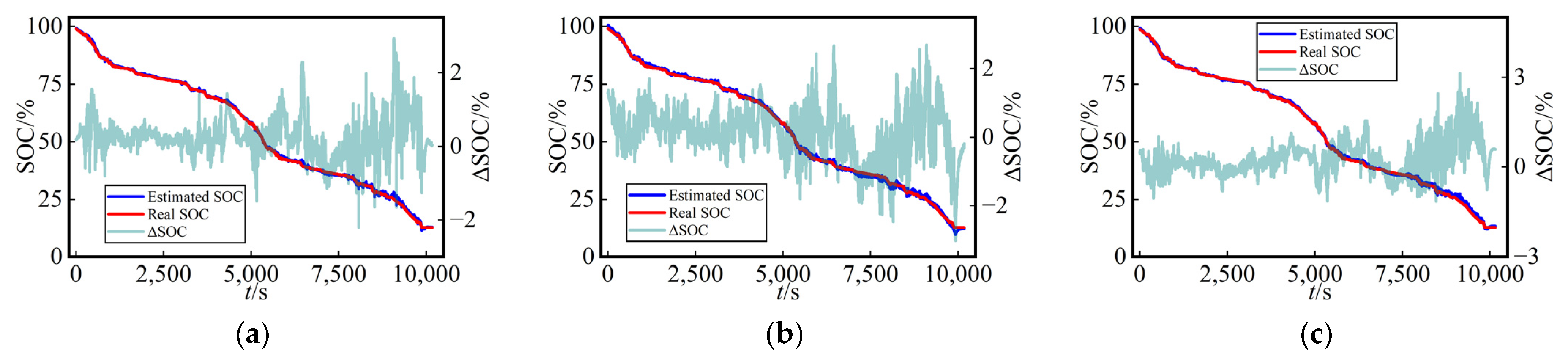
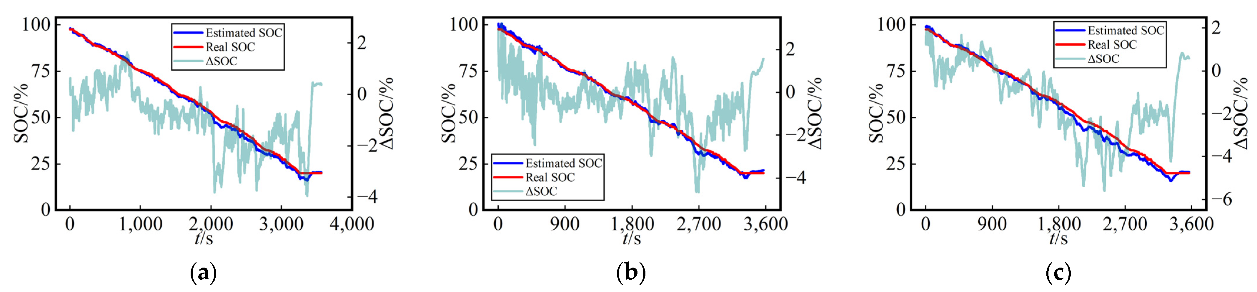
For a more straightforward assessment of the SOC estimation performance among the three methods in the test dataset, Figure 7 presents the curves of SOC estimation values and their errors (ΔSOC, calculated as the estimated value minus the true value) for the test dataset using three different networks at a fixed temperature (25 °C) with various dataset split methods. The SOC estimation curves and true SOC curves demonstrated a remarkably high level of consistency for the three methods employed, providing compelling evidence for the viability of this work.

Figure 7. Curves of SOC estimation values and their errors for the test dataset using three different networks at a fixed temperature (25 °C) with various dataset split methods: (a) LSTM, (b) Transformer, (c) TCN at Cycle 3 with dataset split method A; (d) LSTM, (e) Transformer, (f) TCN at Cycle 4 with dataset split method A; (g) LSTM, (h) Transformer, (i) TCN at US06 with dataset split method B; (j) LSTM, (k) Transformer, (l) TCN at UDDS with dataset split method B.

3.3. Network Training and Testing at Various Ambient Temperatures

To further compare the mapping capabilities of the three distinct deep learning networks for characterizing the nonlinear dependencies among voltage, current, surface temperature, and SOC in lithium-ion batteries, simultaneous training, optimization, and testing were conducted at various ambient temperatures (0 °C, 10 °C, and 25 °C). Because the dataset covers various operating conditions at multiple ambient temperatures, the nonlinear relationship among the voltage, current, surface temperature, and SOC becomes more complex. This complexity necessitates a more comprehensive evaluation of the different deep learning networks’ performances. The performances of these three methods were compared using both aforementioned dataset splitting methods at various ambient temperatures.

3.3.1. Network Training and Testing Using the Dataset Splitting Method A

The MVO algorithm was adopted to optimize the hyperparameters for three networks, namely, LSTM, Transformer, and TCN, using dataset splitting method A. The dataset encompasses nine dynamic operating conditions across various ambient temperatures. Table 4 presents the optimization results of the hyperparameters for the different networks using the MVO algorithm at various ambient temperatures (0 °C, 10 °C, and 25 °C) using dataset splitting method A. After optimization using the MVO algorithm, the R² values for the validation dataset (Cycle1 + Cycle2) were close to 1 across all three deep learning networks, indicating that the MVO algorithm effectively converged. Additionally, the results reveal that all three networks demonstrate exceptional fitting of the intricate relationships among voltage, current, surface temperature, and SOC for the validation dataset through the data from diverse dynamic working conditions at various temperatures.

Table 4. Optimization results of hyperparameters for different networks using the MVO algorithm at various ambient temperatures (0 °C, 10 °C, and 25 °C) with dataset splitting method A.

Network	Result
LSTM	$L_{\mathrm{win}\_\mathrm{size}}^{\mathrm{lstm}}$	$N_{\mathrm{hidden}\_\mathrm{size}}^{\mathrm{lstm}}$	$N_{\mathrm{out}}^{\mathrm{lstm}}$	$d_{\mathrm{r}}^{\mathrm{lstm}}$	$l_{\mathrm{r}}^{\mathrm{lstm}}$
	73	196	166	0.1037	1.0449 × 10−3
Transformer	$L_{\mathrm{win}\_\mathrm{size}}^{\mathrm{trans}}$	$N_{\mathrm{head}}^{\mathrm{trans}}$	$N_{\mathrm{embed}}^{\mathrm{trans}}$	$N_{\mathrm{forward}}^{\mathrm{trans}}$	$N_{\mathrm{layer}}^{\mathrm{trans}}$	$d_{\mathrm{r}}^{\mathrm{trans}}$	$l_{\mathrm{r}}^{\mathrm{trans}}$
	75	2	124	198	3	0.0767	1 × 10−4
TCN	$L_{\mathrm{win}\_\mathrm{size}}^{\mathrm{tcn}}$	$N_{\mathrm{ch}1}^{\mathrm{tcn}}$	$N_{\mathrm{ch}2}^{\mathrm{tcn}}$	$N_{\mathrm{ch}3}^{\mathrm{tcn}}$	$k_{\mathrm{s}}^{\mathrm{tcn}}$	$d_{\mathrm{r}}^{\mathrm{tcn}}$
	76	105	53	50	9	0.1197	1.2022 × 10−3

Table 5 presents the evaluation metrics results for the test dataset (Cycle 3+ Cycle 4) at various ambient temperatures (0 °C, 10 °C, and 25 °C) using dataset splitting method A. The RMSE and MAE values below 1% were obtained for the SOC estimation on the test dataset across all three methods. Notably, the proposed MVO-TCN achieved the smallest RMSE and MAE, measuring 0.6790% and 0.4904%, respectively. Among these methods, the TCN exhibited a moderate MAX value of SOC estimation at 4.2517%, but it was only 0.3944% larger than the lowest MAX observed with Transformer. In summary, the proposed MVO-TCN demonstrates the optimal performance in SOC estimation among the three methods considered in this study.

Table 5. Evaluation metrics results for the test dataset (Cycle 3 + Cycle 4) at various ambient temperatures (0 °C, 10 °C, and 25 °C) with dataset splitting method A.

Network	RMSE (%)	MAE (%)	MAX (%)	R2
LSTM	0.7766	0.5752	5.6381	0.9989
Transformer	0.7388	0.5806	3.8573	0.9991
TCN	0.6790	0.4904	4.2517	0.9991

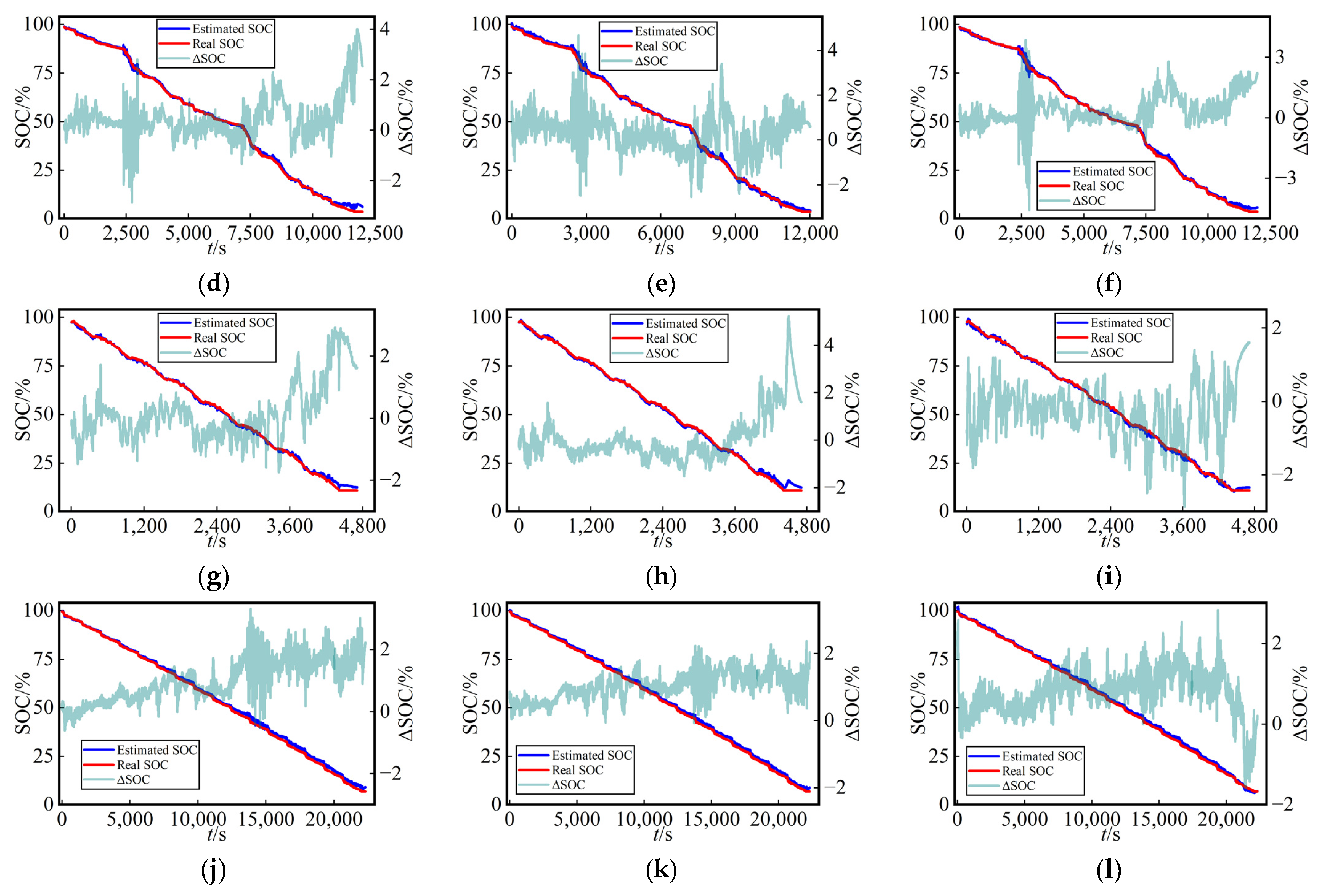
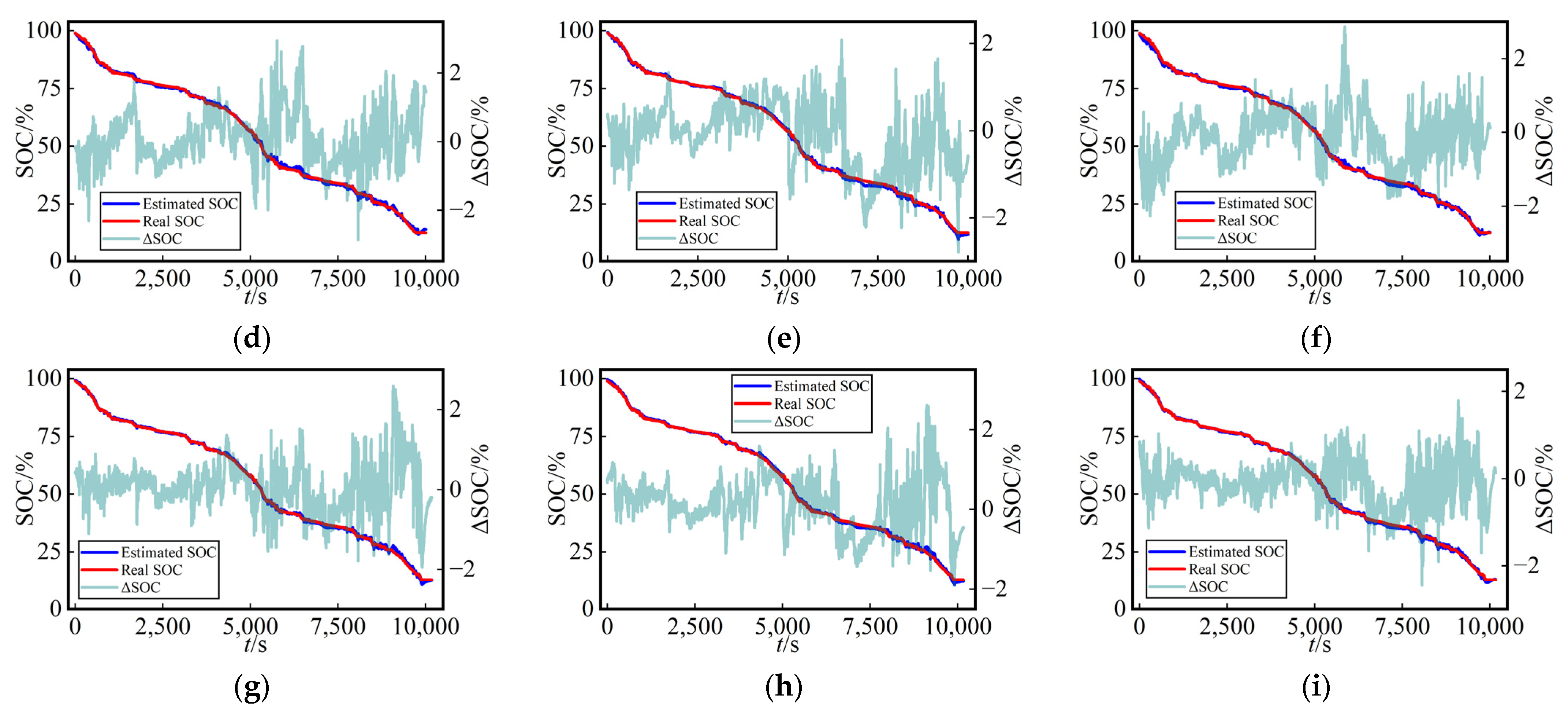
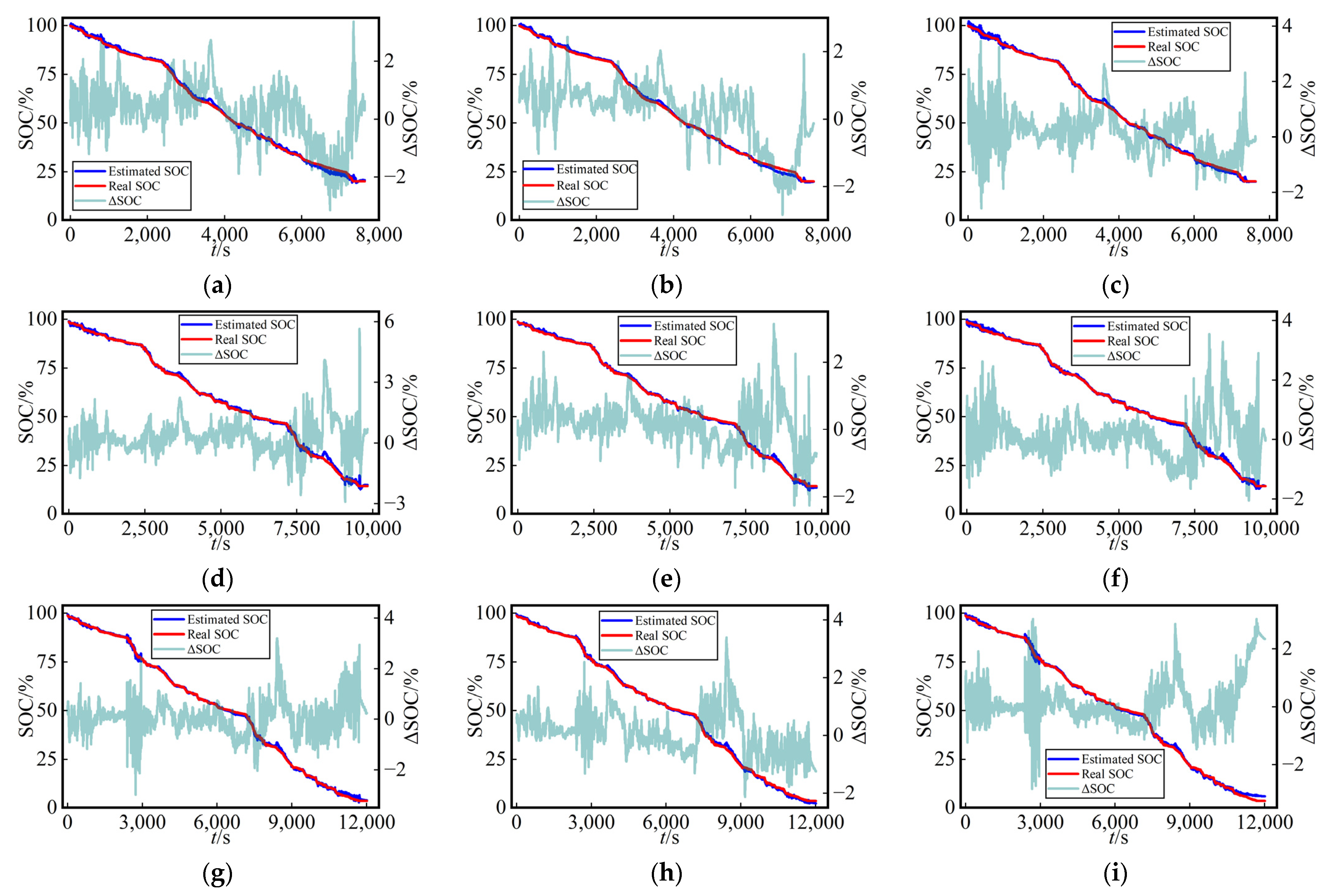
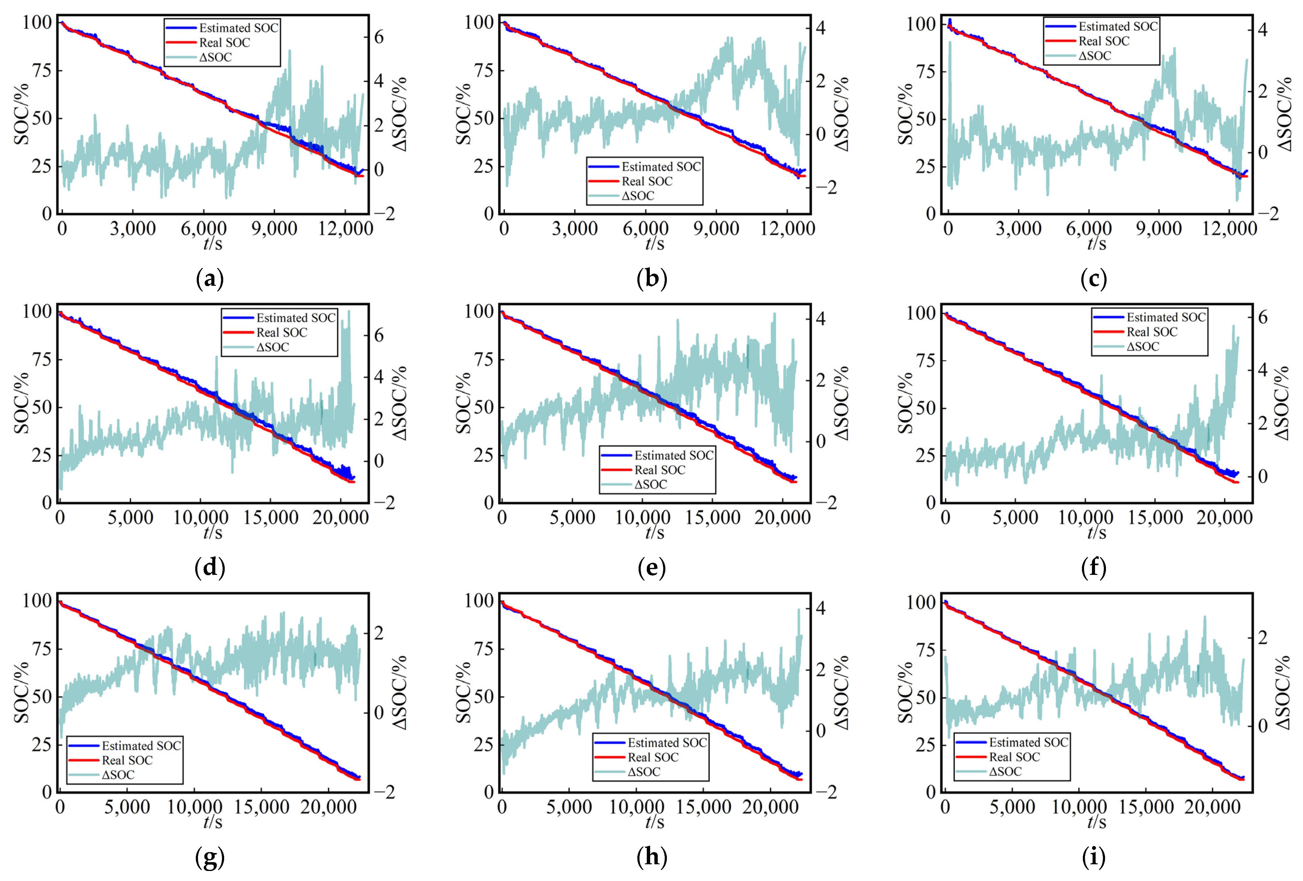
Similarly, for a comparison that is more easily interpretable in terms of the battery’s SOC estimation at various ambient temperatures in the test dataset, as depicted in Figure 8 and Figure 9, the following figure presents the curves of estimated SOC values, actual values, and their errors (ΔSOC, calculated as the estimated value minus the true value) for the three networks at different ambient temperatures in test Cycles 3 and 4. The three methods yielded accuracy curves representing the estimated SOC. The error curves directly reflected the SOC estimation performance for different networks under various working conditions.

Figure 8. Curves of SOC estimation values and their errors for Cycle 3 in the test dataset using three different networks at various temperatures (0 °C, 10 °C, and 25 °C) with dataset split method A: (a) LSTM, (b) Transformer, and (c) TCN at 0 °C; (d) LSTM, (e) Transformer, and (f) TCN at 10 °C; (g) LSTM, (h) Transformer, and (i) TCN at 25 °C.

Figure 9. Curves of SOC estimation values and their errors for Cycle 4 in the test dataset using three different networks at various temperatures (0 °C, 10 °C, and 25 °C) with dataset split method A: (a) LSTM, (b) Transformer, and (c) TCN at 0 °C; (d) LSTM, (e) Transformer, and (f) TCN at 10 °C; (g) LSTM, (h) Transformer, and (i) TCN at 25 °C.

3.3.2. Network Training and Testing Using Dataset Splitting Method B

To study the robustness of the proposed method, we conducted training, optimization, and testing under various working conditions at various temperatures using dataset splitting method B. Table 6 presents the optimization results of the hyperparameters for different networks using the MVO algorithm at various ambient temperatures (0 °C, 10 °C, and 25 °C) using dataset splitting method B. After optimization with the MVO algorithm, the R² values for all three methods on the validation dataset (LA92 + HWFET) were also very close to 1. This suggests that MVO converged, and all three methods exhibit a good fit for the SOC estimation on the validation dataset.

Table 6. Optimization results of the hyperparameters for different networks using the MVO algorithm at various ambient temperatures (0 °C, 10 °C, and 25 °C) with dataset splitting method B.

Network	Result
LSTM	$L_{\mathrm{win}\_\mathrm{size}}^{\mathrm{lstm}}$	$N_{\mathrm{hidden}\_\mathrm{size}}^{\mathrm{lstm}}$	$N_{\mathrm{out}}^{\mathrm{lstm}}$	$d_{\mathrm{r}}^{\mathrm{lstm}}$	$l_{\mathrm{r}}^{\mathrm{lstm}}$	-	-
	97	180	181	0	4.3920 × 10−3	-	-
Transformer	$L_{\mathrm{win}\_\mathrm{size}}^{\mathrm{trans}}$	$N_{\mathrm{head}}^{\mathrm{trans}}$	$N_{\mathrm{embed}}^{\mathrm{trans}}$	$N_{\mathrm{forward}}^{\mathrm{trans}}$	$N_{\mathrm{layer}}^{\mathrm{trans}}$	$d_{\mathrm{r}}^{\mathrm{trans}}$	$l_{\mathrm{r}}^{\mathrm{trans}}$
	94	4	12	43	1	0.0009	5.1923 × 10−3
TCN	$L_{\mathrm{win}\_\mathrm{size}}^{\mathrm{tcn}}$	$N_{\mathrm{ch}1}^{\mathrm{tcn}}$	$N_{\mathrm{ch}2}^{\mathrm{tcn}}$	$N_{\mathrm{ch}3}^{\mathrm{tcn}}$	$k_{\mathrm{s}}^{\mathrm{tcn}}$	$d_{\mathrm{r}}^{\mathrm{tcn}}$	$l_{\mathrm{r}}^{\mathrm{tcn}}$
	100	120	151	151	8	0	1 × 10−4

As depicted in Table 7, among the three methods using splitting method B, the proposed MVO-TCN in this study consistently exhibited the smallest RMSE and MAE for SOC estimation across various temperatures and working conditions for the test dataset (US06 + UDDS), measuring 1.2388% and 0.9909%, respectively. Despite having a moderate MAX, it was only 1.0222% larger than the smallest MAX observed with Transformer. Overall, compared with the other two methods, this method exhibits the most optimal performance in SOC estimation.

Table 7. Evaluation metrics results for the test dataset (US06 + UDDS) at various ambient temperatures (0 °C, 10 °C, and 25 °C) with dataset splitting method A.

Network	RMSE (%)	MAE (%)	MAX (%)	R2
LSTM	1.5005	1.2642	7.1627	0.9993
Transformer	1.4205	1.1979	4.6569	0.9992
TCN	1.2388	0.9909	5.6791	0.9992

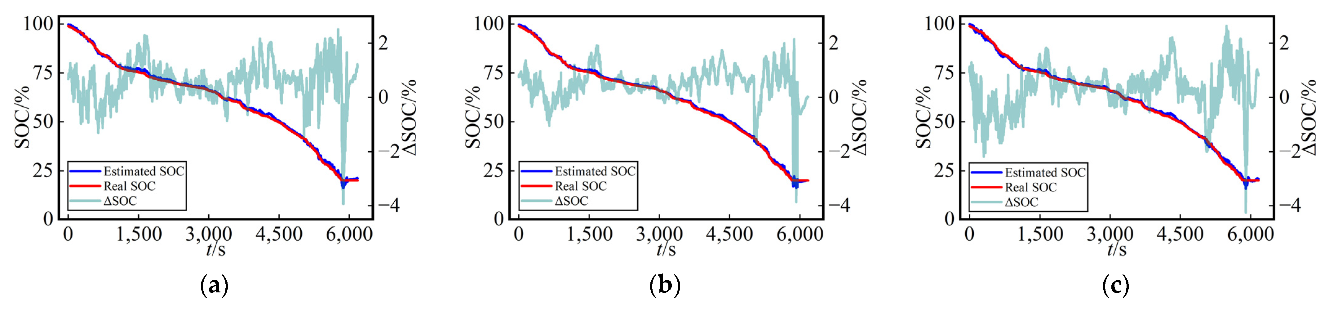
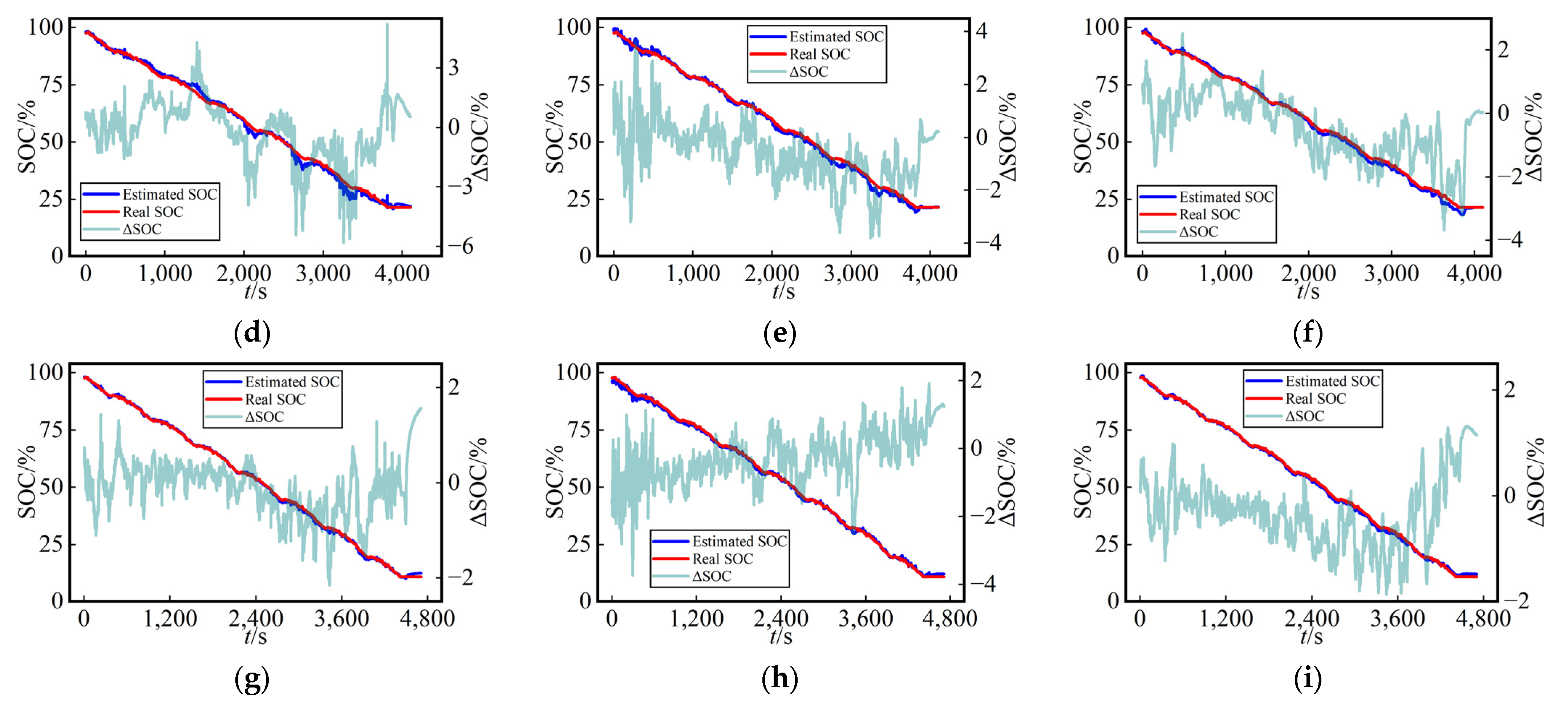
As depicted in Figure 10 and Figure 11, we noted that the estimated SOC curves and true SOC curves were nearly identical, indicating that all three networks exhibited high precision in the SOC estimation using dataset splitting method A. Additionally, the figures provide a visual representation of the error variations for each network across different temperatures and working conditions. This suggests that the proposed MVO-TCN algorithm in this study possesses a high level of robustness.

Figure 10. Curves of SOC estimation values and their errors for the US06 in the test dataset using three different networks at various temperatures (0 °C, 10 °C, and 25 °C) with dataset split method B: (a) LSTM, (b) Transformer, and (c) TCN at 0 °C; (d) LSTM, (e) Transformer, and (f) TCN at 10 °C; (g) LSTM, (h) Transformer, and (i) TCN at 25 °C.

Figure 11. Curves of SOC estimation values and their errors for the UDDS in the test dataset using three different networks at various temperatures (0 °C, 10 °C, and 25 °C) with dataset split method B: (a) LSTM, (b) Transformer, and (c) TCN at 0 °C; (d) LSTM, (e) Transformer, and (f) TCN at 10 °C; (g) LSTM, (h) Transformer, and (i) TCN at 25 °C.

4. Conclusions

In summary, this study introduces a novel SOC estimation method for lithium-ion batteries. The integration of the TCN with MVO exhibits high efficiency and effectiveness at optimizing the TCN’s hyperparameters to achieve better precision in SOC prediction. The comprehensive evaluation, conducted under various conditions, demonstrates the robustness and generalization capabilities of the proposed MVO-TCN framework compared to conventional LSTM and Transformer methods. The inclusion of diverse measurable parameters, such as voltage, current, and temperature, enhances the adaptability of the method across dynamic working conditions. By considering dynamic operating conditions, the proposed method accurately estimates SOC, aligning closely with the actual performance of electric vehicles. This work eliminates the need for complex electrochemical or circuit modeling. Moreover, the SOC estimation process is simplified by relying on historical measurement data. This developed method, featuring a memory-efficient TCN, shows practical applicability for battery management systems, providing valuable support for technological advancement. This work not only improves SOC accuracy but also contributes to the development of battery management and energy storage technologies.