Estimation of Citrus Maturity with Fluorescence Spectroscopy Using Deep Learning

Abstract

To produce high-quality citrus, the harvest time of citrus should be determined by considering its maturity. To evaluate citrus maturity, the Brix/acid ratio, which is the ratio of sugar content or soluble solids content to acid content, is one of the most commonly used indicators of fruit maturity. To estimate the Brix/acid ratio, fluorescence spectroscopy, which is a rapid, sensitive, and cheap technique, was adopted. Each citrus peel was extracted, and its fluorescence value was measured. Then, the fluorescent spectrum was analyzed using a convolutional neural network (CNN). In fluorescence spectroscopy, a matrix called excitation and emission matrix (EEM) can be obtained, in which each fluorescence intensity was recorded at each excitation and emission wavelength. Then, by regarding the EEM as an image, the Brix/acid ratio of juice from the flesh was estimated via performing a regression with a CNN (CNN regression). As a result, the Brix/acid ratio absolute error was estimated to be 2.48, which is considerably better than the values obtained by the other methods in previous studies. Hyperparameters, such as depth of layers, learning rate, and the number of filters used for this estimation, could be observed using Bayesian optimization, and the optimization contributed to the high accuracy.

1. Introduction

Citrus is one of the most popular and consumed fruits in the world. In Japan, the production of citrus was the second largest among all fruits in 2015 [1] and Satsuma mandarin (Citrus unshiu Marc.) was the most popular cultivar. Customers demand not only consistent availability but also increasingly higher-quality citrus [2,3]. To meet demand, first, the harvest time of citrus should be appropriately determined by considering the maturity. This is because, if the harvested citrus has a high level of maturation, it is more susceptible to mechanical damage or infections during its postharvest handling. In contrast, if it is not matured, it does not have a good appearance and flavor, and may be unmarketable [4].

As indicators of citrus maturity, color change, firmness, size, shape, and the Brix/acid ratio have been widely used [4,5,6]. Brix and acidity, especially, are important parameters that represent the sugar or soluble solids content and acid content, respectively. Their ratio, that is, the Brix/acid ratio is one of the most commonly used indicators of fruit maturity, in addition to juice quality [7]. The precise estimation of the Brix/acid ratio determines the appropriate harvest time.

Previously, the internal quality was estimated based on the external factors, including its size, shape, mass, and color. However, the Brix and acidity values could not be accurately estimated [8]. Antonucci et al. [9] estimated the Brix and acidity values with a portable visible-near infrared (VIS-NIR) spectrophotometer; however, this method is comparatively expensive. Another method, fluorescence spectroscopy, which is a rapid, sensitive, and cheap technique [10], has been recently attracting attention. Muharfiza et al. [11] investigated the potential of fluorescence spectroscopy for estimating the maturity stage of Satsuma mandarins. The fluorescence characteristics were monitored during the growth and maturation stages and compared with the standard maturity index, the Brix/acid ratio. The study observed that the fluorescence peaks of amino acid and chlorophyll were related to the Brix/acid ratio and the peak intensity was useful for estimating the Brix/acid ratio. However, the accuracy of Brix/acid ratio estimation has not been quantitatively investigated yet. Further, the study adopted only two fluorescence peaks for the estimation, although a citrus peel has various fluorescence peaks. Moreover, if information other than peaks, such as shoulder [12], unevenness, and valleys of fluorescence spectrum, are considered, the estimation accuracy would be increased [13].

Recently, convolutional neural network (CNN), which is one type of deep learning, achieved high classification accuracy in image analysis. In CNN, relevant contextual features in image categorization problems are automatically discovered; therefore, CNNs are attracting attention [14].

In fluorescence spectroscopy, an excitation and emission matrix (EEM) can be obtained, wherein each fluorescence intensity was recorded at each excitation and emission wavelength. Then, we assumed that by regarding the EEM as an image, the Brix/acid ratio can be accurately estimated with a CNN. To date, few studies have tried a CNN for EEM and estimated fruit internal quality. In the field of agricultural product and plant evaluation, CNN has recently started being used [15,16,17,18]. However, the main objective has been categorical classification and fewer studies have conducted regression with a CNN (or CNN regression [19]) to quantitatively predict quality.

A considerable problem in the use of a CNN is the adjustment of the hyperparameter. Substantial parameters, such as depth of layers, learning rate, and number of filters, should be optimized. The optimal parameters change according to the sample and the objective. It is difficult, expensive, and time-consuming to construct good architecture of a network [20,21].

Previously, to optimize the hyperparameters, grid search and random search, which try all parameters one by one and select the parameters randomly, have been utilized. However, in a grid search, it incurs a considerable cost and time to check all potential patterns. In a random search, as the number of parameters to be optimized increase, it becomes more difficult to obtain good parameters.

A good choice is Bayesian optimization [22], which has been shown to outperform other optimization algorithms. Bayesian optimization typically assumes that the unknown function was sampled from a Gaussian process. Bayesian optimization is particularly effective when it is computationally expensive to find out the optimized hyperparameters from numerous patterns [23]. Using the Bayesian optimization algorithm, it would be possible to optimize the parameters efficiently.

In this study, the hyperparameter optimization for CNN was first optimized with Bayesian optimization. With the determined parameters, CNN regression was performed for Brix/acid ratio estimation. Then, the estimated value was compared with the actual value, and the estimation accuracy was investigated.

2. Materials and Methods

2.1. Materials and Spectra Measurement

From September to December, about 15 Satsuma mandarins (cv. Miyagawa Wase) in Ehime prefecture, Japan, were harvested every month and 47 citrus fruits whose peels were not damaged were used for this experiment. After peeling, the citrus peel was extracted with chloroform as recommended by Muharfiza et al. [11]. Immediately after extraction, their fluorescence measurement was conducted with a fluorometer (FP-8300, Jasco Co., Tokyo, Japan). The scanned excitation (Ex) and emission (Em) wavelengths were observed to be between 200 to 550 nm and 210 to 750 nm, respectively. Figure 1 shows an example of an EEM for citrus peel. The brightness of the color represents the fluorescence intensity. For CNN regression, the area with the emission wavelength from 300 to 700 nm was picked. Spectra measurement was conducted three times for the same sample. The citrus flesh of each peeled fruit was squeezed by hand, and its Brix/acid ratio was measured by a hand-held digital refractometer (PAL-BX, Atago Co., Ltd., Tokyo, Japan). We confirmed the refractometer was reliable using titration. The experimental flow after sample preparation is described in Figure 2.

2.2. Estimation of the Brix/Acid Ratio with CNN Regression

In this study, one of the most general types of CNN, containing a convolution layer, a pooling layer, and a fully-connected layer, was adopted [21,24]. To perform CNN regression and estimate the Brix/acid ratio, the regression layer was put in the final layer. As a loss function [25], mean square error was defined. The weight of each filter and bias was adjusted to minimize the mean square error between the actual and estimated Brix/acid ratios and the estimated value.

A total of 141 EEM spectra, like the one shown in Figure 1, obtained from September to December were split into 121 training data and 20 test data. The input image was a 2-D image whose x and y axes corresponded to the emission and excitation wavelengths. The fluorescence intensity was recorded in the 2-D image as a pixel value. The estimation with the CNN regression as shown above was conducted five times every time, and their average value represented the estimation result. First, the hyperparameters for estimation were optimized using Bayesian optimization as explained below.

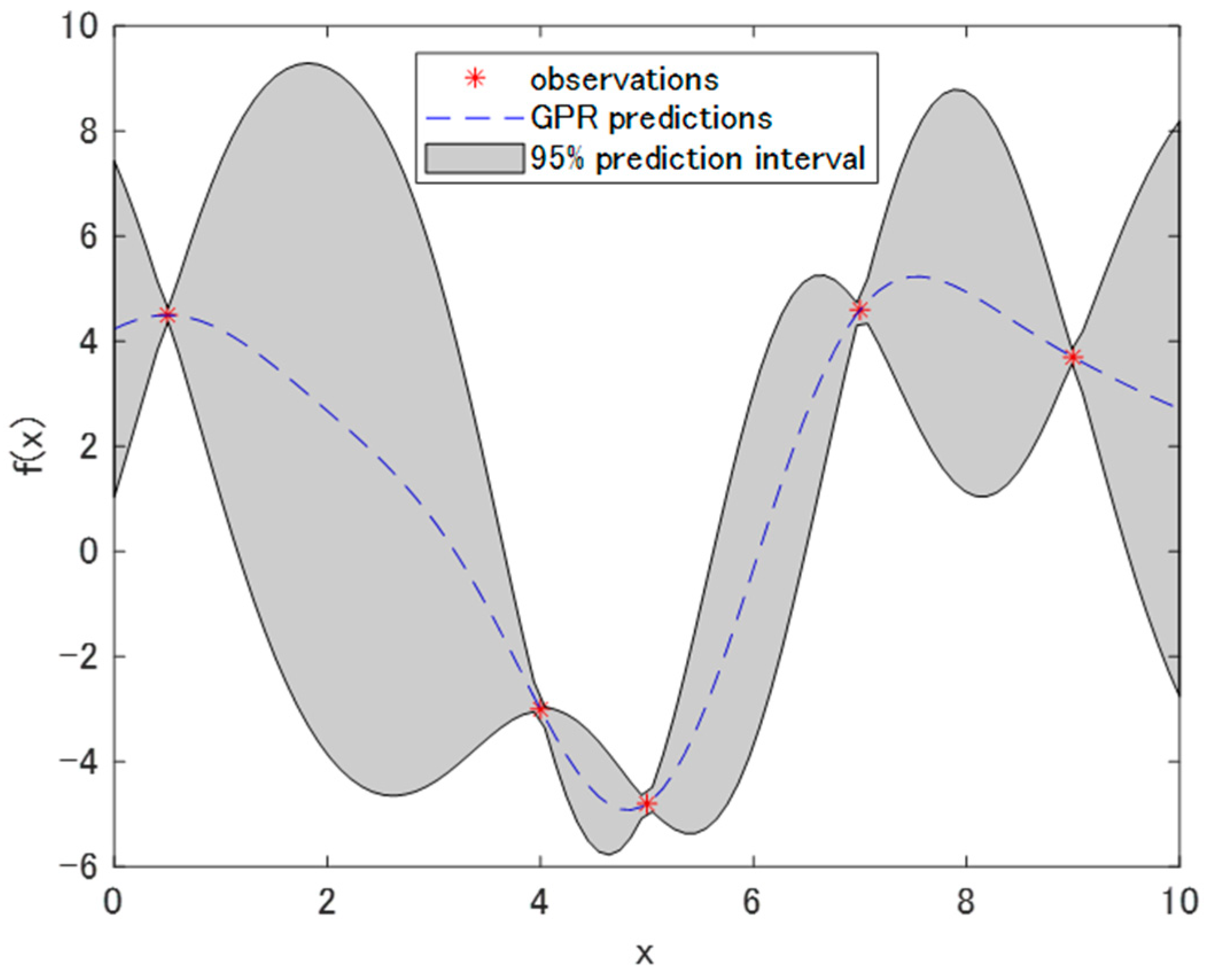
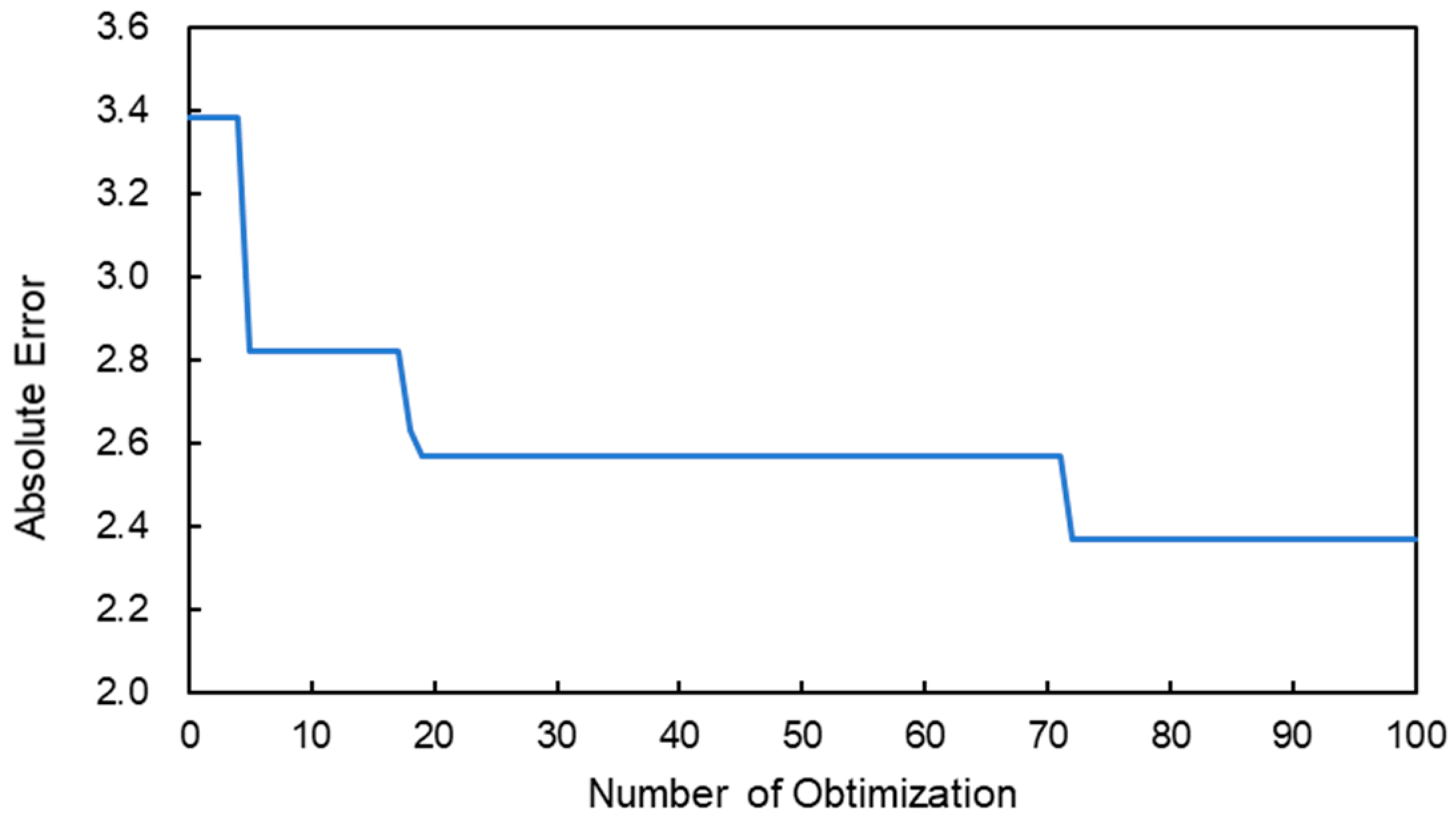
2.3. Bayesian Optimization

In CNN regression, what we have to optimize is a black box function, which means, when querying at a point x, its expected value and divergence cannot be estimated. Thus, in Bayesian optimization, we assume that the function to be optimized follows a stochastic process. The Gaussian process is commonly used as a stochastic process. For instance, consider that five observations derived from a black box function f(x) are available. Then, the performance of the Gaussian process regression is indicated in Figure 3 [26,27]. In Figure 3, the dotted line illustrates the result of the predictions via a Gaussian process regression. This line represents the estimated value of the function that has the largest possibility. The patched area with grey depicts that with a percentage of 95%, and the value of the function is within the area. Each extracted graph in a vertical direction at a certain x value describes the Gaussian distribution.

In Bayesian optimization, the best point that contains the higher (or lower) value is estimated; then, a Gaussian process regression is performed including the new observation. By continuing this procedure (in this study, 100 times), optimized parameters are found. The next point to be selected is determined based on the acquisition function that considers both the expected value and variance. When searching around an area where estimation value is highest, it is likely that other high values can be obtained. However, only searching around the area leads to the local maximum, not the global maximum. Therefore, the next point should be selected considering the variance of the estimated value. We define the functions $m\left(x\right)$ and $\sigma \left(x\right)$, which are related to the mean and variance of the objective, respectively; then, using an acquisition function $m\left(x\right)+ \sigma \left(x\right)$ the next point is decided [28]. In this study, the expected improvement was adopted for the acquisition function [29].

Here, the parameters considered to be influential for the result, namely initial learn rate, momentum, factor of L₂ regulation (weight decay) [30], the number of filters for convolution, and network depth, were optimized.

2.4. Evaluation of the Brix/Acid Ratio Estimation with Deep Learning

For evaluating the estimation accuracy of Brix/acid ratio with CNN regression, the absolute error of the estimation was calculated. Then, to ensure its high accuracy, the estimation error with the two methods proposed by Muharfiza et al. [11] was calculated with cross-validation. Moreover, principal component regression (PCR), which has been utilized for the analysis of EEM spectra [31] was conducted for the estimation.

Next, to investigate the impact of each region used in EEM on the estimation with CNN, the EEM data was divided into four parts, namely whose range of emission wavelength was 300–400 nm, 400–500 nm, 500–600 nm, and 600–700 nm. With each split EEM data, the CNN regression explained above was conducted and the estimation accuracy with each split data was calculated.

3. Results and Discussion

Figure 4 shows the relationship between the number of parameter optimizations and the minimum absolute error of the Brix/acid ratio. As the number of the optimizations increased, the minimum absolute error of the estimation decreased. A similar result was obtained when the same optimization was conducted again.

Table 1. Optimized architecture for CNN regression for the Brix/acid ratio estimation.

Name	Explanation
Image Input Layer	Image size: 32 × 32
Convolution Layer 1	Number of filter: 37, Filter size: 3 × 3, Stride: [1 1]
Batch Normalization 1	Batch normalization with 37 channels
Relu Layer 1	−
Maxpooling Layer 1	2 × 2 max pooling with stride [2 2], Padding: [0 0]
Convolution Layer 2	Number of filter: 74, Filter size: 3 × 3 Stride: [1 1]
Batch Normalization 2	Batch normalization with 74 channels
Relu Layer 2	−
Maxpooling Layer 2	2 × 2 max pooling with stride [2 2], Padding: [0 0]
Convolution Layer 3	Number of filter: 148, Filter size: 3 × 3, Stride: [1 1]
Batch Normalization 3	Batch normalization with 148 channels
Relu Layer 3	-
Average Pooling 1	8 × 8 Average pooling with stride [2 2], Padding: [0 0]
Dropout	20% Dropout
Fully Connected Layer	One fully connected layer
Regression Layer	Regression (to minimize mean-squared error)

shows the optimized architecture of the CNN regression for the Brix/acid ratio estimation. The optimized network had three layers. Generally, as the depth of the network increased, the convolutional neural network could express more, resulting in a higher accuracy. For example, to cover various types of images (1000-class) for classification, deeper networks, such as Alexnet and GoogLeNet, have been developed [32,33]. However, if the depth is deeper, the network is easier to over-tune for the training data and the estimation accuracy decreases. Moreover, deeper networks necessitate a longer calculation time. However, for the specific task, that is, the Brix/acid ratio estimation of citrus, efficient learning can be done without using such a deep network. The advantage of the use of a non-deep network is that the time and cost for the deep learning can be reduced. Further, if the network architecture is optimized, fewer training data are necessary, which results in a reduction in the cost of collecting training data. In deep learning, one of the biggest challenges is gathering sufficient and high quality data. The network optimization for the CNN regression will help in obtaining an efficient and accurate quantitative estimation. To date, studies that consider hyperparameters well and optimize the network are limited, especially in evaluating agricultural products or plants. Like this study, it is desirable to optimize those parameters using Bayesian optimization in the fields.

Table 2. Brix/Acid ratio estimation result with previous methods and the present method. Methods (1) and (2) are proposed by Muharfiza et al. (2017).

	Estimation Method	Absolute Estimation Error of Brix/Acid Ratio
1	Two peaks of polymethoxy flavone	6.21
2	Two peaks of Tryptophan and Chlorophyll	4.49
3	PCR (Principal Component Regression)	4.04
4	Present method (CNN regression)	2.48

shows the absolute error of the Brix/acid ratio with previous estimation methods and the present CNN regression. The methods (1) and (2) in the table were proposed by Muharfiza et al. [11]. The methods (3) and (4) were PCR and the current CNN regression. Their absolute errors were 6.21, 4.49, 4.04, and 2.48, respectively. The present CNN regression (method (4)) had a much higher estimation accuracy. The previous methods, (1) and (2), used only two types of peak height. In method (3), PCR, the useful information for Brix/acid ratio estimation was extracted. In the CNN regression, the information of small peaks, the evenness of the spectrum, and shoulder intensity were considered added to the fluorescence peak intensity. Further, the network was composed of many filters and layers that transformed the input data to output, while leaning on increasingly higher-level features [34]; these factors resulted in higher accuracy. The amount of data for the CNN regression was 141 in total, and it is comparatively less in deep learning. For example, in image classification, each target image did not have the same position; hence, even if the images belonged to the same category, the location of each important part (e.g., flower, leaf, and leaf vein) would be different, which demanded considerably more training images to cover the position and other differences, such as brightness. In contrast, in this study, EEM was inputted as a training image in which the fluorescence peaks were recorded at the same position every time. It does not require the consideration of the difference of the position and other factors, resulting in a high accuracy with a comparatively less amount of data.

Table 3. Absolute error of the Brix/Acid ratio with CNN regression when the EEM area for estimation is limited and the other areas are masked. The range of emission wavelength used for the estimation was (A) 300–400 nm, (B) 400–500 nm, (C) 500–600 nm, and (D) 600–700 nm.

Range of Excitation Wavelength Used for the Estimation	Absolute Estimation Error of Brix/Acid Ratio
(A) 300–400 nm	3.66
(B) 400–500 nm	5.85
(C) 500–600 nm	4.23
(D) 600–700 nm	3.1
300–700 nm (full range)	2.48

shows the absolute error of the Brix/acid ratio with CNN regression when the EEM area for the estimation was limited and other areas were masked. When the range of emission wavelength was used as (A) 300–400 nm, (B) 400–500 nm, (C) 500–600 nm, and (D) 600–700 nm, the estimation error was observed to be 3.66, 5.85, 4.23, and 3.10, respectively; when using the full range, the estimation error was 2.48. The estimation error was greatest in area B, which did not have any peaks. The fluorescent peaks observed in the range (B) and (D) were from polymethoxy flavone [35,36] and chlorophyll, respectively. With a different cultivar of citrus, the fluorescence substance in area (A) was derived from tryptophan [37]. Using thin-layer chromatography and nuclear magnetic resonance, we confirmed that tryptophan was also present in the citrus unshu, which was used in this study. From these reasons, it was implied that the fluorescence peak of tryptophan and chlorophyll contributed to the high accuracy. According to Muharfiza et al. [11], the peak of tryptophan was useful for the Brix/acid ratio estimation. The result in this study with CNN regression agreed with the previous study [11]. Moreover, in terms of plant physiology, it is suggested that the amount of amino acid would be a good indicator of citrus maturity [38]. Learning through CNN would capture the features that are biologically important and realize high accuracy.

As Table 2 represents, not using a specific peak but using all peaks, high accuracy was achieved. With more samples, this result will be more reliable, and it is likely that the estimation accuracy will increase.

4. Conclusions

In this study, fluorescence measurement of extracted citrus peel was conducted and a regression with CNN (CNN regression) was performed to estimate the Brix/acid ratio of juice from the flesh accurately. The EEM obtained from the fluorescence measurement was regarded as an image, which allowed for the CNN regression. As a result, the Brix/acid ratio absolute error was estimated to be 2.48, which is considerably better than the values obtained by the other methods in previous studies. Not only was this an appropriate method for the prediction, but we also conducted Bayesian optimization to choose hyper-parameters in the deep neural network. Due to the optimization, the determination of the parameters could be done automatically and appropriately. Furthermore, it was found that the optimization itself contributed to the high accuracy. Added to the maturity estimation of other fruits, the method to perform a CNN regression would be available for detecting the extent of mechanical damage and infections of agricultural products. This CNN regression method offers precise quantitative estimation of fruit quality, and it can be applied to a wide variety of fields.

References

1. Ministry of Agriculture, Forestry and Fisheries. The Situation Surrounding Fruits. Available online: http://www.maff.go.jp/j/seisan/ryutu/fruits/attach/pdf/index-57.pdf (accessed on 20 November 2018).
2. Morimoto, T.; Chikaizumi, S.; Hashimoto, Y. Intelligent quality control of fruit storage factory. J. Shita 1994, 6, 191–196. [Google Scholar]
3. Momin, A.M.; Kondo, N.; Ogawa, Y.; Shiigi, T.; Kurita, M.; Ninomiya, K. Machine vision system for detecting fluorescent area of citrus using fluorescence image. Proc. IFAC 2010, 43, 241–244. [Google Scholar] [CrossRef]
4. Reid, M.S. Maturation and maturity indices. In Postharvest Technology of Horticultural Crops; University of California Division of Agriculture and Natural Resources Publication: Oakland, CA, USA, 2002; pp. 21–28. [Google Scholar]
5. Cary, P.R. Citrus Fruit Maturity; MPKV: Rahuri, India, 1974; p. 26. [Google Scholar]
6. Iglesias, D.J.; Cercós, M.; Colmenero-Flores, J.M.; Naranjo, M.A.; Ríos, G.; Carrera, E.; Ruiz-Rivero, O.; Lliso, I.; Morillon, R.; Tadeo, F.R.; et al. Physiology of citrus fruiting. Braz. J. Plant Physiol. 2007, 19, 333–362. [Google Scholar] [CrossRef]
7. Kimball, D. Citrus Processing: Quality Control and Technology; Springer Science & Business Media: New York, NY, USA, 1991; p. 55. [Google Scholar]
8. Kondo, N.; Ahmad, U.; Monta, M.; Murase, H. Machine vision based quality evaluation of Iyokan orange fruit using neural networks. Comput. Electron. Agric. 2000, 29, 135–147. [Google Scholar] [CrossRef]
9. Antonucci, F.; Pallottino, F.; Paglia, G.; Palma, A.; D’Aquino, S.; Menesatti, P. Non-destructive estimation of mandarin maturity status through portable VIS-NIR spectrophotometer. Food Bioprocess. Technol. 2011, 4, 809–813. [Google Scholar] [CrossRef]
10. Christensen, J.; Povlsen, V.T.; Sørensen, J. Application of fluorescence spectroscopy and chemometrics in the evaluation of processed cheese during storage. J. Dairy Sci. 2003, 86, 1101–1107. [Google Scholar] [CrossRef]
11. Muharfiza; Riza, A.F.D.; Saito, Y.; Itakura, K.; Kohno, Y.; Suzuki, T.; Kuramoto, M.; Kondo, N. Monitoring of Fluorescence Characteristics of Satsuma Mandarin (Citrus unshiu Marc.) during the Maturation Period. Horticulturae 2017, 3, 51. [Google Scholar] [CrossRef]
12. Wang, X.; Cao, L.; Yang, S.T.; Lu, F.; Meziani, M.J.; Tian, L.; Sun, K.W.; Bloodgood, M.A.; Sun, Y.P. Bandgap-Like strong fluorescence in functionalized carbon nanoparticles. Angew. Chem. Int. Ed. 2010, 49, 5310–5314. [Google Scholar] [CrossRef]
13. Sugiyama, J.; Tsuta, M. Discrimination and quantification thechnology for food using fluorescence fingerprint. Nippon Shokuhin Kagaku Kogaku Kaishi 2013, 60, 457–465. [Google Scholar] [CrossRef]
14. Maggiori, E.; Tarabalka, Y.; Charpiat, G.; Alliez, P. Convolutional neural networks for large-scale remote-sensing image classification. IEEE Trans. Geosci. Remote Sens. 2017, 55, 645–657. [Google Scholar] [CrossRef]
15. Barbedo, J.G.A. Impact of dataset size and variety on the effectiveness of deep learning and transfer learning for plant disease classification. Comput. Electron. Agric. 2018, 153, 46–53. [Google Scholar] [CrossRef]
16. Barbedo, J.G.A. Factors influencing the use of deep learning for plant disease recognition. Biosyst. Eng. 2018, 172, 84–91. [Google Scholar] [CrossRef]
17. Itakura, K.; Hosoi, F. Estimation of tree structural parameters from video frames with removal of blurred images using machine learning. J. Agric. Meteorol. 2018, 74, 154–161. [Google Scholar] [CrossRef]
18. Suh, H.K.; Ijsselmuiden, J.; Hofstee, J.W.; van Henten, E.J. Transfer learning for the classification of sugar beet and volunteer potato under field conditions. Biosyst. Eng. 2018, 174, 50–65. [Google Scholar] [CrossRef]
19. Miao, S.; Wang, Z.J.; Liao, R. A CNN regression approach for real-time 2D/3D registration. IEEE Trans. Med. Imaging 2016, 35, 1352–1363. [Google Scholar] [CrossRef]
20. Deng, L.; Hinton, G.; Kingsbury, B. New types of deep neural network learning for speech recognition and related applications: An overview. In Proceedings of the 2013 IEEE International Conference on Acoustics, Speech and Signal Processing (ICASSP), Vancouver, BC, Canada, 26–31 May 2013; pp. 8599–8603. [Google Scholar]
21. Aloysius, N.; Geetha, M. A review on deep convolutional neural networks. In Proceedings of the 2017 International Conference on Communication and Signal Processing (ICCSP 2017), Chennai, India, 6–8 April 2017; pp. 0588–0592. [Google Scholar]
22. Močkus, J. On Bayesian methods for seeking the extremum. In Proceedings of the Optimization Techniques IFIP Technical Conference, Novosibirsk, Russia, 1–7 July 1975; Springer: Berlin, Heidelberg, 1975; pp. 400–404. [Google Scholar]
23. Zhang, Y.; Sohn, K.; Villegas, R.; Pan, G.; Lee, H. Improving object detection with deep convolutional networks via bayesian optimization and structured prediction. In Proceedings of the IEEE Conference on Computer Vision and Pattern Recognition, Boston, MA, USA, 7–12 June 2015; pp. 249–258. [Google Scholar]
24. Rawat, W.; Wang, Z. Deep convolutional neural networks for image classification: A comprehensive review. Neural Comput. 2017, 29, 2352–2449. [Google Scholar] [CrossRef]
25. Gong, Y.; Jia, Y.; Leung, T.; Toshev, A.; Ioffe, S. Deep convolutional ranking for multilabel image annotation. arXiv, 2013; arXiv:1312.4894. [Google Scholar]
26. Locatelli, M. Bayesian algorithms for one-dimensional global optimization. J. Glob. Optim. 1997, 10, 57–76. [Google Scholar] [CrossRef]
27. Brochu, E.; Cora, M.; de Freitas, N.A. Tutorial on Bayesian Optimization of Expensive Cost Functions, with Application to Active User Modeling and Hierarchical Reinforcement Learning; Technical Report TR-2009-23; Department of Computer Science, University of British Columbia: Vancouver, BC, Canada, 2009. [Google Scholar]
28. Kano, M.; Yoshizaki, R. Operating condition optimization for efficient scale-up of manufacturing process by using Bayesian optimization and transfer learning. J. SICI 2017, 56, 695–698. [Google Scholar]
29. Snoek, J.; Larochelle, H.; Adams, R.P. Practical Bayesian Optimization of Machine Learning Algorithms. 2012, 2, pp. 2951–2959. Available online: http://papers.nips.cc/paper/4522-practical-bayesian-optimization (accessed on 20 November 2018).
30. Goodfellow, I.; Bengio, Y.; Courville, A. Deep Learning; MIT Press: Cambridge, UK, 2016. [Google Scholar]
31. Syukri, D.; Thammawong, M.; Naznin, H.A.; Kuroki, S.; Tsuta, M.; Yoshida, M.; Nakano, K. Identification of a freshness marker metabolite in stored soybean sprouts by comprehensive mass-spectrometric analysis of carbonyl compounds. Food Chem. 2018, 269, 588–594. [Google Scholar] [CrossRef]
32. Krizhevsky, A.; Sutskever, I.; Hinton, G.E. Imagenet classification with deep convolutional neural networks. NIPS 2012, 60, 84–90. [Google Scholar] [CrossRef]
33. Szegedy, C.; Liu, W.; Jia, Y.; Sermanet, P.; Reed, S.; Anguelov, D.; Erhan, D.; Vanhoucke, V.; Rabinovich, A. Going deeper with convolutions. In Proceedings of the 28th IEEE Conference on Computer Vision and Pattern Recognition, Boston, MA, USA, 7–12 June 2015; pp. 1–9. [Google Scholar]
34. Litjens, G.; Kooi, T.; Bejnordi, B.E.; Setio, A.A.A.; Ciompi, F.; Ghafoorian, M.; van der Laak, J.A.W.M.; Van Ginneken, B.; Sánchez, C.I. A survey on deep learning in medical image analysis. Med. Image Anal. 2017, 42, 60–88. [Google Scholar] [CrossRef] [Green Version]
35. Slaughter, D.C.; Obenland, D.M.; Thompson, J.F.; Arpaia, M.L.; Margosan, D.A. Non-destructive freeze damage detection in oranges using machine vision and ultraviolet fluorescence. Postharvest Biol. Technol. 2008, 48, 341–346. [Google Scholar] [CrossRef]
36. Ogawa, Y.; Momin, A.M.; Kuramoto, M.; Kohno, Y.; Shiigi, T.; Yamamoto, K.; Kondo, N. Detection of rotten citrus fruit using fluorescent images. Rev. Laser Eng. 2011, 39, 255–261. [Google Scholar] [CrossRef]
37. Sun, Y.; Zhang, H.; Sun, Y.; Zhang, Y.; Liu, H.; Cheng, J.; Bi, S.; Zhang, H. Study of interaction between protein and main active components in Citrus aurantium L. by optical spectroscopy. J. Lumin. 2010, 130, 270–279. [Google Scholar] [CrossRef]
38. Daito, H.; Tominaga, S. Studies on fruit quality of navel oranges and several Japanese late and midseason citrus cultivars in Seto inland sea area IV seasonal changes in amino acid constituents of juice. Bull. Shikoku Agric. Exp. Stn. 1981, 37, 75–85. [Google Scholar]
Figure 1. Example of excitation and emission matrix of extracted citrus peel. The brightness of the color is directly proportional to the fluorescence intensity as the color bar represents. The plus marks show fluorescence peaks.
Horticulturae 05 00002 g001
Figure 2. Flowchart of the experiment. (1) Fluorescence measurement; (2) Actual measurement of Brix/acid ratio.
Horticulturae 05 00002 g002
Figure 3. Example of a Gaussian process regression (dotted line) with five observations. The patched area represents the 95% prediction interval.
Horticulturae 05 00002 g003
Figure 4. Relationship between the number of optimizations and the minimum absolute error of the estimation of the Brix/acid ratio.
Horticulturae 05 00002 g004