A Predictive Model of the Photosynthetic Rate of Chili Peppers Using Support Vector Regression and Environmental Multi-Factor Analysis

Abstract

Light intensity, CO₂ concentration, and temperature are three primary environmental factors with high temporal variability, nonlinearity, and strong coupling, which directly influence the photosynthetic rate of plants. To investigate the combined influence of these factors on the photosynthetic rate of chili pepper plants, a predictive model was developed for their net photosynthetic rate (Pn) during the peak fruiting period. A multifactorial nested experimental design with irregular sampling intervals was used to systematically examine the interacting effects of light intensity, CO₂ concentration, and temperature on photosynthesis. Based on the collected data, a support vector regression (SVR) algorithm was trained and its performance was compared with that of a backpropagation (BP) neural network, a radial basis function (RBF) neural network, and a random forest (RF) algorithm. To optimize performance, a grid search with five-fold cross-validation was conducted to identify optimal hyperparameters; this process yielded a cost parameter (C) of 38 and a gamma parameter (γ) of 8, which minimized the root mean square error (RMSE) on the training set. On the test set, the SVR model achieved a coefficient of determination (R²) of 0.9941 and an RMSE of 0.6988 μmol m⁻² s⁻¹ (relative to the full Pn range of −4.19 to 39.2 μmol m⁻² s⁻¹). A linear fit between measured and predicted Pn values yielded a slope of 0.992 and an intercept of 0.07, indicating near-perfect agreement and surpassing the performance of the BP, RBF, and RF models. These results demonstrate that the SVR-based model outperformed the other approaches and exhibited superior predictive ability, establishing it as a robust theoretical foundation and a practical tool for dynamic environmental optimization in controlled-environment agriculture.

1. Introduction

Facility agriculture is a modern agricultural model based on environmental engineering technology that achieves year-round continuous and efficient production of facility crops by precisely regulating key environmental factors such as light intensity, CO₂ concentration, and temperature within the facility [1]. Compared with traditional open-field agriculture, facility agriculture boasts advantages such as a high degree of automation and production that are not limited by seasons or regions and has gradually developed into a pillar industry of China’s agricultural economy [2]. Internationally, facility agriculture is often referred to as controlled environment agriculture, which is characterized by adjusting the environment in which crops are grown to maintain optimal growth and thus increase yields [3]. Therefore, constructing a photosynthesis model based on multifactor collaborative regulation is crucial for meeting crop photosynthetic demands in facility agriculture. This approach enables analysis of dynamic responses between environmental parameters and net photosynthetic rate (Pn), optimization of growth conditions, and overcoming the ‘bottleneck of environmental regulation’ to achieve efficient, high-quality production [4,5,6].

The photosynthetic rate is an important indicator for assessing photosynthetic efficiency [7], though contemporary research also evaluates quantum yield and chlorophyll fluorescence [8]. Its dynamics are synergistically regulated by three factors: light intensity, CO₂ concentration, and temperature. Light is the energy source for plants to perform photosynthesis, produces oxygen and organic matter, and drives the synthesis of ATP and NADPH in the light reaction [9]. CO₂ serves as the substrate for producing carbohydrates in photosynthesis, acting as an essential raw material [10], and changes in its concentration can also alter the activity of RuBP carboxylase [11]. Temperature directly influences the rates of both light and carbon reactions in photosynthesis by affecting the activity of RuBisCO reactive enzymes and stomatal opening [12]. When the temperature is too low, the activity of the RuBisCO enzyme significantly decreases, leading to a reduction in the rate of carboxylation [13]. In the appropriate temperature range, elevated temperature can significantly increase the activity of RuBisCO and other enzymes related to photosynthesis, as well as increase the fluidity of the cystoid membrane, thus promoting the efficiency of light energy capture and electron transfer in photosystem II [9]. However, when the temperature is excessively high, the thermal inactivation of the RuBisCO leads to a decrease in the maximum carboxylation rate, and the photochemical efficiency of photosystem II also decreases, leading to the dissipation of light energy [14]. To explore the relationships between light intensities, CO₂ concentrations, temperatures, and Pn, it is crucial to establish a multifactor coupled photosynthetic rate prediction model. However, due to the complex interactions among these environmental variables, precise regulation of facility horticulture environments remained a significant challenge [15].

In recent years, significant progress has been made in both theoretical and applied aspects of photosynthetic rate prediction models. Traditional models, such as the FvCB model (a biochemical framework describing photosynthesis based on enzyme kinetics and electron transport), nonrectangular hyperbola model, and modified rectangular hyperbola model, rely primarily on biochemical principles to elucidate the mechanisms of photosynthesis by quantifying parameters such as RuBP carboxylase activity and electron transport efficiency [16]. However, these models require specific biochemical parameters to explain particular photosynthetic responses, making it difficult to comprehensively analyze the nonlinear coupling effects of multiple external environmental factors [17]. Nonetheless, these traditional models have laid an important theoretical foundation for subsequent research on photosynthesis. With the rapid development of machine learning technology, intelligent algorithms have gradually become a new focus for constructing multifactor coupled photosynthetic rate models [18]. Compared with traditional methods, machine learning models significantly improve the prediction accuracy and generalization capabilities by learning from large amounts of environmental parameters and Pn data, using environmental parameters as inputs and predicting Pn as output [19]. Artificial neural networks (ANNs), as algorithms based on biological neural networks, simulate biological brain activities and adaptively adjust weights and thresholds during the learning process, enabling the expression of complex nonlinear relationships [20]. For example, a Pn prediction model for tomato leaves during the flowering period, which is based on a BP neural network, significantly improves the fitting accuracy [21]. However, ANNs have limitations such as slow convergence and long training cycles when dealing with diverse sample problems [22]. In contrast, support vector regression (SVR) maps data to a high dimensional space through kernel functions and seeks the optimal regression hyperplane in this high-dimensional space, offering the advantages of high speed, high accuracy, and strong generalization capabilities [23]. Despite their theoretical value, these models struggled with multifactor coupling analysis. Machine learning algorithms, such as SVR, integrate dynamic interactions across multiple environments and offer new technical pathways for precise environmental regulation in facility horticulture [15].

SVR is a regression algorithm based on support vector machines (SVM), and is primarily used to solve regression problems [24]. As an extension of SVM in the field of regression, SVR seeks an optimal hyperplane to fit the data, minimizing the error between the predicted and actual values within a certain range [25]. The advantages of the SVR algorithm include high versatility, strong generalization capability, robustness [23], and support for nonlinear fitting, allowing it to handle complex nonlinear relationships through kernel functions [26,27]. These characteristics make SVR particularly suitable for modeling the intricate coupling effects of environmental factors on photosynthesis, where traditional biochemical models often struggle with multifactor nonlinear interactions [17]. The regression performance of SVR primarily depends on two aspects: the choice of kernel function, where the radial basis function is widely adopted for its ability to transform low-dimensional nonlinear problems into linearly separable high-dimensional space problems [28]; and the optimization of hyperparameters, where the regularization parameter c balances model complexity against training error, and the kernel parameter g governs data distribution in feature space [29].

The back propagation (BP) neural network is a type of multilayer feedforward neural network trained through the error backpropagation algorithm [30]. It can fit complex nonlinear relationships through multiple layers of nonlinear transformations, offering strong nonlinear modeling capabilities [21]. Additionally, the network’s capacity can be expanded by increasing the number of hidden layers or nodes, making it adaptable to more complex tasks [20]. However, for deep networks or large-scale datasets, the training time may be longer, as each iteration requires forward and backwards propagation, resulting in high computational complexity [21]. The radial basis function (RBF) neural network differs from the globally responsive BP neural network, as it is a locally responsive neural network. When input data are fed into the RBF neural network, only a small number of connection weights are activated to produce a response, which determines the network’s output, resulting in faster training speeds [31]. The network structure also includes an input layer, a hidden layer, and an output layer. Random forest (RF) is a machine learning algorithm based on ensemble learning [32]. It improves model accuracy and robustness by combining the prediction results of multiple decision trees, and it is capable of handling nonlinear relationships and high-dimensional data [33].

Currently, recent advances in photosynthesis modeling have not yet fully addressed the coupled effects of light intensity, CO₂ concentration, and temperature on Pn in facility-cultivated pepper leaves and the construction of predictive models for photosynthetic rates, especially at the fruiting stage. For this reason, this study designed a nested experiment with non-uniform sampling periods for multiple environmental factors using facility-cultivated chili peppers. The Pn dataset of peppers at the peak fruiting period was systematically measured under different combinations of light intensity (measured as photosynthetic light flux density (PPFD)), CO₂ concentration, and temperature. Based on this, a photosynthetic rate prediction model was developed using the SVR algorithm, BP neural network, RBF neural network, and RF algorithm. The study compared and analyzed the differences between these algorithms in terms of convergence speed, prediction accuracy, and generalization ability.

2. Materials and Methods

2.1. Experimental Materials

The experiment was carried out from August to December 2024 in a controlled-environment growth chamber at the Horticultural Experiment Station of Shanxi Agricultural University (112°28′–113°01′ E, 37°12′–37°32′ N; 2023.5 m), which was established by the Modern Agro-Industry Technology Research System of Shanxi Province (Taiyuan, Shanxi, China). Environmental conditions were maintained at a day/night temperature of 28 ± 0.5 °C/18 ± 0.5 °C, a photosynthetic photon flux density of 350–400 μmol m⁻² s⁻¹ under a 12 h photoperiod, and a relative humidity of 55–75%.

The experimental material used was the Huamei 105 pepper variety (Capsicum annuum L., Solanaceae) obtained from Jiuquan Huamei seed industry co. (Jiuquan, Gansu China). Seeds of uniform size and plump morphology were selected and soaked in warm water at 55 °C for 20 min and then left at room temperature for 8 h. The pepper seeds were placed on two layers of sterile gauze (previously soaked in sterile water), wrapped, and placed in a thermostatic incubator at 28 °C for germination. After 7 days, when the seeds germinated, they were sown in 8 × 8 × 5 cm nutrient pots (one seedling per pot). When the plants had 7–8 leaves (about 35 days after germination), 30 healthy seedlings of similar growth status were randomly selected and transplanted into 19 × 17 × 15 cm pots (one seedling per pot). Data collection was conducted during the peak fruiting period (60–75 days after transplanting).

The cultivation and transplantation process were carried out using agricultural-specific substrates with identical nutrient contents. The substrate parameters were as follows: 50% (by mass) organic fertilizer, 20% (by mass) humic acid, and a pH ranging from 5.5 to 6.5. For irrigation, we utilized Hoagland nutrient solution throughout all growth stages. No pesticides or plant growth regulators were used during the entire trial.

2.2. Multienvironmental Factor Nested Experimental Design

The experimental design employed a nested approach with three controlled environmental factors: light intensity, CO₂ concentration, and temperature in the facility environment were used as independent variables, whereas the Pn of pepper leaves served as the dependent variable. To avoid the midday depression of photosynthesis [34], data collection was conducted daily between 09:00 and 11:30 and 14:00 and 17:30. During the nonuniform sampling period, a multigradient nested experiment was designed: PPFD: 14 levels (0, 50, 100, 150, 200, 400, 600, 800, 1000, 1200, 1400, 1600, 1800, 2000 μmol m⁻² s⁻¹); CO₂ concentration: 9 levels (200, 400, 600, 800, 1000, 1200, 1400, 1600, 1800 μmol mol⁻¹); temperature: 10 levels (12, 15, 20, 22, 24, 26, 28, 30, 32, 35 °C). The microenvironmental conditions required for the measurements were created manually using the Li-6400 portable photosynthesis system (Li-COR Biosciences, Lincoln, NE, USA). Among these, the CO₂ concentration injection system was used to increase the CO₂ concentration in the leaf chamber; soda lime tubes were used to reduce the CO₂ concentration; resistance wires were used to increase the leaf chamber temperature; condensers were used to lower the leaf chamber temperature; and a fluorescent light source module was used to control the PPFD value. The red-to-blue light ratio was set to 9:1 by default, the flow rate was set to 500 μmol s⁻¹, and the measurement environment humidity was maintained at 55–75%.

Before measurement, the target leaves were acclimated to light in the leaf chamber for 20–30 min to activate photosynthetic enzymes to obtain stable data. For each combination of temperature (12–35 °C) and CO₂ concentration (200–1800 μmol mol⁻¹), Pn was obtained at 14 PPFD levels (0–2000 μmol m⁻² s⁻¹) by employing a measured light response curve assay. Three fully expanded, unshaded functional leaves from plants with similar growth conditions were selected to measure the Pn under 1260 (14 × 9 × 10) nested combination conditions, resulting in a total of 3780 (1260 × 3) experimental data points. The average of the three repeated measurements was taken as the data result for a given environmental condition, ultimately yielding 1260 experimental datasets.

2.3. Construction of the Photosynthetic Rate Prediction Model

2.3.1. Data Preprocessing

The photosynthesis experimental data reflect the response of environmental conditions to Pn, comprising four dimensions: three features (PPFD, CO₂ concentration, and temperature) and one output (Pn). Therefore, before model training, normalization of sample data across different dimensions is necessary to ensure that data from all dimensions are on the same scale [35]. This prevents sample imbalance due to significant data disparities, which could lead to deviations of the final model from the accurate hyperplane [18]. The normalization process employs a linear normalization method, scaling the data to the interval [0, 1] using Equation (1).

$$Y={\displaystyle \frac{\left(Y_{max}-Y_{min}\right)·\left(X-min\left(X\right)\right)}{max\left(X\right)-min\left(X\right)}}$$

(1)

In this formula [18], min(X) and max(X) represent the minimum and maximum values of the data matrix X, respectively, whereas Y_min and Y_max denote the minimum and maximum values of the target interval. X is the input data matrix and Y represents the normalized data.

After normalization, 70% of the sample data are randomly selected as the training set to train the model, and the remaining 30% are used as the test set to evaluate the model’s performance.

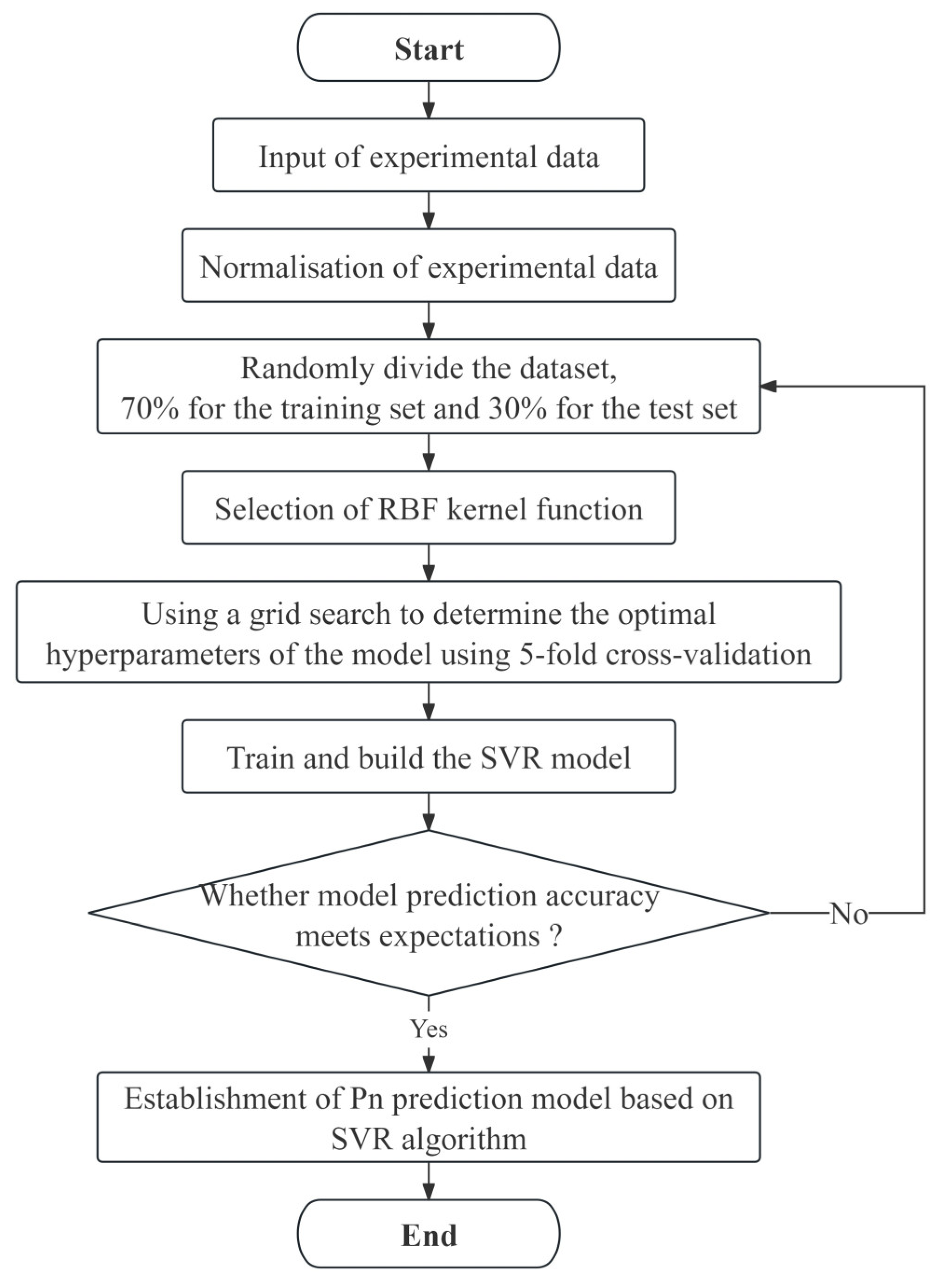
2.3.2. Model Construction

In this study, the RBF kernel function was used for SVR modeling. The hyperparameters (c and γ) were traversed through a grid search over a predetermined range (c: [1–50], g: [1–20], step size 1) and the optimal combination was determined by 5-fold cross-validation to minimize the root mean square error of the training samples. The flowchart for constructing the SVR model in this study is shown in Figure 1, in which the specific steps for modeling the SVR algorithm are as follows:

Step 1: Input Data: $\mathrm{D}=\left({\mathrm{x}}_1,{\mathrm{y}}_1\right),\left({\mathrm{x}}_2,{\mathrm{y}}_2\right),\cdots ,\left({\mathrm{x}}_{\mathrm{n}},{\mathrm{y}}_{\mathrm{n}}\right)$, where each ${\mathrm{x}}_{\mathrm{i}}$ is a three-dimensional feature vector ${\mathrm{x}}_{\mathrm{i}}=\left({\mathrm{x}}_{\mathrm{i}1},{\mathrm{x}}_{\mathrm{i}2},{\mathrm{x}}_{\mathrm{i}3}\right)$ and where ${\mathrm{y}}_{\mathrm{i}}$ is the target value output. Learn a regression function $\mathrm{f}\left(\mathrm{x}\right)$ so that the predicted value $\mathrm{f}\left(\mathrm{x}\right)$ is as close as possible to the true value y.

Step 2: Select the RBF as the kernel function, as in Equation (2).

$$\mathrm{K}\left({\mathrm{x}}_{\mathrm{i}},{\mathrm{x}}_{\mathrm{j}}\right)=\exp \left(-\mathsf{\gamma }\Vert {\mathrm{x}}_{\mathrm{i}}-{\mathrm{x}}_{\mathrm{j}}{\Vert }^2\right)$$

(2)

where γ was the hyperparameter of the kernel function, controlling the width of the Gaussian function.

Step 3: Define the form of the regression function, as in Equation (3).

$$\mathrm{f}\left(\mathrm{x}\right)={\displaystyle \sum }_{\mathrm{i}=1}^{\mathrm{n}}\left({\mathsf{\alpha }}_{\mathrm{i}}-{\mathsf{\alpha }}_{\mathrm{i}}^{*}\right)\mathrm{K}\left({\mathrm{x}}_{\mathrm{i}},\mathrm{x}\right)+\mathrm{b}$$

(3)

${\mathsf{\alpha }}_{\mathrm{i}}$ and ${\mathsf{\alpha }}_{\mathrm{i}}^{*}$ were Lagrange multipliers and b was the bias term.

Step 4: Define the ϵ-insensitive band: If the deviation between the predicted value $\mathrm{f}\left(\mathrm{x}\right)$ and the true value y is within the ϵ range (i.e., $\left|\mathrm{y}-\mathrm{f}\left(\mathrm{x}\right)\right|\le ϵ$), the prediction is considered accurate, and no loss is calculated. If the deviation exceeds ϵ, the loss is computed.

Step 5: Introduce slack variables ${\mathsf{\xi }}_{\mathrm{i}}$ and ${\mathsf{\xi }}_{\mathrm{i}}^{*}$. ${\mathsf{\xi }}_{\mathrm{i}}$ represents the portion where the true value ${\mathrm{y}}_{\mathrm{i}}$ is higher than the predicted value $\mathrm{f}\left({\mathrm{x}}_{\mathrm{i}}\right)+ϵ$, and ${\mathsf{\xi }}_{\mathrm{i}}^{*}$ represents the portion where the true value ${\mathrm{y}}_{\mathrm{i}}$ is lower than the predicted value $\mathrm{f}\left({\mathrm{x}}_{\mathrm{i}}\right)-ϵ$.

Step 6: Construct the optimization objective for SVR: Minimize, as in Equation (4).

$${\displaystyle \frac{1}{2}}\Vert \mathrm{w}{\Vert }^2+\mathrm{C}{\displaystyle \sum }_{\mathrm{i}=1}^{\mathrm{n}}\left({\mathsf{\xi }}_{\mathrm{i}}+{\mathsf{\xi }}_{\mathrm{i}}^{*}\right)$$

(4)

The first term ${\displaystyle \frac{1}{2}}\Vert \mathrm{w}{\Vert }^2$ controlled the complexity of the model and the second term $\mathrm{C}{\displaystyle \sum }_{\mathrm{i}=1}^{\mathrm{n}}\left({\mathsf{\xi }}_{\mathrm{i}}+{\mathsf{\xi }}_{\mathrm{i}}^{*}\right)$ was the loss term, which measured the error beyond the ϵ-band. C was the regularization parameter, balancing model complexity and training error.

Step 7: Use the Lagrange multiplier method to transform the optimization problem into a dual problem:

Maximize, as in Equation (5).

$$\mathrm{L}\left(\mathsf{\alpha },{\mathsf{\alpha }}^{*}\right)=-{\displaystyle \frac{1}{2}}{\displaystyle \sum }_{\mathrm{i}=1}^{\mathrm{n}}{\displaystyle \sum }_{\mathrm{j}=1}^{\mathrm{n}}\left({\mathsf{\alpha }}_{\mathrm{i}}-{\mathsf{\alpha }}_{\mathrm{i}}^{*}\right)\left({\mathsf{\alpha }}_{\mathrm{j}}-{\mathsf{\alpha }}_{\mathrm{j}}^{*}\right)\mathrm{K}\left({\mathrm{x}}_{\mathrm{i}},{\mathrm{x}}_{\mathrm{j}}\right)-ϵ{\displaystyle \sum }_{\mathrm{i}=1}^{\mathrm{n}}\left({\mathsf{\alpha }}_{\mathrm{i}}+{\mathsf{\alpha }}_{\mathrm{i}}^{*}\right)+{\displaystyle \sum }_{\mathrm{i}=1}^{\mathrm{n}}{\mathrm{y}}_{\mathrm{i}}\left({\mathsf{\alpha }}_{\mathrm{i}}-{\mathsf{\alpha }}_{\mathrm{i}}^{*}\right)$$

(5)

Subject Equation (6).

$${\displaystyle \sum }_{\mathrm{i}=1}^{\mathrm{n}}\left({\mathsf{\alpha }}_{\mathrm{i}}-{\mathsf{\alpha }}_{\mathrm{i}}^{*}\right)=0, 0\le {\mathsf{\alpha }}_{\mathrm{i}},{\mathsf{\alpha }}_{\mathrm{i}}^{*}\le \mathrm{C}$$

(6)

A quadratic programming (QP) solver was used to solve the above dual problem, and the Lagrange multipliers ${\mathsf{\alpha }}_{\mathrm{i}}$ and ${\mathsf{\alpha }}_{\mathrm{i}}^{*}$ are obtained.

Step 8: Determine the support vectors: Support vectors are data points that satisfy ${\mathsf{\alpha }}_{\mathrm{i}}>0$ or ${\mathsf{\alpha }}_{\mathrm{i}}^{*}>0$. These data points lie on the boundary or outside the ϵ-insensitive band and contribute significantly to the model.

Step 9: Calculate the bias term b, as in Equations (7) and (8).

$$\mathrm{b}={\mathrm{y}}_{\mathrm{j}}-{\displaystyle \sum }_{\mathrm{i}=1}^{\mathrm{n}}\left({\mathsf{\alpha }}_{\mathrm{i}}-{\mathsf{\alpha }}_{\mathrm{i}}^{*}\right)\mathrm{K}\left({\mathrm{x}}_{\mathrm{i}},{\mathrm{x}}_{\mathrm{j}}\right)+ϵ (\mathrm{For} {\mathsf{\alpha }}_{\mathrm{j}}>0)$$

(7)

$$\mathrm{b}={\mathrm{y}}_{\mathrm{j}}-{\displaystyle \sum }_{\mathrm{i}=1}^{\mathrm{n}}\left({\mathsf{\alpha }}_{\mathrm{i}}-{\mathsf{\alpha }}_{\mathrm{i}}^{*}\right)\mathrm{K}\left({\mathrm{x}}_{\mathrm{i}},{\mathrm{x}}_{\mathrm{j}}\right)-ϵ (\mathrm{For} {\mathsf{\alpha }}_{\mathrm{i}}^{*}>0)$$

(8)

Step 10: Construct the final regression function, as in Equation (9).

$$\mathrm{f}\left(\mathrm{x}\right)={\displaystyle \sum }_{\mathrm{i}=1}^{\mathrm{n}}\left({\mathsf{\alpha }}_{\mathrm{i}}-{\mathsf{\alpha }}_{\mathrm{i}}^{*}\right)\mathrm{K}\left({\mathrm{x}}_{\mathrm{i}},\mathrm{x}\right)+\mathrm{b}$$

(9)

where $\mathrm{K}\left({\mathrm{x}}_{\mathrm{i}},\mathrm{x}\right)$ was the RBF kernel function.

Step 11: For a new input vector ${\mathrm{x}}_{\mathrm{i}}=\left({\mathrm{x}}_1,{\mathrm{x}}_2,{\mathrm{x}}_3\right)$, use the regression function $\mathrm{f}\left(\mathrm{x}\right)$ to calculate the predicted value, as in Equation (10).

$${\mathrm{y}}_{\mathrm{pred}}=\mathrm{f}\left(\mathrm{x}\right)$$

(10)

To verify the reliability and accuracy of the SVR model, this study also employed the BP neural network, RBF neural network, and RF algorithm to construct photosynthetic rate prediction models. The same training and test sets used for the SVR algorithm were utilized for modeling and prediction.

For the BP neural network, the model architecture consisted of three input layer neurons (corresponding to PPFD, CO₂ concentration, and temperature) and one output layer neuron (Pn). The Tansig and Purelin functions were selected as activation functions, while the Trainlm function served as the training function [29]. To optimize the model performance, Bayesian optimization was employed to determine the best combination of hyperparameters, including the number of hidden layer nodes (search range: 5–50), learning rate (0.01–0.1), and number of iterations (100–1000). The performance of each hyperparameter set was evaluated using 5-fold cross-validation, and the optimal configuration was selected for the final model training.

Following the same optimization framework used for the BP neural network, the RBF neural network was designed with three input neurons and one output neuron. The hidden layer utilized the RBF as the activation function, transforming low-dimensional input data into a high-dimensional space to enable nonlinear curve fitting [36]. The Bayesian optimization method was also applied to fine-tune the RBF spread parameter, with a search range of 10–100. Model performance was assessed via 5-fold cross-validation, and the optimal spread parameter was identified to train the final RBF model.

For the RF algorithm, a grid search combined with 5-fold cross-validation was conducted to determine the optimal hyperparameters. The search space included the number of decision trees (50–100, step size 10) and the minimum leaf size (5–20, step size 5). The best-performing hyperparameter combination was selected to train the RF model, ensuring robust prediction accuracy.

2.3.3. Model Evaluation Metrics

The coefficient of determination (R²), root mean square error (RMSE), maximum absolute error (MAE), mean bias error (MBE), and mean absolute percentage error (MAPE) are used to evaluate the performance of each prediction model, thereby identifying the optimal photosynthetic rate prediction model. The formulas are as follows (11)–(15).

$${\mathrm{R}}^2=1-{\displaystyle \frac{{{\displaystyle \sum }}_{\mathrm{i}=1}^{\mathrm{n}}{\left({\mathrm{y}}_{\mathrm{i}}-{\hat{\mathrm{y}}}_{\mathrm{i}}\right)}^2}{{{\displaystyle \sum }}_{\mathrm{i}=1}^{\mathrm{n}}{\left({\mathrm{y}}_{\mathrm{i}}-\overline{\mathrm{y}}\right)}^2}}$$

(11)

$$\mathrm{RMSE}=\sqrt{{\displaystyle \frac{1}{\mathrm{n}}}{\displaystyle \sum }_{\mathrm{i}=1}^{\mathrm{n}}{\left({\mathrm{y}}_{\mathrm{i}}-{\hat{\mathrm{y}}}_{\mathrm{i}}\right)}^2}$$

(12)

$$\mathrm{MAE}=\max \left(\left|{\mathrm{y}}_{\mathrm{i}}-{\hat{\mathrm{y}}}_{\mathrm{i}}\right|\right)$$

(13)

$$\mathrm{MBE}={\displaystyle \frac{1}{\mathrm{n}}}{\displaystyle \sum }_{\mathrm{i}=1}^{\mathrm{n}}\left({\mathrm{y}}_{\mathrm{i}}-{\hat{\mathrm{y}}}_{\mathrm{i}}\right)$$

(14)

$$\mathrm{MAPE}={\displaystyle \frac{1}{\mathrm{n}}}{\displaystyle \sum }_{\mathrm{i}=1}^{\mathrm{n}}\left|{\displaystyle \frac{{\mathrm{y}}_{\mathrm{i}}-{\hat{\mathrm{y}}}_{\mathrm{i}}}{{\mathrm{y}}_{\mathrm{i}}}}\right|\times 100\%$$

(15)

where ${\mathrm{y}}_{\mathrm{i}}$, ${\hat{\mathrm{y}}}_{\mathrm{i}}$, and n represent the true values of the model, the predicted values, and the sample size, respectively.

2.4. Software Implementation and Data Visualization

All modeling algorithms in this study, including SVR, the BP neural network, RBF neural network, and RF, were implemented using MATLAB R2024a (MathWorks, Natick, MA, USA). Bayesian optimization and lattice search procedures were implemented using MATLAB’s built-in optimization and machine learning toolbox. Normalization of the input data and computation of the evaluation metrics (R², RMSE, MAE, MBE, and MAPE) were also implemented using custom MATLAB scripts.

The three-dimensional scatter plots illustrating the effects of environmental conditions (PPFD, CO₂ concentration, and temperature) on Pn were generated using Origin 2024 (OriginLab Corporation, Northampton, MA, USA).

3. Results

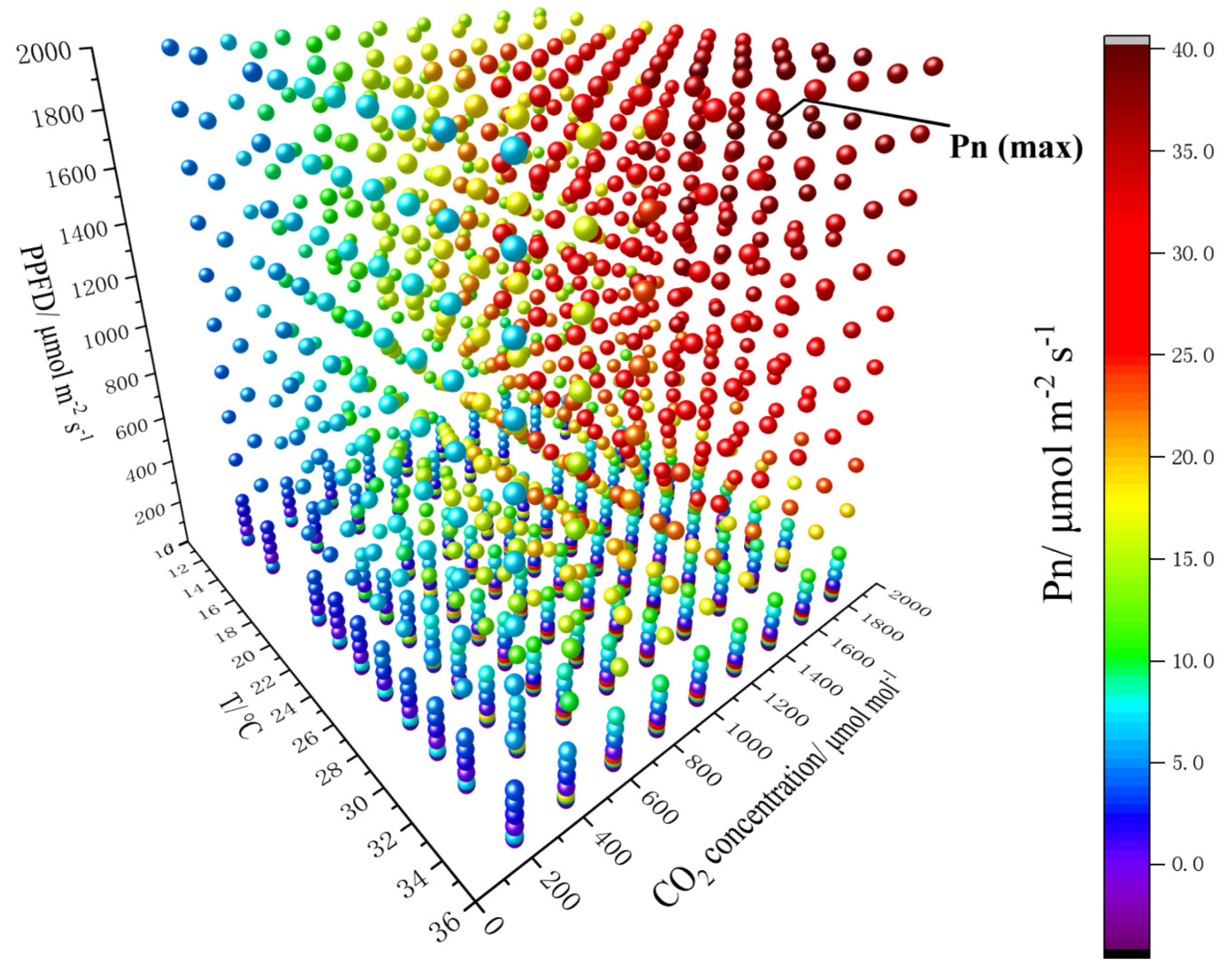
3.1. Impact of Environmental Factors on the Net Photosynthetic Rate

According to the experimental dataset, the maximum Pn (39.2 μmol m⁻² s⁻¹) was achieved under the following optimal environmental conditions: PPFD of 1800 μmol m⁻² s⁻¹, CO₂ concentration of 1600 μmol mol⁻¹, and temperature of 30 °C (Figure 2). To elucidate the relationships between various environmental factors and the Pn, a three-dimensional scatter plot was generated based on the experimental dataset. Under lower temperature conditions (below 20 °C), the Pn was relatively low and rapidly reached saturation. As the temperature increased, the Pn gradually increased. However, when the temperature exceeded 30 °C, the Pn began to decrease. Similarly, under the conditions of constant temperature and CO₂ concentration, the response of Pn to PPFD showed a nonlinear characteristic, initially increasing rapidly with the increase in PPFD and then gradually stabilizeding. Under the conditions of increasing CO₂ concentration and constant temperature and PPFD, Pn also showed the same response trend, with an initial rapid increase, followed by a gradual slowing down of the rate of increase, and finally stabilization.

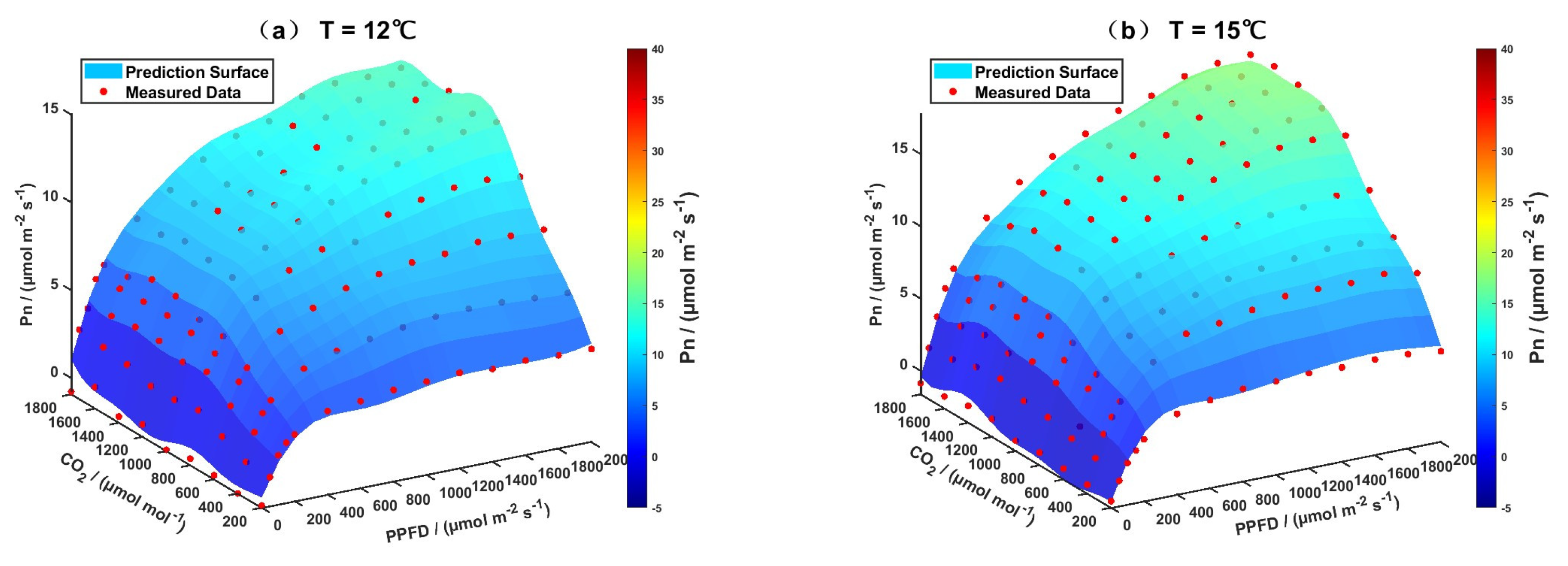
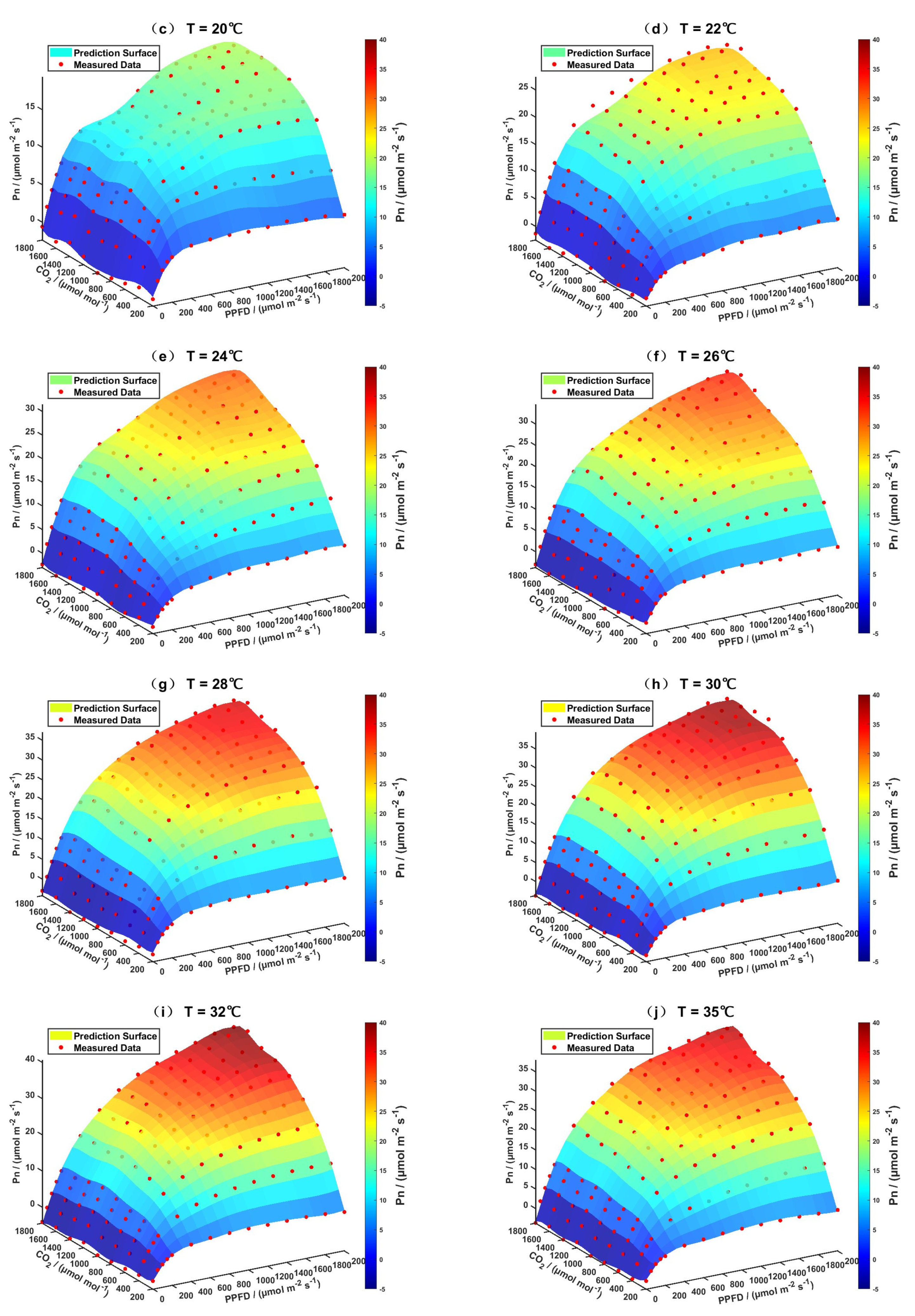
3.2. Model Prediction Results

3.2.1. Evaluation of the Support Vector Regression Model

The optimal hyperparameter combination for the SVR model (c = 38, γ = 8) was determined by grid search and 5-fold cross-validation. Model predictions showed high agreement with measured values across the experimental range (temperature: 12–35 °C, CO₂ concentration: 200–1800 μmol mol⁻¹, PPFD: 0–2000 μmol m⁻² s⁻¹), demonstrating excellent predictive ability (Figure 3). This visual comparison between predicted surfaces and experimental measurements confirms the model’s accuracy in simulating photosynthetic responses to environmental variables.

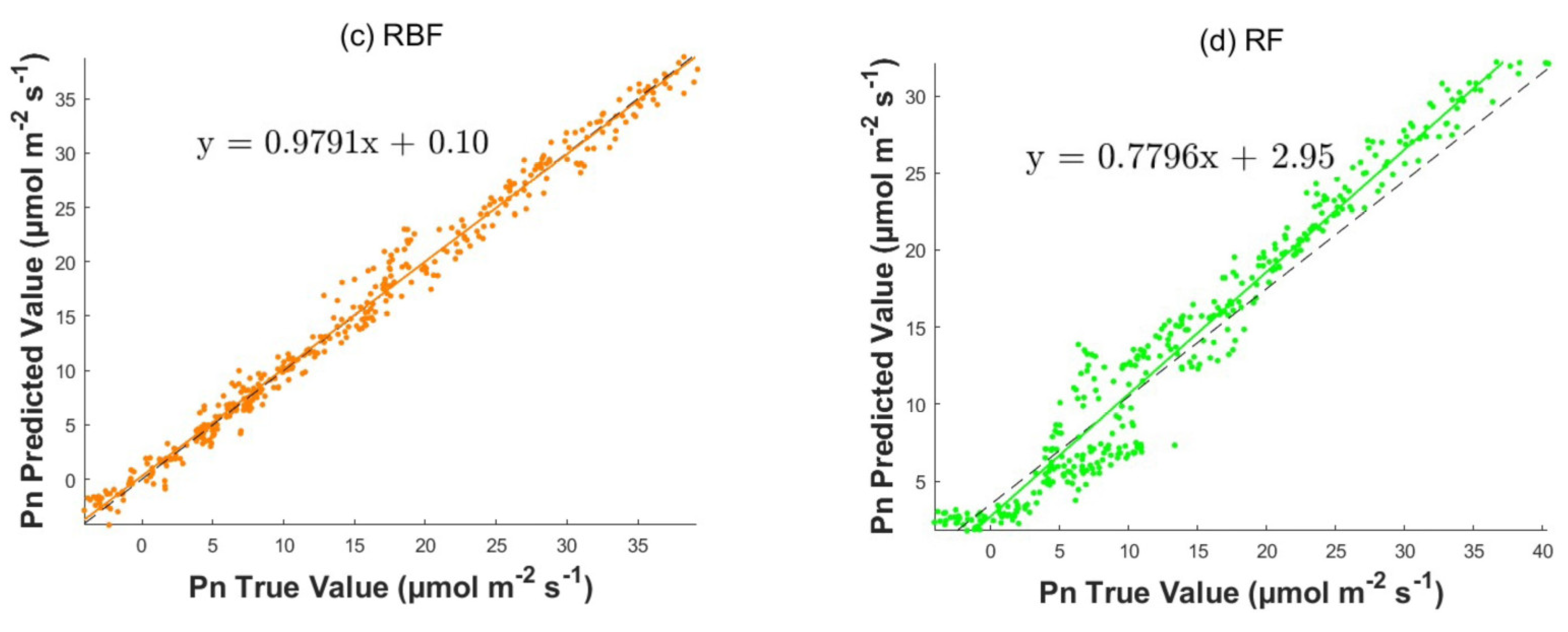
3.2.2. Comparative Analysis of Prediction Models

In this study, the performance of the SVR algorithm, BP neural network, RBF neural network, and RF algorithm were compared to validate the performance of photosynthesis rate models constructed by different modeling approaches. The evaluation results of the training and test sets were presented in

Table 1. Performance comparison of Pn prediction models using SVR, BP, RBF, and RF algorithms on the training dataset.

Regression Algorithm	R2	RMSE (μmol m−2 s−1)	MAE (μmol m−2 s−1)	MBE (μmol m−2 s−1)	MAPE
SVR	0.9975	0.4897	0.3937	−0.0202	0.0717
BP	0.9899	1.0681	0.8108	0.0711	0.1321
RBF	0.9879	1.1857	0.8894	−0.0006	0.1376
RF	0.9428	2.6056	2.1055	−0.0059	0.5393

Using five evaluation metrics: coefficient of determination (R²), root mean square error (RMSE, μmol m⁻² s⁻¹), maximum absolute error (MAE, μmol m⁻² s⁻¹), mean bias error (MBE, μmol m⁻² s⁻¹), and mean absolute percentage error (MAPE).

and

Table 2. Validation of Pn prediction models on the testing dataset, comparing SVR, BP, RBF, and RF algorithms.

Regression Algorithm	R2	RMSE (μmol m−2 s−1)	MAE (μmol m−2 s−1)	MBE (μmol m−2 s−1)	MAPE
SVR	0.9941	0.6988	0.5166	−0.0375	0.0907
BP	0.9887	1.1977	0.9062	−0.0557	0.1309
RBF	0.9867	1.2739	0.9679	0.0098	0.1671
RF	0.9391	2.6522	2.1055	−0.2399	0.4405

Metrics include R², RMSE (μmol m⁻² s⁻¹), MAE (μmol m⁻² s⁻¹), MBE (μmol m⁻² s⁻¹), and MAPE.

, respectively. The SVR algorithm outperformed the other three algorithms in the training set with an R² of 0.9975, an RMSE of 0.4897 μmol m⁻² s⁻¹, an MAE of 0.3937 μmol m⁻² s⁻¹, an MBE of −0.0202 μmol m⁻² s⁻¹, and an MAPE of 0.0717 (Table 1). This result suggests that the SVR algorithm is advantageous in constructing photosynthetic rate prediction models because it can better predict the trend of photosynthetic rate during the fruiting period of chili peppers.

To further validate the prediction performance of the photosynthetic rate prediction model on unknown data, we calculated the evaluation indexes of each model from the test dataset. The SVR algorithm had an R² of 0.9941, an RMSE of 0.6988 μmol m⁻² s⁻¹, an MAE of 0.5166 μmol m⁻² s⁻¹, an MBE of −0.0375 μmol m⁻² s⁻¹, and an MAPE of 0.0907, which were superior to the other algorithms (Table 2). This further confirmed the accuracy of the SVR algorithm in constructing photosynthetic rate prediction models.

After the models were constructed, their generalization capabilities were evaluated on the test set. The models were used to calculate the Pn values for the test set, which were then compared with the measured Pn values. To visualize the comparison results, the predicted values were plotted against the measured values (Figure 4). The fitted slope of the predicted photosynthetic rate of the SVR model was 0.9927, the closest to 1, and the intercept was 0.07, the closest to 0. These results confirm that the Pn prediction model established using the SVR algorithm performs the best.

4. Discussion

In facility agriculture, environmental factors such as light intensity, CO₂ concentration, and temperature change significantly over time due to weather, seasonal, and daily cycles. These changes make it difficult for crops to maintain optimal growing conditions [37]. Therefore, understanding how these factors interact and collectively affect photosynthetic rates in chili peppers is essential for optimizing facility environmental conditions and maintaining optimal crop growth. During the fruiting period, photosynthesis in chili peppers is influenced by a combination of light intensity, CO₂ concentration, and temperature. Specifically, high light intensity can cause photoinhibition, low CO₂ concentration can reduce carboxylation efficiency, and high temperature can induce heat stress [38]. To elucidate these dynamics, we systematically investigated the coupled effects of these three major environmental factors on the Pn during the fruiting period of chili peppers.

The trend of Pn showed a nonlinear response with changes in temperature, CO₂ concentration and PPFD. When the temperature was lower than 20 °C, the Pn values were lower, which may be attributed to the inhibition of the activities of enzymes related to photosynthesis in this temperature range [13]. As the temperature increased, the Pn values also increased, reflecting the activation of these enzymes in the optimum temperature range [14]. However, Pn began to decrease when the temperature exceeded 30 °C, which may indicate the presence of high temperature stress, resulting in the inactivation of key enzymes such as RuBisCO [14]. Moreover, under each temperature–CO₂ concentration combination, Pn showed a rapid increase followed by stabilization with increasing PPFD. This phenomenon can be attributed to the fact that the driving forces at the initial stage were the increase in PSII photochemical efficiency (Fv/Fm), the acceleration of linear electron transfer rate, and the increase in ATP/NADPH synthesis, which promoted the regeneration of RuBP and the Calvin cycle [8,39]. When at higher levels of PPFD, the stabilization of Pn reflects a shift in biochemical metabolic limitation, where the maximum rate of carboxylation of RuBisCO and the ability to assimilate CO₂ become the main limiting factors [40]. Similarly, under each temperature–PPFD combination, the same trend was observed with respect to CO₂ concentration, with an initial rapid increase in Pn possibly due to the role of CO₂ as a substrate for RuBisCO [41]. The subsequent slowing down of the enhancement of Pn suggests that the activity or regenerative capacity of RuBisCO is limited and that the rate of regeneration of RuBP and the availability of chloroplast ATP/NADPH become new limiting factors [42]. These findings provide key thresholds for optimizing environmental conditions in protected horticulture, allowing precise control to maximize photosynthetic efficiency.

The photosynthetic rate prediction model constructed using the SVR algorithm outperforms the other three regression algorithms on both the training and test sets. This superiority may be attributed to the fact that SVR transforms nonlinear problems into linearly separable problems in high-dimensional space through kernel function mapping, and its structural risk-minimization principle effectively balances the model complexity and generalization capability [26]. In contrast, BP and RBF neural networks rely on the empirical risk minimization principle and are therefore weak in modeling complex nonlinear relationships. Although the RF model reduces the risk of overfitting through bootstrap sampling and feature selection, its inherent tree-based nature results in a step effect when predicting continuous variables. In this study, there were less than 2000 data points and the input data were three-dimensional, so the neural network algorithm may be more suitable for large samples with a large number of inputs [43]. The data set used here is not sufficient to learn the optimal relationship between output and input before convergence. On the other hand, the SVR algorithm can compute the optimal hyperplane that fits the data, demonstrating stronger modeling capabilities for the complex nonlinear relationships among environmental factors (light intensity, CO₂ concentration, and temperature) in photosynthesis. This advantage is especially prominent under small sample conditions [44]. Therefore, the SVR algorithm may be more appropriate for small sample sets such as the one used in this study.

Although the SVR-based model had strong predictive performance, it was limited to predicting short-term (minute-scale) Pn under steady-state conditions, and its application to long-term crop growth optimization requires further consideration. Specifically, maximizing instantaneous Pn may not translate linearly into increased biomass accumulation or fruit yield, especially under extended photoperiods or extreme environmental conditions. This situation may trigger source–sink imbalances [45]. To address this limitation, future research could consider the development of environmental optimization models at multiple time scales by incorporating source–sink regulation mechanisms. This integrated approach will balance short-term photosynthetic efficiency with long-term growth performance, especially under prolonged light or extreme environmental parameters.

In addition, the findings of this study can be further translated into practical applications, such as the development of a facility-based environmental regulation system. This system could utilize real-time monitoring of environmental parameters (light intensity, CO₂ concentration, and temperature) combined with our SVR prediction model to rapidly and accurately estimate Pn values, providing decision-making support for dynamic environmental optimization in protected agriculture. Given the similarities in photosynthetic characteristics among different plant species, this approach is also applicable for predicting photosynthetic rates in other crops, demonstrating broad application potential.

5. Conclusions

An SVR model was shown to effectively capture the complex, nonlinear interactions among light intensity, CO₂ concentration, and temperature that determine chili pepper photosynthesis during fruiting. By accurately predicting the Pn from these environmental inputs, the SVR approach provided a reliable framework even with limited, high-dimensional data. The results highlight how these variables jointly influence photosynthetic efficiency and identify optimal conditions that can guide precision agriculture practices. In sum, this work deepens our mechanistic understanding of multi-factor control of photosynthesis and offers a practical predictive tool for optimizing growth in controlled-environment agriculture.

References

1. Hernández-Morales, C.A.; Luna-Rivera, J.; Perez-Jimenez, R.J.C.C. Design and deployment of a practical IoT-based monitoring system for protected cultivations. Comput. Commun. 2022, 186, 51–64. [Google Scholar] [CrossRef]
2. Xu, Y.; Li, J.; Wan, J.J.T.C.J. Agriculture and crop science in China: Innovation and sustainability. Crop J. 2017, 5, 95–99. [Google Scholar] [CrossRef]
3. Wang, H.; Meng, X.Y.; Chen, Z.R.; Zhang, X.H.; Cheng, R.F.; Zhang, Y.; Li, W.; Song, W.X.; Zhang, Y. A feedback control method for plant factory environment based on photosynthetic rate prediction model. Comput. Electron. Agric. 2023, 211, 108007. [Google Scholar] [CrossRef]
4. Jamil, F.; Ibrahim, M.; Ullah, I.; Kim, S.; Kahng, H.K.; Kim, D.-H.J.C.; Agriculture, E.i. Optimal smart contract for autonomous greenhouse environment based on IoT blockchain network in agriculture. Comput. Electron. Agric. 2022, 192, 106573. [Google Scholar] [CrossRef]
5. Jo, W.J.; Shin, J.H. Development of a transpiration model for precise tomato (Solanum lycopersicum L.) irrigation control under various environmental conditions in greenhouse. Plant Physiol. Biochem. 2021, 162, 388–394. [Google Scholar] [CrossRef]
6. Xin, P.P.; Zhang, H.H.; Hu, J.; Shao, Z.C.; Peters, R.T. CO2 control system design based on optimized regulation model. Appl. Eng. Agric. 2019, 35, 377–388. [Google Scholar] [CrossRef]
7. Smith, E.N.; van Aalst, M.; Tosens, T.; Niinemets, Ü.; Stich, B.; Morosinotto, T.; Alboresi, A.; Erb, T.J.; Gómez-Coronado, P.A.; Tolleter, D.J.M. Improving photosynthetic efficiency toward food security: Strategies, advances, and perspectives. Mol. Plant 2023, 16, 1547–1563. [Google Scholar] [CrossRef]
8. Gao, P.; Lu, M.; Yang, Y.; Li, H.; Tian, S.; Hu, J.J.C.; Agriculture, E.I. A predictive model of photosynthetic rates for eggplants: Integrating physiological and environmental parameters. Comput. Electron. Agric. 2025, 234, 110241. [Google Scholar] [CrossRef]
9. Niu, Y.; Lyu, H.; Liu, X.; Zhang, M.; Li, H. Photosynthesis prediction and light spectra optimization of greenhouse tomato based on response of red–blue ratio. Sci. Hortic. 2023, 318, 112065. [Google Scholar] [CrossRef]
10. Chen, D.Y.; Zhang, J.H.; Zhang, Z.X.; Lu, Y.Q.; Zhang, H.H.; Hu, J. A high efficiency CO2 concentration interval optimization method for lettuce growth. Sci. Total Environ. 2023, 879, 162731. [Google Scholar] [CrossRef]
11. Pan, T.; Wang, Y.; Wang, L.; Ding, J.; Cao, Y.; Qin, G.; Yan, L.; Xi, L.; Zhang, J.; Zou, Z. Increased CO2 and light intensity regulate growth and leaf gas exchange in tomato. Physiol. Plant. 2020, 168, 694–708. [Google Scholar] [CrossRef]
12. Orujova, T.Y.; Bayramov, S.M.; Gurbanova, U.A.; Babayev, H.G.; Aliyeva, M.N.; Guliyev, N.M.; Feyziyev, Y.M. Diurnal temperature-related variations in photosynthetic enzyme activities of two C4 species of Chenopodiaceae grown in natural environment. Photosynthetica 2018, 56, 1107–1112. [Google Scholar] [CrossRef]
13. Dickinson, K.E.; Lalonde, C.G.; McGinn, P.J. Effects of spectral light quality and carbon dioxide on the physiology of Micractinium inermum: Growth, photosynthesis, and biochemical composition. J. Appl. Phycol. 2019, 31, 3385–3396. [Google Scholar] [CrossRef]
14. Galmés, J.; Capó-Bauçà, S.; Niinemets, Ü.; Iñiguez, C. Potential improvement of photosynthetic CO2 assimilation in crops by exploiting the natural variation in the temperature response of Rubisco catalytic traits. Curr. Opin. Plant Biol. 2019, 49, 60–67. [Google Scholar] [CrossRef] [PubMed]
15. Gao, P.; Lu, M.; Xu, J.H.; Zhang, H.M.; Li, Y.F.; Hu, J. IPECM Platform: An open-source software for greenhouse environment regulation using machine learning and optimization algorithm. Comput. Electron. Agric. 2024, 217, 108564. [Google Scholar] [CrossRef]
16. Ye, Z.P.; Duan, S.H.; Chen, X.M.; Duan, H.L.; Gao, C.P.; Kang, H.J.; An, T.; Zhou, S.X. Quantifying light response of photosynthesis: Addressing the long-standing limitations of non-rectangular hyperbolic model. Photosynthetica 2021, 59, 185–191. [Google Scholar] [CrossRef]
17. Yin, X.; Busch, F.A.; Struik, P.C.; Sharkey, T.D. Evolution of a biochemical model of steady-state photosynthesis. Plant Cell Environ. 2021, 44, 2811–2837. [Google Scholar] [CrossRef]
18. Gao, P.; Tian, Z.W.; Lu, Y.Q.; Lu, M.; Zhang, H.H.; Wu, H.R.; Hu, J. A decision-making model for light environment control of tomato seedlings aiming at the knee point of light-response curves. Comput. Electron. Agric. 2022, 198, 107103. [Google Scholar] [CrossRef]
19. Filippi, P.; Jones, E.J.; Wimalathunge, N.S.; Somarathna, P.D.S.N.; Pozza, L.E.; Ugbaje, S.U.; Jephcott, T.G.; Paterson, S.E.; Whelan, B.M.; Bishop, T.F.A. An approach to forecast grain crop yield using multi-layered, multi-farm data sets and machine learning. Precis. Agric. 2019, 20, 1015–1029. [Google Scholar] [CrossRef]
20. Xin, P.P.; Zhang, H.H.; Hu, J.; Wang, Z.Y.; Zhang, Z.; Tao, Y.R. An Improved Photosynthesis Prediction Model Based on Artificial Neural Networks Intended for Cucumber Growth Control. Appl. Eng. Agric. 2018, 34, 769–788. [Google Scholar] [CrossRef]
21. Hu, J.; Xin, P.P.; Zhang, S.W.; Zhang, H.H.; He, D.J. Model for tomato photosynthetic rate based on neural network with genetic algorithm. Int. J. Agric. Biol. Eng. 2019, 12, 179–185. [Google Scholar] [CrossRef]
22. Kmet, T.; Kmetova, M.J.I.S. Adaptive critic design and Hopfield neural network based simulation of time delayed photosynthetic production and prey–predator model. Inf. Sci. 2015, 294, 586–599. [Google Scholar] [CrossRef]
23. Santos, C.E.D.; Sampaio, R.C.; Coelho, L.D.; Bestard, G.A.; Llanos, C.H. Multi-objective adaptive differential evolution for SVM/SVR hyperparameters selection. Pattern Recognit. 2021, 110, 107649. [Google Scholar] [CrossRef]
24. Sun, Y.T.; Ding, S.F.; Zhang, Z.C.; Jia, W.K. An improved grid search algorithm to optimize SVR for prediction. Soft Comput. 2021, 25, 5633–5644. [Google Scholar] [CrossRef]
25. Abdollahpour, S.; Kosari-Moghaddam, A.; Bannayan, M.J.I.P.i.A. Prediction of wheat moisture content at harvest time through ANN and SVR modeling techniques. Inf. Process. Agric. 2020, 7, 500–510. [Google Scholar] [CrossRef]
26. Xin, P.P.; Li, B.; Zhang, H.H.; Hui, J. Optimization and control of the light environment for greenhouse crop production. Sci. Rep. 2019, 9, 8650. [Google Scholar] [CrossRef]
27. Lu, M.; Gao, P.; Li, H.M.; Sun, Z.T.; Yang, N.; Hu, J. An optimization approach for environmental control using quantum genetic algorithm and support vector regression. Comput. Electron. Agric. 2023, 215, 108432. [Google Scholar] [CrossRef]
28. Mohammadi, B.; Mehdizadeh, S. Modeling daily reference evapotranspiration via a novel approach based on support vector regression coupled with whale optimization algorithm. Agric. Water Manag. 2020, 237, 106145. [Google Scholar] [CrossRef]
29. Wei, Z.C.; Wan, X.B.; Lei, W.Y.; Yuan, K.K.; Lu, M.; Li, B.; Gao, P.; Wu, H.R.; Hu, J. A Cucumber Photosynthetic Rate Prediction Model in Whole Growth Period with Time Parameters. Agriculture 2023, 13, 204. [Google Scholar] [CrossRef]
30. Hou, Z.; Niu, J.; Zhu, J.; Lu, L. Flow Prediction of a Measurement and Control Gate Based on an Optimized Back Propagation Neural Network. Appl. Sci. 2023, 13, 12313. [Google Scholar] [CrossRef]
31. Pu, L.R.; Li, Y.F.; Gao, P.; Zhang, H.H.; Hu, J. A photosynthetic rate prediction model using improved RBF neural network. Sci. Rep. 2022, 12, 9563. [Google Scholar] [CrossRef] [PubMed]
32. Li, J.H.; Zhu, D.S.; Li, C.X. Comparative analysis of BPNN, SVR, LSTM, Random Forest, and LSTM-SVR for conditional simulation of non-Gaussian measured fluctuating wind pressures. Mech. Syst. Signal Process. 2022, 178, 109285. [Google Scholar] [CrossRef]
33. Lin, L.; Liu, X.J.C.; Agriculture, E.i. Mixture-based weight learning improves the random forest method for hyperspectral estimation of soil total nitrogen. Comput. Electron. Agric. 2022, 192, 106634. [Google Scholar] [CrossRef]
34. Niu, Y.Y.; Lyu, H.H.; Liu, X.Y.; Zhang, M.; Li, H. Effects of supplemental lighting duration and matrix moisture on net photosynthetic rate of tomato plants under solar greenhouse in winter. Comput. Electron. Agric. 2022, 198, 107102. [Google Scholar] [CrossRef]
35. Hou, J.; Li, Y.; Sun, Z.; Wang, H.; Lu, M.; Hu, J.; Wu, H. A cooperative regulation method for greenhouse soil moisture and light using Gaussian curvature and machine learning algorithms. Comput. Electron. Agric. 2023, 215, 108452. [Google Scholar] [CrossRef]
36. Jiang, Q.; Zhu, L.; Shu, C.; Sekar, V. An efficient multilayer RBF neural network and its application to regression problems. Neural Comput. Appl. 2022, 34, 4133–4150. [Google Scholar] [CrossRef]
37. Niu, G.; Masabni, J.J.H. Plant production in controlled environments. Horticulturae 2018, 4, 28. [Google Scholar] [CrossRef]
38. Santosh, D.; Tiwari, K.; Singh, V.K.; Reddy, A.R.G.; Sciences, A. Micro climate control in greenhouse. Int. J. Curr. Microbiol. Appl. Sci. 2017, 6, 1730–1742. [Google Scholar] [CrossRef]
39. Kang, J.; Chu, Y.; Ma, G.; Zhang, Y.; Zhang, X.; Wang, M.; Lu, H.; Wang, L.; Kang, G.; Ma, D.J.T.C.J. Physiological mechanisms underlying reduced photosynthesis in wheat leaves grown in the field under conditions of nitrogen and water deficiency. Crop J. 2023, 11, 638–650. [Google Scholar] [CrossRef]
40. Shi, Y.; Ke, X.; Yang, X.; Liu, Y.; Hou, X. Plants response to light stress. J. Genet. Genom. 2022, 49, 735–747. [Google Scholar] [CrossRef]
41. Fukayama, H.; Mizumoto, A.; Ueguchi, C.; Katsunuma, J.; Morita, R.; Sasayama, D.; Hatanaka, T.; Azuma, T. Expression level of Rubisco activase negatively correlates with Rubisco content in transgenic rice. Photosynth. Res. 2018, 137, 465–474. [Google Scholar] [CrossRef] [PubMed]
42. Pang, Y.; Liao, Q.; Peng, H.; Qian, C.; Wang, F.J.P. CO2 mesophyll conductance regulated by light: A review. Planta 2023, 258, 11. [Google Scholar] [CrossRef] [PubMed]
43. van de Ven, G.M.; Siegelmann, H.T.; Tolias, A.S. Brain-inspired replay for continual learning with artificial neural networks. Nat. Commun. 2020, 11, 4069. [Google Scholar] [CrossRef] [PubMed]
44. Chen, X.Y.; Jiang, Z.H.; Tai, Q.L.; Shen, C.S.; Rao, Y.; Zhang, W. Construction of a photosynthetic rate prediction model for greenhouse strawberries with distributed regulation of light environment. Math. Biosci. Eng. 2022, 19, 12774–12791. [Google Scholar] [CrossRef]
45. Vincenzi, E.; Ji, Y.; Kerstens, T.; Lai, X.; Deelen, S.; de Beer, E.; Millenaar, F.; Marcelis, L.F.; Heuvelink, E.J.S.H. Duration, not timing during the photoperiod, of far-red application determines the yield increase in tomato. Sci. Hortic. 2024, 338, 113553. [Google Scholar] [CrossRef]
Figure 1. Flowchart of constructing photosynthetic rate prediction model using SVR algorithm.
Horticulturae 11 00502 g001
Figure 2. Effects of different temperatures, CO2 concentrations, and PPFD on the Pn of pepper leaves (Pn: represented by a color scale) Note: The color scale indicates the magnitude of the Pn (μmol m−2 s−1), with a gradient from cool colors (e.g., blue, low Pn) to warm colors (e.g., red, high Pn). The figure highlights the optimal conditions for maximum Pn (39.2 μmol m−2 s−1) at PPFD = 1800 μmol m−2 s−1, CO2 concentration = 1600 μmol mol−1, and temperature = 30 °C.
Horticulturae 11 00502 g002
Figure 3. Comparison between SVR model predictions (colored surfaces) and measured Pn values (red dots) at different temperature conditions. (a): 12 °C; (b): 15 °C; (c): 20 °C (d): 22 °C; (e): 24 °C; (f): 26 °C (g): 28 °C (h): 30 °C; (i): 32 °C; (j): 35 °C. The color gradient of prediction surfaces represents Pn magnitude (−5 to 40 μmol m−2 s−1).
Horticulturae 11 00502 g003aHorticulturae 11 00502 g003b
Figure 4. Comparison of predicted Pn values with measured Pn values on the test set for four algorithms: (a) SVR algorithm, (b) BP neural network, (c) RBF neural network, and (d) RF algorithm. The black dashed line indicates the ideal 1:1 relationship, and the solid line indicates the linear regression fitting results.
Horticulturae 11 00502 g004aHorticulturae 11 00502 g004b