Article

Evapotranspiration-Based Irrigation Management Effects on Yield and Water Productivity of Summer Cauliflower on the California Central Coast

1
Cooperative Extension, Monterey County, Division of Agriculture and Natural Resources, University of California, 1432 Abbott St., Salinas, CA 93901, USA
2
Department Applied Environmental Science, California State University Monterey Bay, Seaside, CA 93955, USA
3
Earth Science Division, NASA Ames Research Center, Moffett Field, CA 94035, USA
4
Crop Improvement and Protection Research Unit, USDA Agricultural Research Service, Salinas, CA 93905, USA
*
Author to whom correspondence should be addressed.
Horticulturae 2025, 11(3), 322; https://doi.org/10.3390/horticulturae11030322
Submission received: 20 December 2024 / Revised: 23 February 2025 / Accepted: 24 February 2025 / Published: 15 March 2025
(This article belongs to the Special Issue Advancements in Horticultural Irrigation Water Management)

Abstract

:
Improvements in irrigation water productivity constitute an ongoing effort globally. In California, growers are under regulatory pressure to stabilize groundwater levels and reduce nitrate leaching, partially, by further improvements in irrigation optimization. Evapotranspiration (ET)-based methods can inform crop water requirements and boost irrigation efficiency, but in practice, they can be challenging for farmers to implement, especially in vegetable systems. Irrigation field trials were conducted near Salinas CA in 2018 and 2019 to evaluate the crop coefficient model employed by the CropManage ET-based irrigation decision support system (DSS) for summer cauliflower (Brassica oleracea var. botrytis cv. Symphony) and investigate potential water savings through improved irrigation scheduling. Overhead sprinklers were used for crop establishment, and surface drip was used subsequently. A randomized complete block design was used to administer treatments near 50, 75, 100, and 150% of crop evapotranspiration (ET) during the drip period with an added treatment at 125% in 2019. Water requirement for the 100% treatment was determined by the CropManage DSS model based on crop coefficients derived from fractional canopy cover. Deliveries to remaining treatments were scaled proportionally. The total yield and irrigation productivity were maximized by the 100% treatment both years with total applied water ranging from 275 to 300 mm. At present, the reported water application for summer cauliflower averages 465 mm in the region. Hence, implementing ET-based irrigation scheduling, administered through the CropManage DSS, could reduce water use in summer cauliflower by an average of 30% relative to current practices and serve to enhance groundwater management while maintaining crop returns.

1. Introduction

The Central Coast of California is a main production region of cool season vegetables in the United States. The region has a mild Mediterranean climate with minimal rainfall during the production period from late March through October. Cool-season vegetables generally require an ample supply of water to minimize or avoid crop stress, meet market quality standards, and attain economically viable yields. Consequently, growers in this region rely on groundwater to irrigate their crops.
California’s Sustainable Groundwater Management Act requires agricultural producers to improve the balance of groundwater pumping and recharge in most basins statewide, affecting 88% of irrigated lands (2.7 million hectares). Central Coast basins are considered medium-to-high priority, thus requiring the development of a groundwater sustainability plan, with certain aquifers deemed critically overdrafted. In addition, regional vegetable and other specialty crop producers are under regulatory pressure to reduce groundwater nitrate, which partially results from use of nitrogen fertilizer and subsequent leaching of nitrate during irrigations [1,2]. Overdraft is also linked with seawater intrusion into coastal aquifers [3]. Effective irrigation practice can benefit groundwater quality by reducing nitrate loads [4] and mitigating seawater intrusion [5].
Cauliflower is one of the economically important cool season vegetables produced on the Central Coast. California produces about 90% of the U.S. cauliflower supply. The crop is grown in several parts of the state during various times of year [6], but the Central Coast region accounts for about one half of statewide cauliflower production, with associated crop value exceeding USD 200 million annually [7,8].
Despite having a high economic value, few studies have been performed on cauliflower water relations in the Salinas Valley, which is the main Central Coast production zone. The FAO-56 crop coefficient guidelines for cauliflower [9], for instance, derive from fall/winter crop on a 140-day growing season in the California desert. As part of a broader update of FAO-56 methods, a comprehensive review by Pereira et al. [10] cited an overall lack of research on cauliflower crop coefficients. It is recognized that horticultural crop coefficients in general are sensitive to differences in such aspects as cultural practice, cultivar, and planting time [11], and regional characterization is recommended.
Studies in various production regions across the globe have examined cauliflower water requirements [12,13], optimal irrigation methods [14,15], relationships of irrigation volume with yield and water use efficiency [16,17,18], and water–nutrient interactions [19,20,21,22].
Prior monitoring of cole crops (Brassicas) on the California Central Coast, including cauliflower, revealed that applied water can range up to 200% of estimated crop ET [23]. Under these conditions, high transpiration rates are maintained by limiting soil moisture depletion between irrigations. Overhead sprinklers are typically used with irrigation events usually occurring weekly after crop establishment. Recent observation suggests that an increasing number of cauliflower plantings in the region undergo conversion to drip irrigation following crop establishment, which is a practice that can increase irrigation efficiency in vegetables [24] and improve access for field operations including harvest [6]. Total applied water typically ranges from 610 to 914 mm for Central Coast summer cauliflower under sprinkler irrigation [6]. A more recent industry survey of cauliflower conducted by the Central Coast Regional Water Quality Control Board of 788 Central Coast farms, which included crops grown throughout the year by various irrigation systems, indicated a range of 127–1016 mm of applied water with an average of 465 mm.
Despite documented overdraft of groundwater supplies and data indicating an over-application of irrigation water to cauliflower, few tools have been widely adopted to improve irrigation scheduling to date. Cahn and Johnson [25] reviewed some of the operational challenges facing medium to large vegetable farms in California regarding water management efficiency. A main challenge is the concurrent management of many individual fields. For instance, a large operation in the Salinas Valley may farm up to 2000 ha of vegetables annually with average planting size near 4 ha. A diverse operation may produce up to 30 types of vegetables with varying water and nutrient requirements. Fields typically present a range of site-specific attributes with respect to soil texture, cultural practice, and microclimate. Irrigations must be coordinated with other farming activities such as weed control, fertilizer management, and pesticide applications to accommodate tractor or field-crew access. An added complication is the customary use of different water delivery methods (sprinkler, drip, flood) based on such considerations as crop type, planting density, and development stage.
The installation of soil moisture sensors is uncommon in vegetable fields in the Salinas Valley due to short growing periods, frequent tractor cultivation, and labor needed for installation and removal [25]. The implementation of irrigation schedules based on evapotranspiration data also has been limited due to effort required to calculate irrigation runtimes for each planting and difficulty in calculating daily crop coefficients from FAO-56 or other published sources for multiple plantings at various stages of maturity. Consequently, many farm managers tend to follow predetermined irrigation schedules to simplify water management and make small ongoing adjustments based on observations of the crop, soil, and weather conditions.
The CropManage (CM) web application was developed to assist growers with evapotranspiration (ET)-based irrigation scheduling [25,26]. CM combines transpiration and soil evaporation crop coefficients with reference ET to develop irrigation schedules meeting daily crop water requirements. Since its original development in lettuce, the model has been tested and expanded to address additional cool-season vegetables [27,28,29]. Irrigation recommendations assume that the crop is well watered to avoid stress and plants are otherwise healthy.
The main goal of this study was to evaluate an ET-based irrigation scheduling model in cauliflower and estimate potential water savings through field trials examining the interaction of applied water with response variables related to yield and water productivity. In addition to providing information on key water relations in the Salinas Valley, the study served to test and refine CM for on-farm management of cauliflower and to improve knowledge of cool season vegetable crop coefficients.

2. Materials and Methods

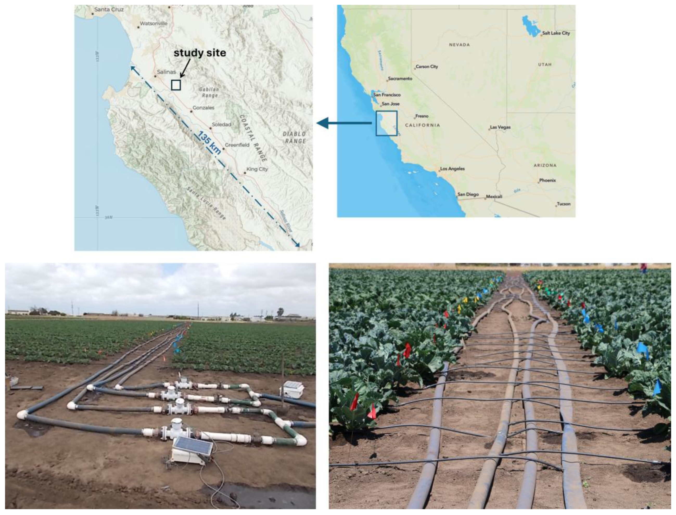
2.1. Field Experiment

Replicated field trials in cauliflower (cv. Symphony) were performed during 2018 and 2019 on Chualar sandy loam soil at the USDA Agricultural Field Station near Salinas, CS, USA (36.626° N, 121.542° W) (Figure 1). Groundwater with an average electrical conductivity of 0.53 dSm−1, pH of 7.4, and containing 6 ppm NO3-N, was used for all irrigations. Seedlings were mechanically transplanted 27 cm apart into single rows on 1 m wide raised beds. Transplant dates for the two experiments were 2 May 2018 and 30 April 2019. Overhead sprinklers were used to apply 60–71 mm of water to establish the transplants during the first two weeks of the crop. An additional 35 mm of precipitation occurred during transplant establishment in 2019. Precipitation was negligible in 2018. Experimental irrigation treatments were then imposed by drip irrigation. New medium-flow (emitter discharge 0.55 L hr−1, emitter spacing 20 cm) drip tape was used for each trial. The drip tape was placed on the soil surface adjacent to the plant rows. A distribution uniformity of 90% was assumed for both years based upon the tape manufacturer’s coefficient of variation in the emitter discharge rates, and previous evaluations of emitter discharge uniformity made for new drip tape installed in Salinas Valley vegetable fields (Cahn, unpublished data).
Standard production practices for the region were followed. Uniform amounts of pesticide, nitrogen (20 kg ha−1 preplant, 336 kg ha−1 by fertigation), and phosphorus (67 kg ha−1 preplant) were applied across treatments and years. Potassium totals were 118 kg ha−1 across treatments in 2018 and 162 kg ha−1 in 2019. No crop development limitations were observed with respect to variation in soil fertility, soil salinity, plant population, insect pests, or disease.

2.2. Irrigation Treatments

ET-based irrigation treatments were guided by a provisional version of CropManage [30]. Irrigation treatments nominally represented 50, 75, 100 and 150% (T50, T75, T100, T150) of crop ET during the drip phase. In 2019, a new treatment at 125% of crop ET (T125) was introduced to further investigate the possible value of applying additional water to maintain crop quality. T100 corresponded to the CropManage recommended irrigation volume. The additional treatments served to evaluate the model and test the hypothesis that commercial production and irrigation water productivity can be maximized under the T100 treatment. The T150 treatment corresponded to a water volume more typically applied by commercial growers, thereby providing a comparison of potential water savings that might be realized through ET-based scheduling using tools like CM.
Treatments were assigned to plots following a randomized complete block design with six replicated plots per treatment. Individual plots measured 41 m by six beds in 2018 and 41 m by five beds in 2019. Drip irrigation was applied 2–3 times per week. An irrigation manifold equipped with digital flowmeters (Model AG3000, Seametrics, Kent, WA, USA) was used to control water applications on each treatment (Figure 1).

2.3. ETc Model

CropManage was used to prescribe the full water requirement, represented by T100, per irrigation event. Proportional scaling factors (0.5, 0.75, 1.25, 1.5) were applied to the T100 volume to define irrigation targets for the remaining treatments.
Crop evapotranspiration (ETc) and associated water requirements can be evaluated largely in terms of canopy fractional cover (Fc), crop coefficients (Kc), and soil evaporation coefficients (Ke) [9,31,32,33,34]. Daily Fc, based on typical crop development for the region as a function of days after planting, is the main basis for deriving daily Kc and ETc. CM updates for these variables daily throughout the growth cycle pursuant to various inputs including planting and expected harvest dates, bed configuration, expected maximum Fc, soil texture, precipitation, irrigation method, distribution uniformity, and water application rate. An option enables the ingestion of Fc ground data or observations from NASA’s Satellite Irrigation Management Support [34,35] to adjust the default Fc curve as needed to more closely reflect actual field development.
A phenology curve relating canopy fractional cover (Fc) to crop cycle fraction was developed from prior measurements in commercial fields (Cahn, unpublished data) (Figure 2A). A transpiration coefficient (T), also commonly referred to as basal crop coefficient (Kcb), was then derived from Fc after findings of Gallardo et al. [36] (Figure 2B). The coefficient expresses daily water use as a proportion of grass reference ET (ETo) from the California Irrigation Management Information System (CIMIS), as derived by the Penman–Monteith equation [37,38]. The T coefficient reaches a maximum of 1.05 when Fc reaches 0.9. An evaporation coefficient (Ke) accounted for vaporization from exposed soil after irrigation and precipitation events. For this study, Ke was assigned a set value based on the number of days since wetting. The initial value (day 0) was estimated by the fraction of the field wetted during an irrigation or rain event. Ke values for subsequent days were empirically estimated as described by Gallardo et al. [39], using volumetric soil moisture measurements of undisturbed cores collected from the 0–15 cm depth at 24-hour intervals in vegetable fields near the trial site during crop germination (Cahn, unpublished data). For sprinkler irrigation and rainfall, Ke was set to 1.0 on day 0, 0.4 on day 1, 0.05 on day 2, and zero thereafter. For drip irrigation, which wets only about 30% of the soil surface, Ke was set to 0.3 on day 0, 0.1 on day 1, 0.05 on day 2, and zero thereafter. Daily ETc was then derived by multiplying the greater of T or Ke by ETo as monitored by CIMIS station #214, which was located within 1 km of the field trial. For a given irrigation event, CM calculated the cumulative ETc for days since the last event. An irrigation recommendation accounting for rainfall and distribution uniformity was then issued in terms of water depth and system run time based on application rate. Additional detail on CM computation is provided by Johnson et al. [27] and Cahn et al. [40,41].

2.4. Field Measurements

Soil samples from the root zone of the crop were periodically collected and analyzed for nitrate using quick test strips (Mquant, Merck, Darmstadt, Germany) [42] to guide fertigation activity. A boom-mounted multispectral camera (Rebel T5i 700D, Canon Inc., Melville, NY, USA) was used to periodically monitor Fc to verify the CM phenology curve. As an additional check on CM operation, tensiometers (Model SR, Irrometer, Riverside, CA, USA) installed in the root zone at approximately 35 cm depth, were used to monitor soil water potential immediately before mid- to late-season irrigation events. These depths were similar to those of Thompson et al. [20] for drip-irrigated cauliflower.
Harvest zones measuring 15 m in length for four central beds in 2018 and three central beds in 2019 were established in each plot. Two fresh-product harvest passes were conducted per trial (68 and 71 days after transplanting (DAT) in 2018, 70 and 73 DAT in 2019). During the first pass, a professional cutting crew was instructed to concentrate effort on heads of marketable size (suitable for standard 9- or 12-count packing cartons) regardless of any visually apparent blemish or defect. During the second pass, the crew removed all remaining marketable size heads again without regard to defect. The heads were immediately weighed to determine total yield, which was the main response variable of interest to this study. All harvested heads were visually inspected for quality defects [43], divided into marketable and cull categories, and reweighed. Culls were segregated and weighed, and marketable yield was derived as the difference between total yield and cull yield. In addition, a random sample of 30 marketable heads per plot was evaluated for size distribution based on weight during both 2019 harvest passes. The following thresholds were applied: 0.7–1.05 kg were classified as small (suitable for 16 ct. cartons), 1.05–1.4 kg as medium (12 ct.), and 1.4–2.0 kg as large (9 ct). Oversize heads (>2 kg) were considered non-marketable as fresh product.
The aboveground biomass yield was evaluated 70 DAT in 2018 and 72 DAT in 2019 in areas adjacent to the harvest zones. Biomass harvest zones measured 3 m in length by two beds per plot. All plants were cut at soil level and immediately weighed. Heads and vegetation were separated and weighed to determine the relative contribution of each component. Fresh head and vegetation subsamples (~1 kg) were weighed, oven-dried dried for 48 h at 60 °C, re-weighed to determine water content, and then ground and analyzed for nitrogen content by the combustion method [44].

2.5. Water Productivity, N Uptake, and Statistical Analysis

Irrigation water productivity was calculated with respect to total head yield, fresh and dry aboveground biomass. In all cases, productivity was calculated in terms of production (kg) per unit (m3) of applied water.
Crop N uptake (kg ha−1) was calculated as the product of plant tissue N concentration and dry biomass yield. Fertilizer recovery (%) was calculated as N uptake divided by total applied N fertilizer.
The general linear means procedures of the SAS/STAT software, Version 9.4 of the SAS System for Windows 10 (SAS Institute, Inc., Cary, NC, USA), were used to statistically evaluate yield differences among irrigation treatments. The main effects of year and irrigation treatment, as well as their interaction, were evaluated at the p < 0.05 level for treatments common to both years (T50, T75, T100, and T150). In cases of significant interaction, the treatment means were presented by year and include the T125 treatment for 2019 trial. When treatment × year interaction was not significant, means were calculated from data combined from both years. Multiple means comparisons were performed when main effects were found to be statistically significant using a two-tailed protected Fisher’s test (p < 0.05).

3. Results

3.1. Applied Water Volumes and Soil Moisture Tension

Applied water ranged from 199 to 410 mm across treatments in 2018 and 179 to 369 mm in 2019 (Table 1). Precipitation was negligible in 2018, and was approximately 35 mm in 2019, mostly occurring during establishment. For reference, the median applied water volume reported by regional growers to the CCRWQCB in 2017 was 440 mm for cauliflower, which exceeded the total amount applied in the highest water treatment (T150).
Irrigation treatments showed a strong effect on soil moisture tension (Figure 3). During 2018, tensions were greatest in T50 and T75 throughout the measurement period (40–52 DAT), which was followed by T100. By 48 DAT, all three treatments exceeded 60 kPa. Similarly, in 2019, T75 had the highest tensions throughout the measurement period (48–62 DAT), which was followed by T100 (T50 was not measured in 2019). Both treatments reached values above 60 kPa by 54 DAT. In contrast, tensions in T150 (both years) and T125 (2019 only) generally remained below the 30 kPa maximum target suggested by the California cauliflower production guidelines [6] for the final month before harvest.

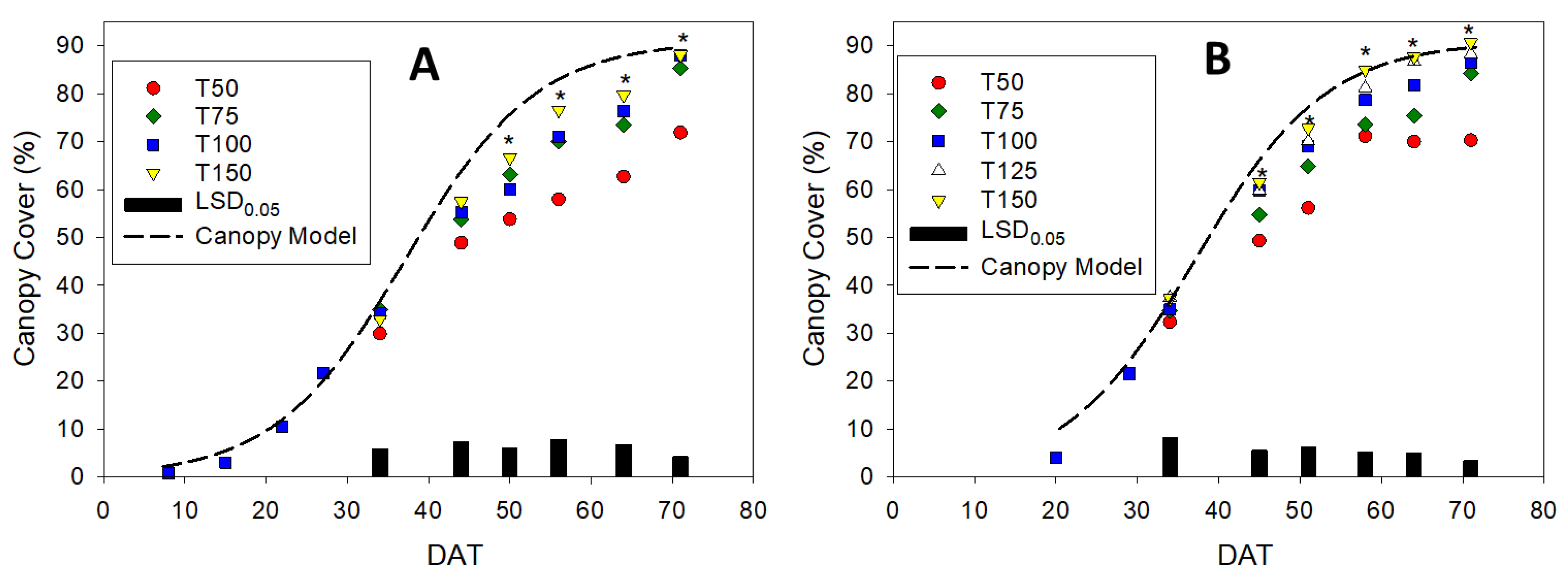
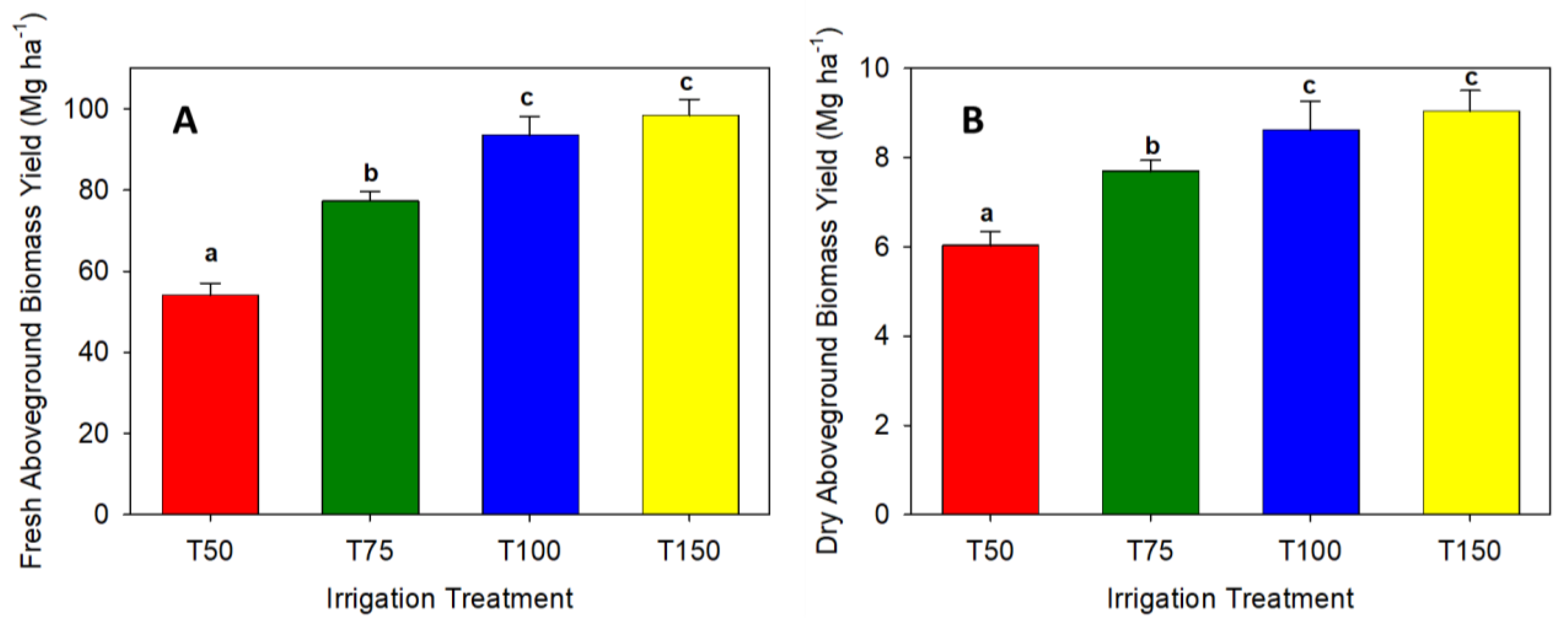
3.2. Treatment Effects on Crop Development and Yield

Plants in the T50 treatment had significantly less canopy development (Figure 4) after DAT 50 and 45 in 2018 and 2019, respectively, and were visibly stunted in size. Canopy cover of T50 was about 70% near harvest compared to 88% in T100 and T150. T75 had the next smallest canopy in 2019 and was significantly smaller than the higher water treatments on 58 and 64 DAT, but it was similar in size by 70 DAT. The main effects of irrigation treatment were statistically significant for most response variables measured at harvest. Also, many variables had statistically significant interactions between irrigation treatment and trial year. Irrigation treatments significantly affected the number of plants with marketable size heads, total yield of marketable size heads (total yield), and yield of heads of marketable size and quality (marketable yield). The incidence of plants with marketable size heads was highest for the T75–T150 treatments in 2018 (Table 2). In 2019, T100 and T125 had the highest number of plants with marketable sized heads. T150 had significantly fewer marketable size heads than the T100 and T75 treatments in 2019. It is possible that the higher applied water of this treatment delayed the development of the heads. The number of harvested heads was markedly lower for T50 compared to T100 in both years (17% lower in 2018, 45% lower in 2019) due to an abundance of unacceptably small heads.
In addition to affecting the number of marketable size heads, T50 produced smaller heads on average. Small size heads represented 63% of heads harvested from T50 compared to <30% of heads harvested from T100–T150. The percentage harvested as medium and large-sized heads was statistically similar for T100–T150, where medium size represented >50% of harvested heads, and large size represented 17% to 26% (Table 3). Medium heads generally have the highest market value.
Total yield ranged from 15.5 to 36.1 Mg ha−1 across treatments in both trials (Table 4). Total yields from T100 (32.2 Mg ha−1) and T150 (35.2 Mg ha−1) were not significantly different during 2018. The total yield of T150 (31.4 Mg ha−1) was statistically lower than T100 (36.1 Mg ha−1) and T125 (35.5 Mg ha−1) in 2019. For both years, the total yield from T75 was about 15% lower than that from T100 and T150, and the T50 yield was about 50% lower.
Marketable yield adjusted for culls ranged from 1.3 to 27 Mg ha−1 across treatments and years (Table 4). The marketable yield of T75 was approximately half the yield of the T100–T150 treatments, while the T50 treatment was about 10% of the T100–T150 yields. The main cull defect noted was areas of discoloration on the heads caused by sun exposure. Cull rates increased substantially with reduced water treatments (T50, T75) (Table 4). Even at higher water rates, sun-exposed culls represented a large portion of heads in the T100-T150 treatments for both years (Table 4). Although T150 had a higher marketable yield than T100 in 2018, cull rates were not significantly different, and in 2019, there was no significant difference in marketable yields among the T100, T125, and T150 treatments.
The total yields of all treatments except T50 well exceeded industry average near 24.7 Mg ha−1 reported for summer cauliflower grown in the region during both trial years [7,45]. Marketable yields of T100–T150 approximated industry average during 2018 but were below average in 2019 mainly due to higher cull rates (Table 4).
The aboveground fresh and dry matter yields of the T50 and T75 irrigation regimes were also statistically lower than the T100 and T150 yields (Figure 5). The treatment × year interaction was not significant, and therefore data from the two years were combined. Aboveground fresh and dry matter yields of T100 and T150 were not statistically different, indicating that the water regime of the T100 did not limit photosynthesis or crop growth.

3.3. Irrigation Water Productivity

Irrigation water productivity (WPi) based on the total head yield in T150 was significantly below the other treatments in 2018 (Table 5). During 2019, the lowest values were observed in both T150 and T50, indicating that applying excess water as well as under irrigating (due to loss of plant production) can both reduce WPi. Head yield WPi for T100 and T75 were highest for both years. Fresh biomass WPi was highest in T100 during 2018 and in both T75 and T100 during 2019. Dry biomass WPi was lowest for T150 and similar among other treatments in 2018. During 2019, a generally inverse relationship was observed between dry biomass WPi and water application with the lowest values in T125 and T150 and the highest values in T50 and T75.

3.4. Nitrogen Uptake and Fertilizer N Recovery

Nitrogen uptake and fertilizer N recovery by the crop was highest in 2018 (Table 6), which was most likely because tissue N values on average were higher in 2018 than in 2019. For example, across all treatments, the average tissue N of the vegetation was 3.4% in 2018 and 2.4% in 2019, which is a relative difference of about 42%. Early season soil nitrate values were similar in both years, in the range of 20 to 25 ppm N at 30 DAT, and the total applied fertilizer N was also the same in both years. T100 and T150 had the greatest N uptake and fertilizer N recovery in 2018. This was generally consistent with Thompson et al. [46], who reported an inverse relationship between irrigation volume and soil residual N. No significant differences in uptake or recovery were measured among irrigation treatments in 2019.

4. Discussion

4.1. Crop Response to Irrigation Treatments

The T100 treatment, which nominally met the consumptive use requirement during the drip phase, maximized most productivity variables measured during the two years of field trials, including yield, fresh and dry biomass, irrigation water productivity, and N fertilizer recovery. The T50 and T75 treatments limited crop canopy growth, total and marketable head yield, and head size as well as fresh and dry aboveground biomass yield. T150 did not exhibit significantly greater canopy growth, total head yield, fresh and dry biomass, or number of marketable size heads compared to T100. Additionally, T150 resulted in lower WPi for total head yield, fresh and dry aboveground biomass yield than T100.
Studies in other regions have shown that applying 100% to 132% of crop ET maximized productivity in cauliflower. Bozkurt et al. [47] reported that applying 100% of ETc based on pan evaporation reference data maximized cauliflower head weight and yield. Yanglem and Tumbare [48] reported maximum production in India using 100% and 120% of ETc under drip irrigation. Oliveira et al. [22] reported maximum production under a 132% ETc irrigation regime for drip-irrigated cauliflower grown in Brazil. Kumari et al. [49] reported their highest head yield under the 100% ETc treatment using drip, although even higher yields were attained following the 100% ETc regime and using black plastic mulch. Subhan et al. [50] reported maximum yields of furrow-irrigated cauliflower under a 100% ETc regime in Pakistan.
The results of these studies as well as the findings of the present study would suggest that guiding irrigations based on computing crop ET is a reliable practice that can be implemented on commercial farms. However, most of these studies (e.g., [22,49,50]) estimated ET for cauliflower based on a single crop coefficient model as prescribed in FAO-56. An advantage of the approach outlined by Gallardo et al. [36], as adapted by CropManage, is that crop coefficients can be adjusted for fractional cover as well as frequency and method of irrigation. This approach allows growers to customize irrigation recommendations based on their specific management practices and actual crop growth characteristics.

4.2. Potential Water Reduction Following ET-Based Irrigation Scheduling Guidance

The overall results demonstrate that summer grown cauliflower can be successfully produced in Salinas Valley under drip irrigation following guidance from evapotranspiration-based scheduling tools such as CropManage. Acceptable yields were achieved in T100 with a water volume near 300 mm for the season, representing an approximate 30% reduction compared to the average industry application reported by the Central Coast Regional Water Quality Control Board 2017 survey. Additionally, this seasonal volume is far below the ~600–900 mm reported in the production guidelines for sprinkler-irrigated cauliflower produced on the Central Coast [6]. Other studies conducted in the western US have reported greater applied water volumes for cauliflower with similar or lower total yields. The total water volumes reported by Thompson et al. [20] for a 3-year study in Arizona ranged from 380 to 617 mm for winter-grown cauliflower using subsurface drip and similar N fertilizer rates as this study (300 to 340 kg N ha−1), though the total head yields (21.5 to 26.9 Mg ha−1) were less than T100. Sanchez et al. [19] reported a water requirement of 650 mm for winter cauliflower to achieve a marketable yield of 24.8 Mg ha−1 in a 3-year study also conducted in Arizona. The crop was irrigated by overhead linear-move sprinklers and received ~335 kg N ha−1.

4.3. Soil Moisture Monitoring

Several studies have relied on soil moisture monitoring to guide the irrigation scheduling of cauliflower, where tensions ranging from 10 to 40 kPa at 30 cm depth were considered the threshold for irrigating [20,46,51,52]. In the current study, soil moisture tensions greater than 60 kPa were observed in the T100 in 2018 and T100 and T125 treatments in 2019 at 35 cm depths as the crop reached maturity (Figure 3). Maintaining tension values of <40 kPa was achieved only by the T150 treatment, which did not result in significantly greater total head yield compared to T100 in 2018 and was below total head yield of T100 and T125 in 2019. Cauliflower root systems have been shown to reach a depth of 80 cm near crop maturity [23] and likely take up moisture at depths greater than 40 cm to meet ET demand. Hence, monitoring soil moisture at 30–40 cm may not account for the water available to the crop deeper in the soil profile. Also, the location of the tensiometer relative to the drip lateral line and plant rows may affect soil moisture readings. In this study, tensiometers were positioned within 10 cm of the plant rows on the side opposite to where the drip tape was laid. Presumably, as the crop reaches maximum canopy size and water needs increase, roots close to the drip line may uptake moisture before it can reach the tensiometer cup and cause high tension readings. Either of these scenarios could lead an irrigator to apply more water than necessary to satisfy crop water demand if soil moisture alone was used to guide irrigation scheduling.
Although soil moisture monitoring can provide insight into the irrigation timing, a strength of ET-based methods is in determining how much water to apply. Most mid- to large-scale vegetable growers in the Salinas Valley manage 200–500 plantings per season, many with a brief (<75 days) growth cycle, making the widespread deployment of soil moisture sensors impractical. In addition, as a practical matter, irrigations are often scheduled around other field activities such as weed cultivation and pesticide spray applications rather than strictly based on soil moisture data. A benefit of using an ET-based approach, such as that of CropManage [30], is that growers can quickly determine how much water to apply on a given day to replenish the soil moisture used since the last wetting event. Users have the option to link soil sensors as an additional check on watering recommendations.

4.4. Adoption of ET-Based Irrigation Scheduling

Despite the potential water savings demonstrated through ET-based irrigation scheduling in many crops, this approach to water management still has not been widely accepted in the western US. California has had the most success with 15.5% of farmers reporting using daily crop evapotranspiration data for decisions on water management in the 2023 National Agriculture Statistics Census [53]. In other western states such as Arizona, Oregon, Utah, and Wyoming, the use of evapotranspiration data ranged from 0.5% (Utah) to 6.4% (Arizona) of respondents. Daily reference ET data in each of these states are freely available to growers through publicly accessible websites.
As mentioned earlier, a limitation to adopting ET-based irrigation scheduling is the time required to retrieve daily reference ET data, determine an appropriate crop coefficient for the crop development stage, and calculate a runtime based on the application rate and distribution uniformity of the irrigation system for each field. A number of computer decision support systems (DSSs) have been developed to facilitate irrigation scheduling using reference ET data. Gallardo et al. [54] reviewed several significant DSSs for irrigation management used mainly in Europe for vegetable production. They range from downloadable programs (e.g., VegSys, [55]) to web-based systems (IRRINET, [56]) and smart phone applications (GS-Mobil, [57]. In the US. several DSSs have been developed such as Irrigation Scheduler Mobile [58], WISE Irrigation Scheduler [59], WISE mobile app [60], and SmartIrrigation [61].
Although ET-based DSSs have been developed to assist growers in irrigation scheduling, adoption by farmers can be challenging in the US. Only 1.3% of California respondents in the National Agriculture Statistics Census reported using computer models to determine crop water requirements [53]. The use of computer simulation models for water management was even less in other western states, such as Utah (0.1%), Wyoming (0.5%), and Oregon (0.2%). Reasons can range from lack of extension services to farming communities, complexity of models and user interfaces that are difficult for growers to master, as well as insufficient funding to continue maintaining software [54]. CM has had relatively successful adoption by growers during the past decade. For example, it provided almost 80,000 irrigation recommendations to users from 2015 to 2024 and typically issues more than 1500 recommendations per month during the irrigation season. Some of the factors that have helped achieve adoption have been consistent funding to support a full-time software engineer, educational training workshops for farmers and consultants, and the continued expansion of CM to additional specialty crops produced in California and the western US. Validation studies such as the one reported here also help build confidence and trust in irrigation DSSs.

4.5. Quality Considerations

For the Symphony cultivar used in this study, we observed that heads are at risk for sun exposure during heat events due to the wilting of wrapper leaves. Risk increases when the crop has inadequate water supply. A minimum three-week shelf life is required, since California cauliflower is shipped throughout the US and exported abroad, and even slight discolorations will darken during cold storage and reduce marketability. Preventive measures in the commercial setting might involve applying extra water prior to heat events, physically tying the outer leaves together over the heads, or the use of more heat-tolerant varieties. As well, higher density plantings (e.g., three rows per two-meter bed) are becoming more common in the region. Plant crowding resulting from this practice can increase the vertical orientation of the outer leaves and improve head shading.
As a result of these field trials, a crop sensitivity factor was added to CM to increase the resilience of cauliflower to wilting during episodes of high evaporative demand. This factor effectively increases irrigation recommendations to 125% of crop ET throughout the post-establishment period. These field trials served to calibrate CM for cauliflower and demonstrate that the tool provides irrigation recommendations that can assist growers in optimizing water use while maintaining yield.

5. Conclusions

Efforts to address groundwater sustainability on the Central Coast of California may benefit from the additional insight of crop water requirements as well as wider development and adoption of practical tools for irrigation management support. CropManage is an example of a decision support system that provides rapid, field-specific irrigation recommendations based on reference evapotranspiration data from nearby weather stations, crop coefficients customized for canopy development, and characteristics of the irrigation system. This study used field trials to validate CropManage irrigation recommendations in summer cauliflower (Symphony) with respect to treatments ranging from 50% to 150% of post-establishment crop water requirement. Seasonal irrigation near 300 mm, based on a 100% crop water requirement, maximized the total head yield and water productivity at the study site and represented a water use reduction exceeding 30% compared to the average irrigation volume for cauliflower reported by growers to a regional regulatory agency. In practice, however, growers of this cultivar might choose to temporarily apply additional water in advance of predicted heat anomalies to mitigate the risk of wrapper leaf wilting and curd discoloration. As a result of these trials, a sensitivity factor was added to CropManage to boost irrigation recommendations above the full water requirement throughout the post-establishment period to provide an extra margin of crop quality assurance. Even with the inclusion of this factor, water savings exceeding 20% could be attained compared to standard grower practices. This study served to improve knowledge of cool season vegetable water requirements while testing and refining the CropManage application for use in the on-farm management of cauliflower.

Author Contributions

M.C.: Conceptualization, Methodology, Investigation, Data curation, Formal analysis, Software, Visualization, Writing—original draft, Writing—review and editing. L.J.: Conceptualization, Methodology, Investigation, Data curation, Resources, Software, Visualization, Writing—original draft, Writing—review and editing, Funding acquisition, Project administration. S.B.: Methodology, Investigation, Resources, Supervision, Writing—review and editing. All authors have read and agreed to the published version of the manuscript.

Funding

Project funding was made possible by the U.S. Department of Agriculture (USDA) Agricultural Marketing Service through grant AM170100XXXXG011. Additional support was provided by the Agriculture and Food Research Initiative Competitive Grant no. 2020-69012-31914 from the USDA National Institute of Food and Agriculture. The contents of this report are solely the responsibility of the authors and do not necessarily represent the official views of the USDA.

Data Availability Statement

Data is contained within the article.

Acknowledgments

Field support was provided by David Chambers, Tom Lockhart, and Carlos Rodriguez Lopez (UC Cooperative Extension); Gerry Ochoa, Armando Lopez Tayum, and Valeriano Hernandez (USDA); Agustin Rodriguez (UC Davis); Ben Suarez and Noe Cardenas Cabrera (Hartnell College). We are grateful to Dole Fresh Vegetables for providing seedlings for transplanting, evaluating crops for harvest readiness, and providing a professional cutting crew. We thank Joel Wiley of Wilbur-Ellis for arranging to provide fertilizer.

Conflicts of Interest

The authors declare that they have no known competing financial interests or personal relationships that could have appeared to influence the work reported in this paper.

References

  1. Harter, T.; Lund, J. Addressing Nitrate in California’s Drinking Water with a Focus on Tulare Lake Basin and Salinas Valley Groundwater; Groundwater Nitrate Project, Implementation of Senate Bill X2 1; Center for Watershed Sciences, University of California: Davis, CA, USA, 2012; p. 92. Available online: https://ucanr.edu/sites/groundwaternitrate/files/138956.pdf (accessed on 21 February 2025).
  2. CCRWQCB (Central Coast Regional Water Quality Control Board). General Waste Discharge Requirements for Discharges from Irrigated Lands. 2021. Available online: https://www.waterboards.ca.gov/centralcoast/board_decisions/adopted_orders/2021/ao4_order.pdf (accessed on 21 February 2025).
  3. MCWRA (Monterey County Water Resources Agency). Recommendations to Address the Expansion of Seawater Intrusion in the Salinas Valley Groundwater Basin. 2020. Available online: https://svbgsa.org/wp-content/uploads/2020/08/2020_MCWRA_RecommendationsRpt2020Update.pdf (accessed on 21 February 2025).
  4. Fulton, A.; Munk, D. Irrigation and Nitrogen Management. University of California, Division of Agriculture and Natural Resources, 2019. Available online: http://ciwr.ucanr.edu/files/300671.pdf (accessed on 21 February 2025).
  5. Hussain, M.; Abd-Elhamid, H.; Javadi, A.; Sherif, M. Management of seawater intrusion into coastal aquifers: A review. Water 2019, 11, 2467. [Google Scholar] [CrossRef]
  6. Koike, S.; Cahn, M.; Cantwell, M.; Fennimore, S.; LeStrange, M.; Natwick, E.; Smith, R.; Takele, E. Cauliflower Production in California. UCANR Publication 7219. Regents of the University of California, 2009. Available online: https://anrcatalog.ucanr.edu/pdf/7219.pdf (accessed on 21 February 2025).
  7. MCACO (Monterey County Agricultural Commissioner’s Office). 2019 Monterey County Crop Report. 2019. Available online: https://www.co.monterey.ca.us/home/showdocument?id=92362 (accessed on 21 February 2025).
  8. USDA (United States Department of Agriculture) National Agricultural Statistics Service. Vegetables 2019 Summary. 2020. Available online: https://www.nass.usda.gov/Publications/Todays_Reports/reports/vegean20.pdf (accessed on 21 February 2025).
  9. Allen, R.; Pereira, L.; Raes, D.; Smith, M. Crop Evapotranspiration: Guidelines for Computing Crop Water Requirements; FAO Irrigation and Drainage Paper #56; U.N. Food & Agriculture Organization: Rome, Italy, 1998; Available online: https://www.fao.org/3/X0490E/X0490E00.htm (accessed on 21 February 2025).
  10. Pereira, L.; Paredes, P.; Lopez-Urrea, R.; Hunsaker, D.; Mota, M.; Shad, Z. Standard single and basal crop coefficients for vegetable crops, an update of FAO56 crop water requirements approach. Agric. Water Manag. 2021, 243, 106196. [Google Scholar] [CrossRef]
  11. Trout, T.; Gartung, G. Use of crop canopy size to estimate crop coefficients for vegetable crops. In Proceedings of the ASCE World Environmental & Water Resource Congress, Omaha, NE, USA, 21–25 May 2006; Volume 200, pp. 297–303. [Google Scholar] [CrossRef]
  12. Sahin, U.; Kuslu, Y.; Tunc, T.; Kiziloglu, F. Determining crop and pan coefficients for cauliflower and red cabbage crops under cool season semiarid climatic conditions. Agric. Sci. China 2009, 8, 167–171. [Google Scholar] [CrossRef]
  13. Andrean, A.; Rezende, R.; Vila, V.; Silva, L.; Wenneck, G. Determination of evapotranspiration and crop coefficient for cauliflower at Paraná northwest region. Colloq. Agrar. 2021, 17, 79–86. [Google Scholar] [CrossRef]
  14. Okasha, A.; Deraz, N.; Elmetwalli, A.; Elsayed, S.; Falah, M.; Farooque, A.; Yaseen, Z. Effects of irrigation method and water flow rate on irrigation performance, soil salinity, yield, and water productivity of cauliflower. Agriculture 2022, 12, 1164. [Google Scholar] [CrossRef]
  15. Sengupta, S.; Patra, S.; Laha, A.; Poddar, R.; Bhattacharyya, K.; Dey, P.; Mandal, J. Replacing conventional surface irrigation with micro-irrigation in vegetables can alleviate arsenic toxicity and improve water productivity. Groundw. Sustain. Dev. 2023, 23, 101012. [Google Scholar] [CrossRef]
  16. Sarkar, S.; Biswas, M.; Goswami, S.; Bandyopadhyay, P. Yield and water use efficiency of cauliflower under varying irrigation frequencies and water application methods in Lower Gangetic Plain of India. Agric. Water Manag. 2010, 97, 1655–1662. [Google Scholar] [CrossRef]
  17. Abdelkhalik, A.; Pascual, B.; Nájera, I.; Baixauli, C.; Pascual-Seva, N. Deficit irrigation as a sustainable practice in improving irrigation water use efficiency in cauliflower under Mediterranean conditions. Agronomy 2019, 9, 732. [Google Scholar] [CrossRef]
  18. Silva, M.; Costa, L.; Soares, T.; Gheyi, H. Growth and yield of cauliflower with brackish waters under hydroponic conditions. Rev. Bras. Eng. Agric. Ambient. 2023, 27, 663–672. [Google Scholar] [CrossRef]
  19. Sanchez, C.; Roth, R.; Gardner, B.; Ayer, H. Economic responses of broccoli and cauliflower to water and nitrogen in the desert. HortScience 1996, 31, 201–205. [Google Scholar] [CrossRef]
  20. Thompson, T.; Doerge, T.; Godin, K. Nitrogen and water interactions in subsurface drip-irrigated cauliflower: I. Plant Response. Soil Sci. Soc. Am. J. 2000, 64, 406–411. [Google Scholar] [CrossRef]
  21. Kapoor, R.; Sandal, S.; Sharma, S.; Kumar, A.; Saroch, K. Effect of varying drip irrigation levels and NPK fertigation on soil water dynamics, productivity and water use efficiency of cauliflower (Brassica oleracea var. botrytis) in wet temperate zone of Himachal Pradesh. Indian J. Soil Cons. 2014, 42, 249–254. [Google Scholar]
  22. Oliveira, R.; Oliveira, R.; Vidigal, S.; Oliveira, E.; Guimarães, L.; Cecon, P. Production and water yield of cauliflower under irrigation depths and nitrogen doses. Rev. Bras. Eng. Agríc. Ambient. 2019, 23, 561–565. [Google Scholar] [CrossRef]
  23. Smith, R.; Cahn, M.; Hartz, T.; Love, P.; Farrara, B. Nitrogen dynamics of cole crop production: Implications for fertility management and environmental protection. HortScience 2016, 51, 1586–1591. [Google Scholar] [CrossRef]
  24. Locascio, S. Management of irrigation for vegetables: Past, present, and future. HortTechnology 2005, 15, 482–485. [Google Scholar] [CrossRef]
  25. Cahn, M.; Johnson, L. New approaches to irrigation scheduling of vegetables. Special issue: Refining irrigation strategies in horticultural production. Horticulturae 2017, 3, 28. [Google Scholar] [CrossRef]
  26. Cahn, M.; Smith, R.; Hartz, T.; Farrara, B.; Johnson, L.; Melton, F. Irrigation and nitrogen management decision support tool for cool season vegetables and berries. In Proceedings of the USCID Water Management Semi-Annual Conference, Sacramento, CA, USA, 4–7 March 2014; U.S. Committee on Irrigation and Drainage: Denver, CO, USA, 2014; pp. 53–64. Available online: https://www.uscid.org/_files/ugd/43071b_a49bf4c836a44403a8d30cd8c6b0882c.pdf (accessed on 21 February 2025).
  27. Johnson, L.; Cahn, M.; Martin, F.; Melton, F.; Benzen, S.; Farrara, B.; Post, K. Evapotranspiration-based irrigation scheduling of head lettuce and broccoli. Hortscience 2016, 51, 935–940. [Google Scholar] [CrossRef]
  28. Johnson, L.; Cahn, M.; Benzen, S.; Zaragoza, I.; Murphy, L.; Lockhart, T.; Melton, F. ET-based Irrigation Management in Leaf Lettuce and Cabbage: Results from 2015 Trials. In Proceedings of the USCID Water Management Conference, U.S. Committee on Irrigation & Drainage, San Diego, CA, USA, 17–20 May 2016; pp. 81–86. Available online: https://www.uscid.org/_files/ugd/43071b_d8aed129c4224ee09471291096695bb5.pdf (accessed on 27 January 2025).
  29. Cahn, M.; Johnson, L.; Benzen, S.; Qin, Z.; Chambers, D. Optimizing water management in celery using weather-based scheduling. In Proceedings of the American Society for Horticultural Science Annual Conference, Las Vegas, NV, USA, 21–25 July 2019; Available online: https://ashs.confex.com/ashs/2019/meetingapp.cgi/Paper/30407 (accessed on 21 February 2025).
  30. University of California Cooperative Extension, Division of Agriculture and Natural Resources. CropManage. Available online: https://cropmanage.ucanr.edu (accessed on 2 February 2025).
  31. Snyder, R.; Lanini, B.; Shaw, D.; Pruitt, W. Using Reference Evapotranspiration and Crop Coefficients to Estimate Crop Evapotranspiration for Agronomic Crops, Grasses, and Vegetable Crops. UCANR Publication 21427; Regents of the University of California, 1994. Available online: https://cimis.water.ca.gov/Content/PDF/21427-KcAgronomicGrassandVeg.pdf (accessed on 27 January 2025).
  32. Allen, R.; Pereira, L. Estimating crop coefficients from fraction of ground cover and height. Irrig. Sci. 2009, 28, 17–34. [Google Scholar] [CrossRef]
  33. Bryla, D.; Trout, T.; Ayars, J. Weighing lysimeters for developing crop coefficients and efficient irrigation practices for vegetable crops. HortScience 2010, 45, 1597–1604. [Google Scholar] [CrossRef]
  34. Pereira, L.; Paredes, P.; Melton, F.; Johnson, L.; Wang, T.; Lopez-Urrea, R.; Cancela, J.; Allen, R. Prediction of crop coefficients from fraction of ground cover and height: Background and validation using ground and remote sensing data. Agric. Water Manag. 2020, 241, 106197. [Google Scholar] [CrossRef]
  35. Melton, F.; Johnson, L.; Lund, C.; Pierce, L.; Michaelis, A.; Hiatt, S.; Guzman, A.; Adhikari, D.; Purdy, A.; Rosevelt, C.; et al. Satellite Irrigation Management Support with the Terrestrial Observation and Prediction System. IEEE J. Sel. Top. Appl. Earth Obs. Remote Sens. 2012, 5, 1709–1721. [Google Scholar] [CrossRef]
  36. Gallardo, M.; Snyder, R.; Schulbach, K.; Jackson, L. Crop growth and water use model for lettuce. J. Irrig. Drain. Eng. 1996, 6, 354–359. [Google Scholar] [CrossRef]
  37. Temesgen, B.; Eching, S.; Davidoff, B.; Frame, K. Comparison of some reference evapotranspiration equations for California. J. Irrig. Drain. Eng. 2005, 131, 73–84. [Google Scholar] [CrossRef]
  38. Hart, Q.; Brugnach, M.; Temesgen, B.; Rueda, C.; Ustin, S.; Frame, K. Daily reference evapotranspiration for California using satellite imagery and weather station measurement interpolation. Civ. Eng. Environ. Syst. 2009, 26, 19–33. [Google Scholar] [CrossRef]
  39. Gallardo, M.; Jackson, L.; Schulbach, K.; Snyder, R.; Thompson, R.; Wyland, L. Production and water use in lettuce under variable water. Irrig. Sci. 1996, 16, 125–137. [Google Scholar] [CrossRef]
  40. Cahn, M.; Johnson, L.; Benzen, S. Evapotranspiration based irrigation trials examine water requirement, nitrogen use, and yield of romaine lettuce in the Salinas Valley. Horticulturae 2022, 8, 857. [Google Scholar] [CrossRef]
  41. Cahn, M.; Melton, F.; Smith, R. Field evaluations of the CropManage decision support tool for improving irrigation and nutrient use of cool season vegetables in California. Agric. Water Manag. 2023, 287, 108401. [Google Scholar] [CrossRef]
  42. Breschini, S.; Hartz, T. Presidedress soil nitrate testing reduces nitrogen fertilizer use and nitrate leaching hazard in lettuce production. HortScience 2002, 37, 1061–1064. [Google Scholar] [CrossRef]
  43. USDA (United States Department of Agriculture). United States Standards for Grades of Cauliflower, Issue 82-FR-24095. USDA Agricultural Marketing Service, 2017. Available online: https://www.ams.usda.gov/sites/default/files/media/CauliflowerStandard.pdf (accessed on 27 January 2025).
  44. AOAC Official Method 972.43. Microchemical Determination of Carbon, Hydrogen, and Nitrogen, Automated Method. In Official Methods of Analysis of AOAC International, 18th ed.; Revision 1, Chapter 12; AOAC International: Gaithersburg, MD, USA, 2006; pp. 5–6. Available online: http://www.aoacofficialmethod.org/index.php?main_page=product_info&cPath=1&products_id=1492 (accessed on 21 February 2025).
  45. MCACO (Monterey County Agricultural Commissioner’s Office). 2018 Monterey County Crop Report. 2018. Available online: https://www.co.monterey.ca.us/home/showpublisheddocument/78579 (accessed on 21 February 2025).
  46. Thompson, T.; Doerge, T.; Godin, K. Nitrogen and water interactions in subsurface drip-irrigated cauliflower: II. Agronomic, economic, and environmental outcomes. Soil Sci. Soc. Am. J. 2000, 64, 412–418. [Google Scholar] [CrossRef]
  47. Bozkurt, S.; Uygur, V.; Agca, N.; Yalcin, M. Yield responses of cauliflower (Brassica oleracea L. var. Botrytis) to different water and nitrogen levels in a Mediterranean coastal area. Acta Agric. Scand. Sect. B—Soil Plant Sci. 2011, 61, 183–194. [Google Scholar] [CrossRef]
  48. Yanglem, S.D.; Tumbare, A.D. Influence of irrigation regimes and fertigation levels on yield and physiological parameters in cauliflower. Bioscan 2014, 9, 589–594. Available online: https://thebioscan.com/index.php/pub/article/view/694/661 (accessed on 8 February 2025).
  49. Kumari, P.; Bara, A.D.; Kumar, M.; Job, M.; Rai, P. Crop water requirement and water use efficiency of cauliflower under mulching and drip irrigation in eastern plateau hills region of Jharkhand. Progress. Hortic. 2020, 52, 81–87. [Google Scholar] [CrossRef]
  50. Subhan, F.; Malik, A.; Haq, Z.U.; Khalil, T.M. Effect of deficit irrigation under different furrow irrigation techniques on cauliflower yield and water productivity in Mardan, Pakistan. Sarhad J. Agric. 2021, 37, 868–876. [Google Scholar] [CrossRef]
  51. Kaniszewski, S.; Rumpel, J. Effects of irrigation nitrogen fertilization and soil type on yield quality of cauliflower. J. Veg. Crop Prod. 1998, 4, 67–75. [Google Scholar] [CrossRef]
  52. Zavadil, J. Optimisation of irrigation regime for early potatoes, late cauliflower, early cabbage and celery. Soil Water Res. 2006, 1, 139–152. Available online: http://swr.agriculturejournals.cz/pdfs/swr/2006/04/03.pdf (accessed on 21 February 2025). [CrossRef]
  53. USDA (United States Department of Agriculture) National Agriculture Statistics Service. Census of Agriculture: 2023 Irrigation and Water Management Survey. Table 25. Methods Used in Deciding When to Irrigate; 2023. Available online: https://www.nass.usda.gov/Publications/AgCensus/2022/Online_Resources/Farm_and_Ranch_Irrigation_Survey/fris_1_025_025.pdf (accessed on 21 February 2025).
  54. Gallardo, M.; Antonio, E.; Thompson, R.B. Decision support systems and models for aiding irrigation and nutrient management of vegetable crops. Agric. Water Manag. 2020, 240, 106209. [Google Scholar] [CrossRef]
  55. Gallardo, M.; Fernández, M.D.; Giménez, C.; Padilla, F.M.; Thompson, R.B. Revised VegSyst model to calculate dry matter production, critical N uptake and ETc of several vegetable species grown in Mediterranean greenhouses. Agric. Syst. 2016, 146, 30–43. [Google Scholar] [CrossRef]
  56. Mannini, P.; Genovesi, R.; Letterio, T. IRRINET: Large scale DSS application for on farm irrigation scheduling. Procedia Environ. Sci. 2013, 19, 823–829. [Google Scholar] [CrossRef]
  57. Olberz, M.; Kahlen, K.; Zinkernage, J. Assessing the impact of reference evapotranspiration models on decision support systems for irrigation. Horticulturae 2018, 4, 49. [Google Scholar] [CrossRef]
  58. Washington State University Irrigation Scheduler Mobile. Available online: http://weather.wsu.edu/ism/ (accessed on 23 February 2025).
  59. Leib, B.G.; Elliott, T.V. Washington Irrigation Scheduling Expert (WISE) Software. In National Irrigation Symposium, Proceedings of the 4th Decennial Symposium, Phoenix, AZ, USA, 14–16 November 2000; American Society of Agricultural Engineers: St. Joseph, MI, USA, 2000; pp. 540–548. [Google Scholar]
  60. Bartlett, A.C.; Andales, A.A.; Arabi, M.; Bauder, T.A. A smartphone app to extend use of a cloud-based irrigation scheduling tool. Comput. Electron. Agric. 2015, 111, 127–130. [Google Scholar] [CrossRef]
  61. Migliaccio, K.W.; Morgan, K.T.; Vellidis, G.; Zotarelli, L.; Fraisse, C.; Zurweller, B.A.; Andreis, J.H.; Crane, J.H.; Rowland, D.L. Smartphone apps for irrigation scheduling. Trans. ASABE 2016, 59, 291–301. [Google Scholar] [CrossRef]
Figure 1. (Top) Study site map. (Lower left) Irrigation manifold featuring flow meters (upright cylindrical units roughly aligned near photo center) for four treatments in 2018. (Lower right) Closeup of submains and drip tubing used to irrigate experimental plots. Flag colors indicate treatments (red = T50, green = T75, blue = T100, yellow = T150).
Horticulturae 11 00322 g001
Figure 2. Default CropManage relationships for summer cauliflower on 1 m beds. (A) Crop cycle fraction vs. fractional canopy cover (Fc) where Cmax (maximum canopy cover percent) = 91, A = 4.62, B = −8.63, DAT = days after transplanting, Maxday (total days from planting to maturity) = 71, and MaxFc (crop cycle fraction when maximum Fc is attained) = 0.95. The coefficients can be modified in practice, if necessary, to provide a best fit to observations from a given field of interest. (B) Fc vs. transpiration coefficient (T) with C and D coefficients fixed at 1.71 and −0.61, respectively.
Horticulturae 11 00322 g002
Figure 3. Soil moisture tensions at 35 cm. depth immediately preceding irrigation sets in 2018 (A) and 2019 (B) vs. days after transplanting (DAT). Higher values indicate drier conditions. Error bars represent standard error of the mean. Treatment means from the same date with different letters are statistically significant at the p < 0.05 significance level.
Horticulturae 11 00322 g003
Figure 4. Mean canopy cover of irrigation treatments during 2018 (A) and 2019 (B) vs. days after transplanting (DAT). Significant differences among means at the p < 0.05 confidence level indicated with an asterisk (*). Bars show value of the least significant difference pair-wise test at p < 0.05 level per date. Cover during pre-treatment period (DAT < 30) shown for reference. Trend line shows canopy model of Figure 2A for comparison: Canopy (%) = Cmax/(1 + exp(A + B × DAT/Maxday × MaxFc)) where Cmax (maximum canopy cover percent) = 91, A = 4.62, B = −8.63, DAT = days after transplanting, Maxday (total days from planting to maturity) = 71, and MaxFc (crop cycle fraction when maximum Fc is attained) = 0.95.
Horticulturae 11 00322 g004
Figure 5. Aboveground fresh (A) and dry (B) biomass yield. Data pooled from both trial years (2018, 2019). Treatment means with different letters are statistically significant at the p < 0.05 significance level. Error bars represent standard errors of the means.
Horticulturae 11 00322 g005
Table 1. Applied water of irrigation treatments in 2018 and 2019.
Irrigation TreatmentApplied Water (mm)
EstablishmentDripTotal
-----------------2018--------------
T5071128199
T7571185256
T10071230301
T15071339410
-----------------2019--------------
T5060119179
T7560165225
T10060213273
T12560261321
T15060309369
Table 2. Total number of heads per hectare of marketable size (total), marketable size and quality (marketable), and culled for quality defects (culled). Treatment means from the same year with different letters are statistically significant at the p < 0.05 significance level. Values in parentheses are the standard errors of the means.
Harvested Heads
Irrigation TreatmentTotal Marketable Culled
----------------------------2018-------------------------
T5023,299(1970)a2370(3345)a20,929(1463)a
T7526,182(729)ab9589(1887)b16,593(1262)a
T10028,094(1026)b19,690(997)c8404(408)b
T15027,906(964)b21,495(1018)c6411(854)b
-----------------------------2019-------------------------
T5016,521(1300)a1473(1430)a15,048(307)ab
T7526,792(929)b8404(2178)b18,388(2039)a
T10030,384(1293)c15,731(941)c14,653(1799)b
T12530,204(837)c15,228(1442)c14,976(1558)ab
T15027,368(519)b16,629(707)c10,739(940)c
Table 3. Head size distribution (%) per treatment in 2019. Values in parentheses are standard errors of the means. Treatment means from the same year with different letters are statistically significant at the p < 0.05 significance level.
Irrigation TreatmentSmall Medium Large Oversize
T5063.3(8.0)a35.7(7.0)a1.0(1.2)a0.0(0)a
T7532.9(12.5)b54.3(10.4)b12.8(7.3)b0.0(0)a
T10022.5(9.0)bc50.5(3.2)b24.1(8.2)c0.6(1.3)a
T12516.7(8.8)c55.7(11.9)b25.7(13.3)c0.0(0)a
T15026.4(3.0)bc56.4(2.0)b16.6(4.0)bc0.0(0)a
Table 4. Total yield, marketable yield, and cull rate per treatment. Treatment means from the same year with different letters are statistically significant at the p < 0.05 significance level. Values in parentheses are the standard errors of the means.
Irrigation
Treatment
Total Head YieldMarketable Head YieldCulled Heads
---------------Mg ha−1---------------%
----------------------2018---------------------
T5021.1(1.7)a2.8(1.6)a82.8(11.3)a
T7528.3(1.1)b10.9(1.5)b61.3(5.4)b
T10032.2(1.3)c22.7(0.9)c29.5(2.2)c
T15035.2(1.6)c27.0(1.0)d22.7(3.3)c
-----------------------2019---------------------
T5015.5(1.2)a1.3(0.3)a90.9(2.8)a
T7529.1(1.2)b7.4(2.4)b73.8(8.7)b
T10036.1(0.9)c16.8(1.7)c53.8(4.0)c
T12535.5(1.0)c16.6(1.6)c53.0(4.9)c
T15031.4(0.6)b17.7(1.0)c43.8(2.6)c
Table 5. Irrigation water productivity (WPi) (kg plant production m−3 applied water) for total head yield, fresh and dry aboveground biomass. Treatment means from the same year with different letters are statistically significant at the p < 0.05 significance level. Values in parentheses are the standard errors of the means.
Irrigation TreatmentWPi Total Head YieldWPi Fresh BiomassWPi Dry Biomass
-------------------kg m−3-------------------
-----------------------------2018-------------------------
T5010.6(0.9)a31.4(0.8)a3.5(0.07)a
T7511.1(0.4)a32.3(0.8)a3.3(0.02)a
T10010.7(0.4)a35.0(0.6)b3.4(0.26)a
T1508.6(0.4)b26.9(0.7)c2.5(0.14)b
-----------------------------2019-------------------------
T508.7(0.7)a25.6(1.5)a2.9(0.17)ab
T7512.9(0.5)b32.1(1.2)b3.1(0.09)b
T10013.2(0.3)b29.9(2.1)b2.6(0.13)ac
T12511.1(0.3)c25.2(1.5)a2.3(0.15)cd
T1508.5(0.2)a23.5(0.6)a2.1(0.04)d
Table 6. Plant N uptake and N fertilizer recovery. Treatment means from the same year with different letters are statistically significant at the p < 0.05 significance level. Values in parentheses are the standard errors of the means.
N Uptake
Irrigation TreatmentHead Vegetation Total N Fertilizer
Recovery
-------------------kg ha−1------------------- %
----------------------------2018-------------------------
T5097(3.3)a174(3.3)a271(3.3)a75(2.9)a
T75101(2.3)a199(2.3)a300(2.3)a83(2.1)ac
T100103(8.8)a261(8.8)b364(8.8)b101(7.8)b
T15095(6.1)a228(6.1)ab323(6.1)ab90(5.5)bc
-----------------------------2019-------------------------
T5059(5.8)a93(7.8)a152(12.5)a43(3.5)a
T7576(1.6)a106(5.1)a182(4.1)a51(1.2)a
T10069(4.8)a99(6.8)a167(11.6)a47(3.2)a
T12567(4.8)a112(10.8)a179(14.3)a50(4.0)a
T15072(3.2)a113(3.6)a186(6.2)a52(1.7)a
Disclaimer/Publisher’s Note: The statements, opinions and data contained in all publications are solely those of the individual author(s) and contributor(s) and not of MDPI and/or the editor(s). MDPI and/or the editor(s) disclaim responsibility for any injury to people or property resulting from any ideas, methods, instructions or products referred to in the content.

