Article

GSE-YOLO: A Lightweight and High-Precision Model for Identifying the Ripeness of Pitaya (Dragon Fruit) Based on the YOLOv8n Improvement

1
School of Electrical and Mechanical Engineering, Lingnan Normal University, Zhanjiang 524048, China
2
Macau Institute of Systems Engineering, Macau University of Science and Technology, Taipa, Macau 999078, China
*
Author to whom correspondence should be addressed.
Horticulturae 2024, 10(8), 852; https://doi.org/10.3390/horticulturae10080852
Submission received: 17 July 2024 / Revised: 9 August 2024 / Accepted: 10 August 2024 / Published: 12 August 2024

Abstract

:
Pitaya fruit is a significant agricultural commodity in southern China. The traditional method of determining the ripeness of pitaya by humans is inefficient, it is therefore of the utmost importance to utilize precision agriculture and smart farming technologies in order to accurately identify the ripeness of pitaya fruit. In order to achieve rapid recognition of pitaya targets in natural environments, we focus on pitaya maturity as the research object. During the growth process, pitaya undergoes changes in its shape and color, with each stage exhibiting significant characteristics. Therefore, we divided the pitaya into four stages according to different maturity levels, namely Bud, Immature, Semi-mature and Mature, and we have designed a lightweight detection and classification network for recognizing the maturity of pitaya fruit based on the YOLOv8n algorithm, namely GSE-YOLO (GhostConv SPPELAN-EMA-YOLO). The specific methods include replacing the convolutional layer of the backbone network in the YOLOv8n model, incorporating attention mechanisms, modifying the loss function, and implementing data augmentation. Our improved YOLOv8n model achieved a detection and recognition accuracy of 85.2%, a recall rate of 87.3%, an F1 score of 86.23, and an mAP50 of 90.9%, addressing the issue of false or missed detection of pitaya ripeness in intricate environments. The experimental results demonstrate that our enhanced YOLOv8n model has attained a commendable level of accuracy in discerning pitaya ripeness, which has a positive impact on the advancement of precision agriculture and smart farming technologies.

Graphical Abstract

1. Introduction

China is a major agricultural country, with fruit production and consumption ranking among the highest in the world. Currently, the cultivation area of pitaya in China has surpassed one million mu, yielding over 1.6 million tons [1]. It occupies an important position in the import and export of fruits in our country. At present, the harvesting of pitaya primarily depends on manual labor, which is expensive, inefficient, labor-intensive, and cannot ensure timely harvesting of pitaya when it ripens, leading to wastage [2,3,4]. With the shortage of labor and increasing labor costs, the production cost of pitaya is rising steadily. This high-cost production model will gradually be replaced by mechanical intelligence [5]. However, pitaya production areas are mostly concentrated in relatively less affluent regions, characterized by sloping orchards, and the level of scale, mechanization, and industrialization is not high. Secondly, the growth cycle of pitaya can last as long as 12 to 18 months, and the shape, size, and color of pitaya vary significantly during different stages. The management and harvesting of pitaya require significant manpower and material resources. Therefore, promoting intelligence and mechanization in the pitaya production process is particularly important for the pitaya industry.
With the vigorous development of smart agriculture in the country, the application of computer vision technology in the field of agriculture is becoming increasingly widespread, continuously promoting the advancement of agricultural production towards high-quality and high-yield outcomes [6]. Computer vision technology, as an emerging technological tool, is widely applied in the field of agriculture, offering new possibilities for enhancing agricultural production efficiency [7]. The integration of computer vision and intelligent equipment in agriculture has significantly enhanced the efficiency of agricultural production [8]. This integration has notably decreased the labor intensity of workers, reduced agricultural production costs, and offered robust backing for the sustainable development of agriculture. Computer vision can predict the yield of pitaya, detect and identify the ripeness of pitaya, and identify the pest situation of pitaya through captured videos or images [9]. These technologies have accelerated the development of the intelligent pitaya industry and provided technical support for the subsequent intelligent robot picking of pitaya.
In recent years, domestic and foreign researchers have attempted to use machine vision [10] and spectral analysis methods [11] to detect fruit ripeness in apples [12,13], bananas [14,15], mangoes [16], wine grape [17,18], and persimmons [19]. Most of the methods mentioned above rely on manual feature extraction, which results in low generalization ability and limited feature expression capability of algorithms. They perform poorly in accurately identifying the ripeness of pitaya under natural conditions. With the rise of deep learning techniques [20], significant advantages have been demonstrated in the field of object detection [21]. In terms of pitaya detection, there are two types: traditional algorithms and deep learning-based algorithms [22]. Traditional algorithms overly rely on stereotypical features such as the color and shape of objects. Pitaya undergoes a 12–18 month growth cycle, leading to variations in colors and shapes at various stages. Traditional algorithms encounter challenges in extracting complex features, have limited model generalization ability, and struggle to ensure detection accuracy in complex environments, resulting in false positives and missed detections. Compared to traditional algorithms, deep learning algorithms exhibit greater adaptability and higher accuracy in object detection technology. The fundamental concept of deep neural networks is to build a multi-layer network that represents the target across multiple layers. This approach aims to capture abstract semantic information of the data through high-level feature extraction in multiple layers, enhancing the model’s ability to acquire superior features and robustness.
This paper proposes a lightweight algorithm based on the improved YOLOv8n deep learning model. The algorithm is capable of accurately identifying pitaya fruits of varying degrees of ripeness. The algorithm significantly reduces the computational parameter count while maintaining recognition accuracy. We have implemented data augmentation, replaced the backbone network of the YOLOv8n model, added attention mechanisms, and modified loss functions to enhance the average accuracy of the model, reduce parameter computation, and improve the generalization ability and robustness of the model.

2. Materials and Methods

2.1. Production of Pitaya Dataset

In the process of detecting pitaya ripeness, it is necessary to consider the influence of the environment and other factors. Pitaya may experience exposure to shadows and changes in light intensity due to overlapping fruits. Based on this phenomenon, we use the labelImg annotation tool to label the pitaya in YOLO format, which is a .txt document. We have established labeling rules for pitaya:
(1)
Items that are difficult to distinguish or cannot be judged by the human eye will not be labeled.
(2)
Fruits that are obstructed by more than 90% and completely overlap will not be labeled.
(3)
Objects that are similar in color to the fruit but do not have the basic shape of the fruit will not be labeled.
During the growth process, pitaya undergoes changes in its shape and color, with each stage exhibiting significant characteristics. Therefore, we divided the pitaya into four stages according to different maturity levels, namely Bud, Immature, Semi-mature, and Mature, as shown in Figure 1. The definition of fruit ripeness for pitaya is as follows:
(1)
Bud: Small in size, resembling a circular or elliptical shape, with a light green or slightly dark red color.
(2)
Immature: The fruit has taken shape, and the entire surface is covered with light green flesh thorns.
(3)
Semi-mature: The fruit color displays a gradient of red and green as it begins to mature.
(4)
Mature: The fruit has a large area of bright red color, meeting the harvesting requirements.
We utilized a total of 2788 images. These images are divided into a training set, a validation set, and a test set according to the ratio of 7:2:1.

2.2. YOLOv8 Model

YOLOv8 (You Only Look Once version 8) is a cutting-edge and state-of-the-art (SOTA) model that builds on previous versions of YOLO and introduces new features and improvements to further enhance performance and flexibility [23]. We chose to use YOLOv8n because of its fast, accurate, and easy-to-use features.
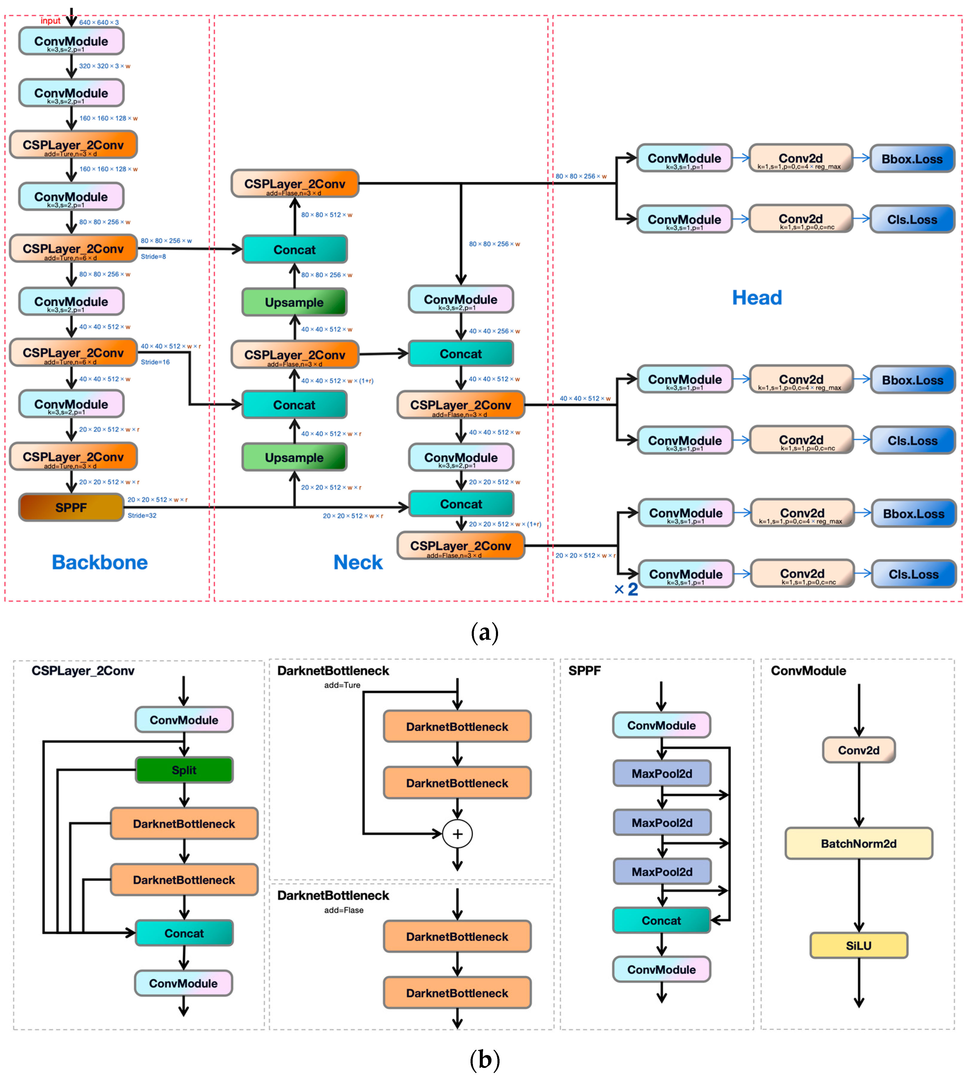
The YOLOv8 algorithm can be divided into five versions: YOLOv8n, YOLOv8s, YOLOv8m, YOLOv8l, and YOLOv8x. According to the network structure diagram, YOLOv8 consists of four parts: Input, Backbone, Neck, and Head. The specific structure is shown in Figure 2. The input end is responsible for scaling the input image to the size required for training. It includes data augmentation operations such as scaling, adjusting the image color tone, and data augmentation to enhance the robustness and generalization of the network model. The backbone network is mainly composed of Conv, C2f, and SPPF modules for feature extraction. The neck section is utilized to improve the fusion of features from different dimensions, specifically the FPN + PAN structure. The head section will calculate and predict the enhanced features, and ultimately determine the confidence level for each label in the output.

2.3. Improved YOLOv8n Model

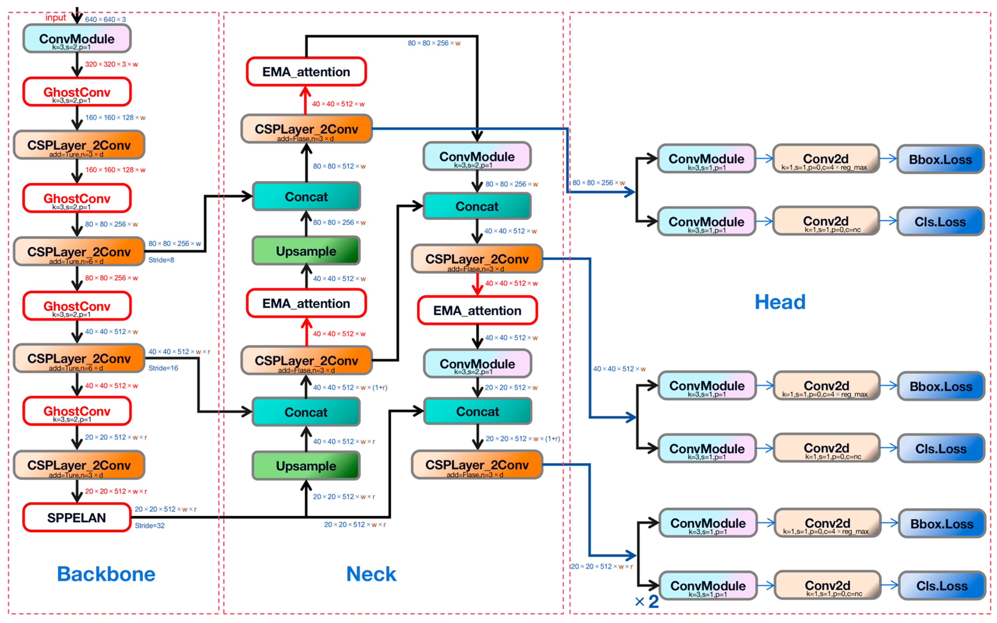
During the growth process of pitaya, it is susceptible to the influence of light and environmental factors. Fruits grown on the same stem may have different sizes and colors. To address this phenomenon, we have created a dataset containing multiple maturity levels with unclear differences in adjacent fruit characteristics, enhancing the robustness of the model. In addition, there is also a problem of mutual occlusion between adjacent fruits, making it difficult to accurately identify the maturity of the fruits. Although existing convolutional neural network models based on deep learning have high detection accuracy, they have drawbacks such as large model calculation parameters, complex calculations, slow detection speed, and significant model memory occupation. Therefore, this article proposes a lightweight pitaya maturity recognition model based on an improved YOLOv8n to address the aforementioned issues, as illustrated in Figure 3.
Firstly, we replaced the ordinary convolutional layer in the backbone network with GhostConv to minimize computational parameters while ensuring accuracy [24]. Next, we substituted SPPELAN for SPPF in the ninth layer [25]. We also incorporated the attention mechanism, EMA_attention, in the Neck. Finally, we adapted the original CIoU to WIoU to address the issue of BBR balance between better and worse quality samples [26,27].

2.3.1. GhostConv Convolutional Module

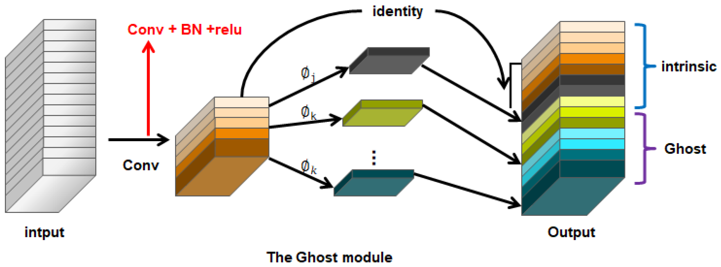
Ghost Net combines linear operations and ordinary convolutions to produce similar feature maps by linearly transforming the feature maps generated by ordinary convolutions [28]. This approach leads to high-dimensional convolution effects, reducing model parameters and computational complexity. The module that combines convolution and linear operations is called the Ghost module. The network structure is shown in Figure 4.
The phantom convolution first aggregates information features between channels through 1 × 1 convolution, and then uses grouped convolution to generate new feature maps. The specific steps are as follows:
(1)
Firstly, we use conventional ordinary convolution to obtain the Y (intrinsic feature maps), which requires approximately the same amount of computation (ignoring bias terms). Here, X is the input and f is the convolution.
Y = X f
(2)
Then, we use i j   to generate the Ghost feature map y i j for each channel of Y′:
y i j = i j y i ,       i = 1 , , m ,       j = 1 , , s ,
(3)
Finally, we concatenate the original feature map obtained in the first step with the Ghost feature map obtained in the second step (identity concatenation) to obtain the final result.
The Ghost Module is divided into two steps to obtain the same number of feature maps as regular convolutions:
  • Step 1: A small number of convolutions are used (e.g., instead of using the typical 128 convolution kernels, only 64 are used here to reduce the computational load by half);
  • Step 2: Cheep operations, represented by ∅ in the graph, such as convolutions with ∅ of 3 × 3 and 5 × 5, and depth-wise convolutions are performed on each feature map.

2.3.2. SPPELAN Pyramid Pooling Structure

SPPELAN is an enhanced module structure based on SPP [29], comprising a CBS module and three Maxpool2d modules for max pooling. The three max-pooling modules are connected sequentially and then fused. This method efficiently extracts the optimal features, passes them sequentially to Concat, and then proceeds through a CBS module to form SPPELAN. The network structure is shown in Figure 5. The SPPELAN module addresses the issue of repetitive feature extraction related to graphs in convolutional networks while maintaining the receptive field unchanged. This significantly enhances the speed of generating candidate boxes, reduces computational costs, and ultimately leads to improved speed.

2.3.3. EMA_Attention Attention Mechanism

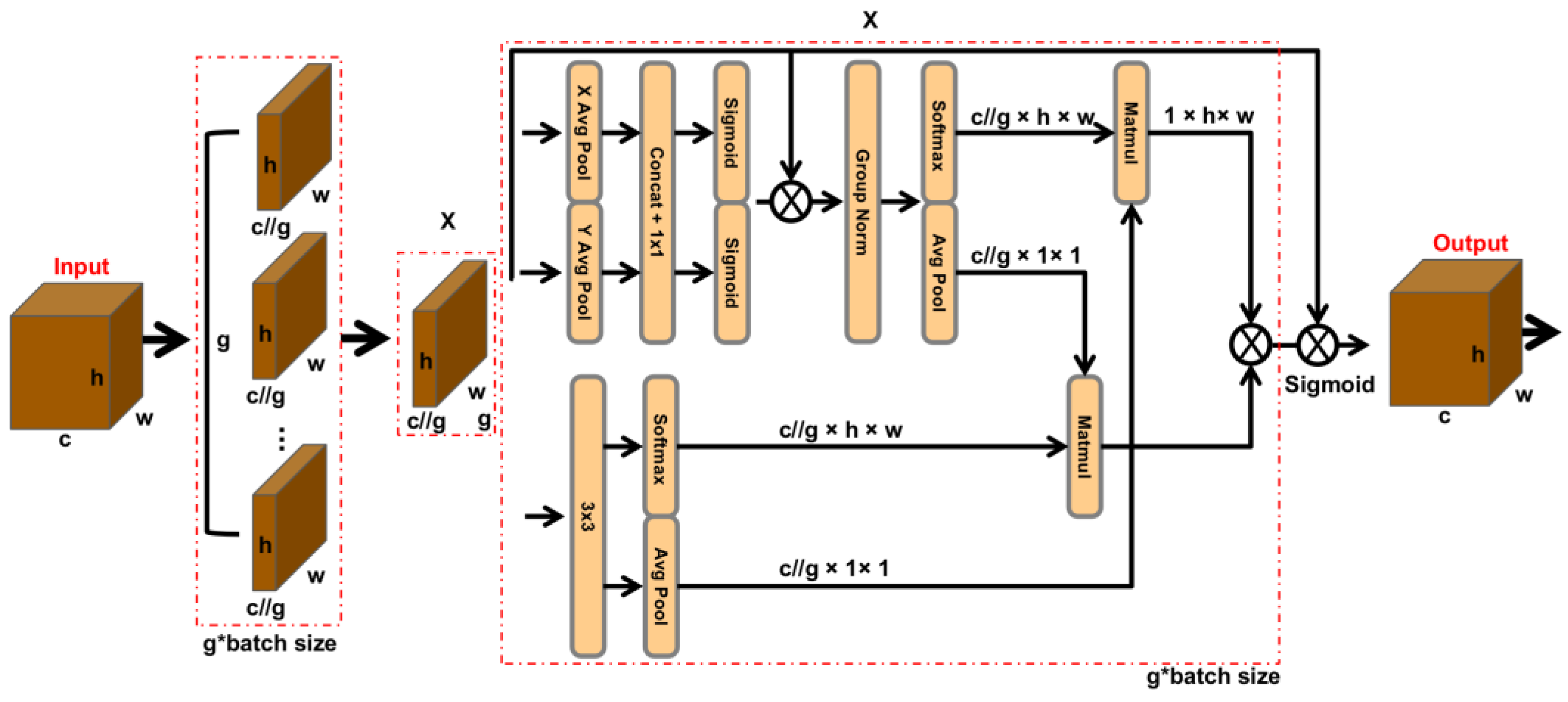
The traditional lightweight approach involves reducing the computational parameters of the model [30]. However, in some cases, parameter reduction may result in feature loss and decreased accuracy. To address this issue, we employ the EMA attention mechanism, an efficient multi-scale attention mechanism that does not necessitate dimensionality reduction [31]. It preserves the information on each channel, reduces computation, reshapes some channels into batch dimensions, and groups channel dimensions into multiple sub-features to evenly distribute spatial semantic features in each feature group. The network structure is shown in Figure 6. Certain channel dimensions are reshaped to batch dimensions to prevent reduction in spatial dimensions through convolution. Local cross-channel interactions are constructed within each parallel subnetwork without reducing channel dimensions, and the output feature maps of the two parallel subnetworks are integrated using cross-spatial learning methods.

2.3.4. WIoU Loss Function

The loss function is used to evaluate the extent to which the predicted value of a model deviates from the true value. The smaller the loss function, the better the performance of the model. Geometric metrics, such as distance and aspect ratio, can magnify the impact of low-quality examples in the dataset, resulting in a reduction in the model’s ability to generalize. The loss function should not overly interfere with training in order to enhance the model’s generalization ability. We have replaced the loss function CIoU of the original YOLOv8n model with WIoU to expedite the convergence of the model and enhance its generalization ability and robustness.
The traditional IoU (Intersection over Union) only considers the overlap between the predicted box and the true box [32], without taking into account the area between the predicted box and the true box, which could introduce bias in the evaluation results. WIoU (Wise IoU) features dynamic non-monotonic FM. The specific definition and formula of WIoU are as follows [33]:
(1)
Wise IoU v1: Distance attention was constructed based on distance metrics, resulting in Wise IoU v1 with a two-layer attention mechanism:
R W I o U 1 , e , which will significantly amplify L I o U in the case of the ordinary-quality anchor box.
L I o U 0 , 1 , which will have a pronounced influence on the R W I o U , particularly in the case of high-quality anchor boxes, whereby the distance between the centre points is given significant weight when the anchor box exhibits a high degree of overlap with the target box.
L W I o U v 1 = R W I o U L I o U
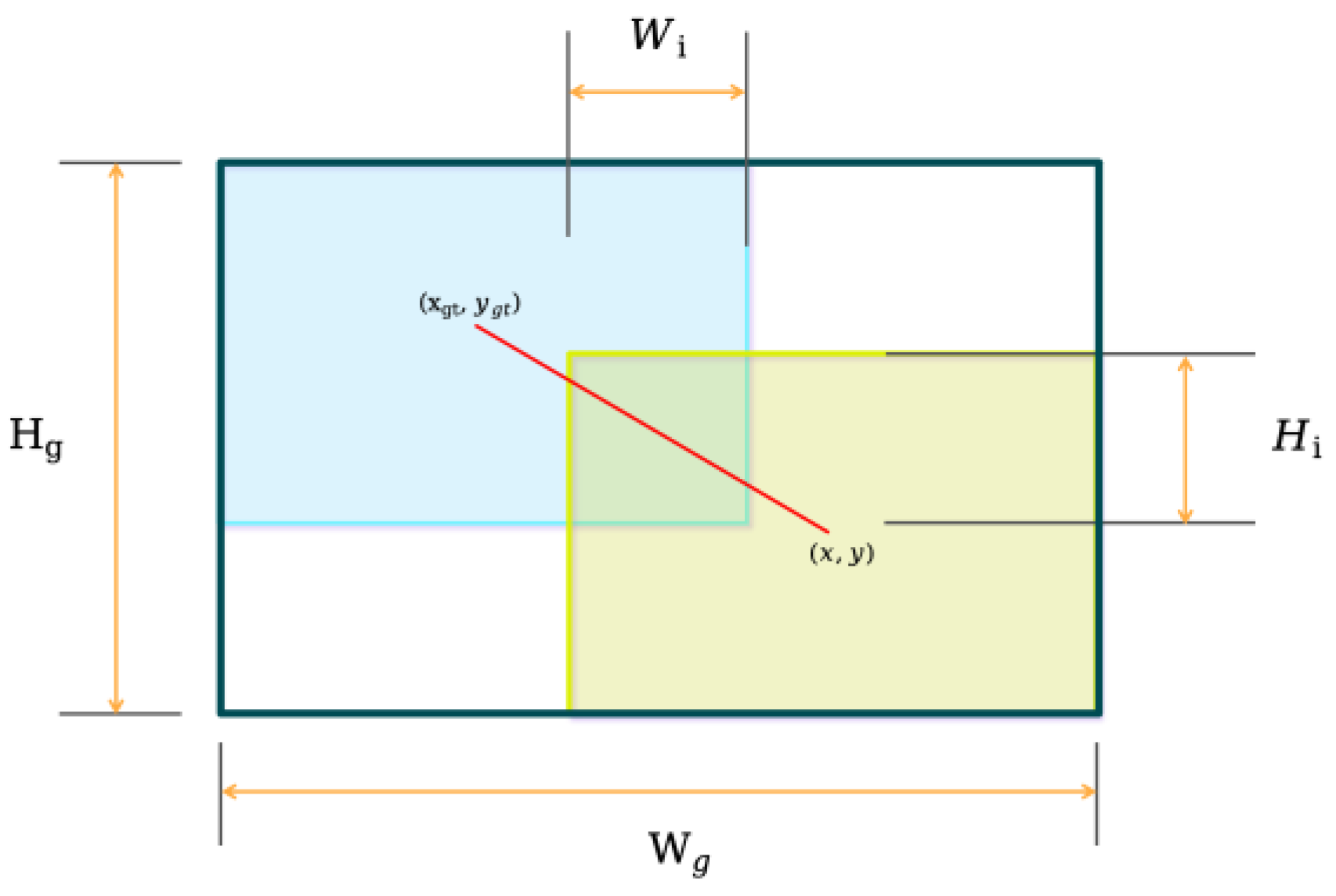
R W I o U = e x p x x g t 2 + y y g t 2 W g 2 + H g 2 *
where W g ,   H g are the size of the smallest enclosing box, as shown in Figure 7. In order to prevent R W I o U from generating gradients that impede convergence, W g and H g are separated from the computational graph (this is indicated by the superscript *). As a consequence of the effective removal of the impediments to convergence, the introduction of new metrics, such as aspect ratios, was not deemed necessary.
Figure 7 illustrates the smallest bounding box (dark green) and the connection of the center point (red), where the area of the union is as follows:
S u = w h + w g t h g t W i W i
(2)
Wise IoU v2: A monotonic focusing mechanism, WIoU v2, for cross-entropy was designed based on Focal Loss. This mechanism effectively reduces the influence of inter-examples on the loss value, the monotone focusing coefficient L I o U γ .
L W I o U v 2 = L I o U γ L W I o U v 1 ,   γ > 0
The gradient of the WIoU v2 backpropagation is subject to alteration as a consequence of the introduction of the focusing coefficient.
L W I o U v 2 L I o U = L I o U γ L W I o U v 1 L I o U ,   γ > 0
It should be noted that the gradient gain is L I o U γ 0 , 1 . During the training of the model, the gradient gain decreases as L I o U decreases, which results in slower convergence in the later stages of training. Therefore, the average value of L I o U is introduced as a normalizing factor.
  L W I o U v 2 = L I o U L I o U ¯ γ L W I o U v 1
In this context, L I o U ¯ represents the running mean with momentum m. By dynamically updating the normalising factor, the gradient gain L I o U L I o U ¯ γ is maintained at a high level, thereby addressing the issue of slow convergence observed in the late stages of training.
In the dynamic non-monotonic FM, the discrete length of the anchor box is expressed as the ratio of L I o U to L I o U ¯ .
β = L I o U L I o U ¯ 0 ,                              
(3)
Wise-IoU v3: A Wise-IoU v3 with dynamic non-monotonic FM is obtained by constructing a non-monotonic focusing coefficient using β and applying it to Wise-IoU v1.
The presence of a small outlier is indicative of the high quality of the anchor frame. Furthermore, the assignment of a smaller gradient gain to anchors with larger outliers will effectively prevent the emergence of large harmful gradients from low-quality examples. A non-monotonic focusing coefficient was constructed using β and subsequently applied to the WIoU v1. The variables δ and α represent hyperparameters. The variable r represents the gradient gain, which is controlled by δ and α. It should be noted that δ is equal to r = 1 when β = δ.
L W I o U v 3 = r L W I o U v 1 ,   r = β δ α β δ                

2.4. Experimental Environment Configuration and Network Parameter Settings

The operating system used for the test was Windows 11 Professional. The CPU model was 13th Gen Intel(R) Core(TM) i9-13900K 3.00 GHz, Guangdong, China, Intel Corporation, the GPU model was NVIDIA GeForce RTX 4090, the RAM was 64 GB, with 4 TB SSD*2,Guangdong, China, Intel Corporation and the programming language used was Python 3.8. The deep learning framework used is PyTorch (torch-2.1.1+cu118).

2.5. Model Evaluation Indicators

We typically need to assess quantitative evaluation indicators to determine the effectiveness of the object detection algorithm’s detection results. In order to ensure the objectivity and effectiveness of the experiment, we will use the following indicators to evaluate the model: accuracy (Precision), recall (Recall), F1 score value, mean accuracy (mAP—Mean Average Precision), and model size.
The corresponding evaluation indicators defined above are as follows:
P ( P r e c i s i o n ) = T P F P + T P
R ( R e c a l l ) = T P F N + T P
F 1   s c o r e = 2 × P r e s i c i o n × R e c a l l P r e c i s i o n + R e c a l l = 2 T P 2 T P + F P + F N
A P = k = 0 k = n 1 [ R e c a l l s ( k ) R e c a l l s ( k + 1 ) ] P r e c i s i o n ( k ) d
R e c a l l s ( n ) = 0 , P r e c i s i o n s ( n ) = 1
n = t h e   n u m b e r   o f   c l a s s e s
m A P = 1 n k = 1 k = n A P k
A P k = t h e   A P   o f   c l a s s   k
n = t h e   n u m b e r   o f   c l a s s s e s
TP (True Positive) is the number of examples that the model predicts to be positive but the actual label is also positive. FP (False Positive) stands for false positive-that is, the number of instances where the model predicted the positive class but the actual label was negative. FN (False Negative) is the number of false negatives that the model predicted to be negative but were actually labeled positive.TN (True Negative) stands for the number of true negative examples, that is, the number of instances where the model predicts the negative class and the actual label is also negative.
In general, Precision (P) represents the detection accuracy of the target detector at an Intersection over Union (IoU) of 0.5. Precision is the percentage of positive samples in the predicted results. On the other hand, Recall rate (R) is the detection recall rate of the target detector at an IoU of 0.5. Recall rate is the percentage of predicted positive samples in the actual positive samples. However, both accuracy and recall have their limitations: when the threshold is set high, accuracy increases, but a significant amount of data may be overlooked. If the threshold is set low, the recall rate will be high, but the predicted results will be very inaccurate. It can be concluded that accuracy and recall are mutually exclusive. To balance these two indicators, we introduce the F1 score value for comprehensive evaluation. We utilize Mean Average Precision (mAP), where AP (Average Precision) represents the area under the Precision-Recall (PR) curve within the range of 0–1. Compared to a single metric, Average Precision (AP) can reflect the overall precision at various recall rates. Adding all average precisions (APs) and calculating the average yields mAP, which better represents the detection performance of the detector.

3. Experimental Results and Analysis

3.1. Improved YOLOv8n Test

In order to verify the performance of the improved YOLOv8n model, we tested and evaluated 278 pitaya fruit images in the test set. The results of this testing are presented in Table 1. By analyzing Table 1, it is evident that the algorithm achieves an average accuracy of 90.9%, with an accuracy rate of 85.2% and a recall rate of 87.3%. All maturity detection results are close to 90%.
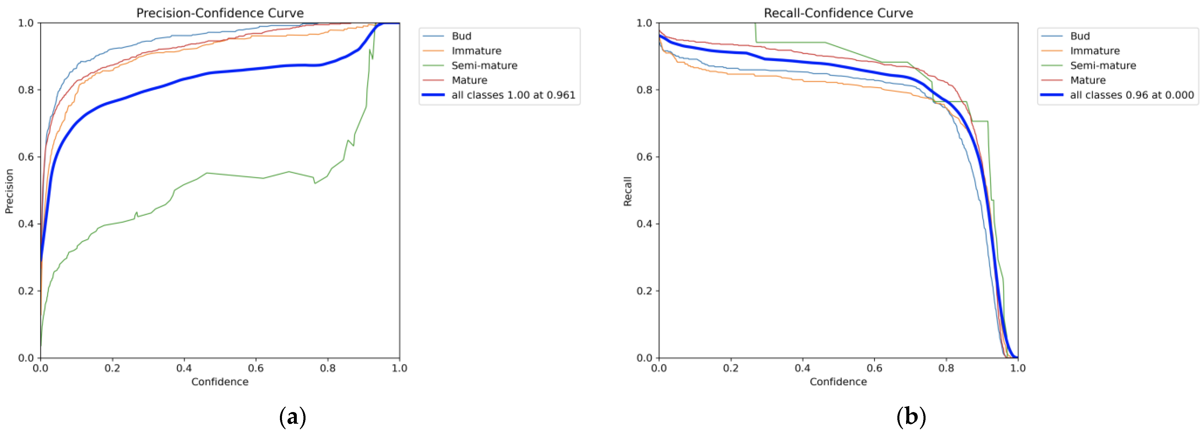
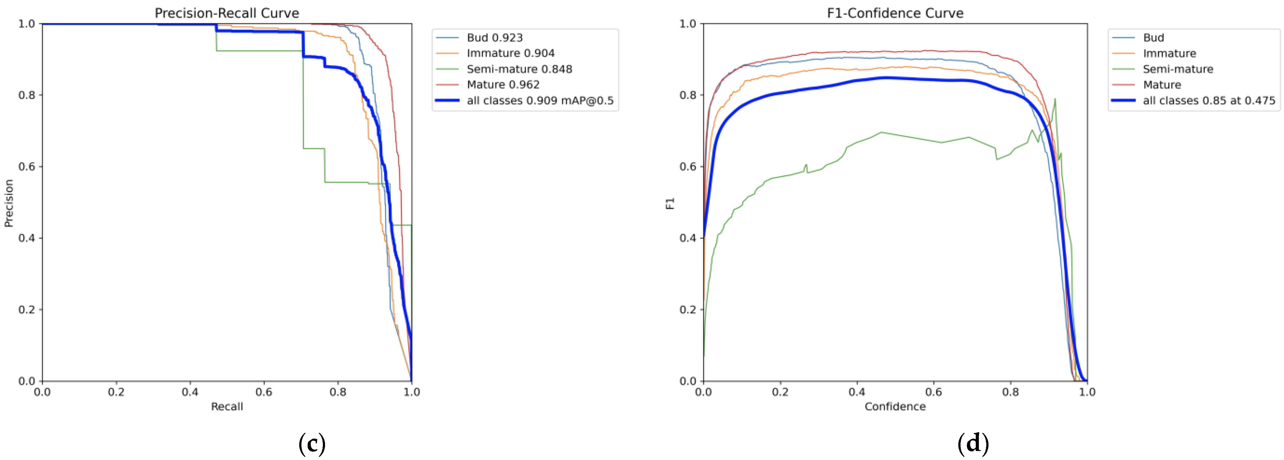
In order to more accurately reflect the detection data, various indicator curves of the improved model have been drawn, as shown in Figure 8.
In Figure 8a, the horizontal axis represents the confidence and the vertical axis represents the accuracy. The shape and position of the curve can be used to evaluate the performance and stability of the model, and the curve has a positive slope. The graph illustrates the accuracy of the model at different confidence levels. With an increase in confidence, the accuracy will correspondingly improve, this situation represents an enhanced detection performance of the model, or in other words, a higher degree of accuracy in identifying the maturity of pitaya fruit.
Figure 8b depicts the relationship between confidence and recall, with the horizontal axis representing confidence and the vertical axis representing recall. Each data point in the graph represents the recall rate under a specific confidence level. In the graph, the closer the curve is to the upper right corner, the more effective the model’s performance. When the curve is situated in close proximity to the upper right corner, it signifies that the model is capable of maintaining a high recall rate while concurrently exhibiting a high degree of confidence.
Figure 8c depicts the relationship between the recall rate and the accuracy rate, with the horizontal axis representing the former and the vertical axis representing the latter. In general, a high recall rate is associated with a low accuracy rate, while a high accuracy rate is associated with a low recall rate. The precision-recall curve represents a relatively balanced evaluation index between accuracy and recall. As the curve approaches the upper right corner, it indicates that the model can maintain high accuracy and recall in prediction, thereby indicating that the prediction results are more accurate.
Figure 8d depicts the relationship between confidence and F1 score, with the horizontal axis representing confidence and the vertical axis representing F1 score. The F1 Confidence Curve is a curve on which the F1 score gradually changes with increasing confidence. The model does not categorically determine the class to which an object belongs; rather, it assigns a probability to the object in question. The threshold, or confidence, is the set threshold. If the probability of the object recognized by the model exceeds the threshold, it is considered to belong to this class. If the value is below the threshold, it is deemed to not belong to this class.
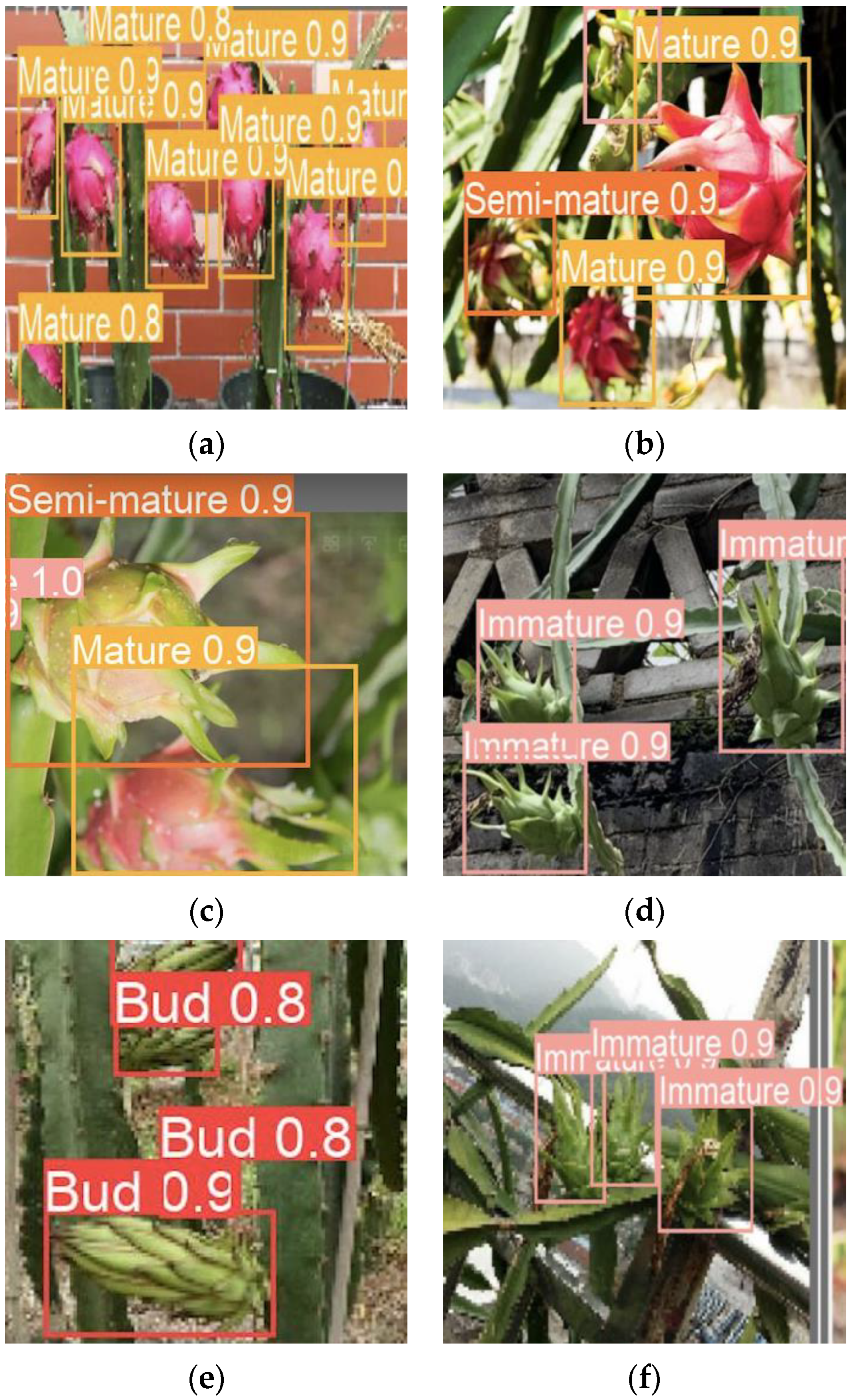
Part of the detection images are shown in Figure 9. From Figure 9a, it can be seen that our improved YOLOv8n model can accurately identify and prevent missed detections when multiple targets are present. From Figure 9b,c, it can be seen that the improved algorithm can accurately identify the fruit ripeness of pitayas at various maturity levels without any misjudgment. From Figure 9d, Figure 9e,f, it can be seen that our improved YOLOv8n model can accurately recognize pitaya ripeness even in the presence of objects with similar pitaya color interference, stems obstructing fruits and blurred images. During the growth cycle of pitaya, the shape and color of the fruit undergo significant changes due to the influence of light and the natural environment, leading to varying levels of fruit ripeness. Some adjacent fruits have small differences, and the color change of pitaya is not obvious, especially in the late and early stages of ripening, which can be confusing. The improved algorithm can efficiently extract the optimal color features to accurately recognize pitayas at various maturity levels.
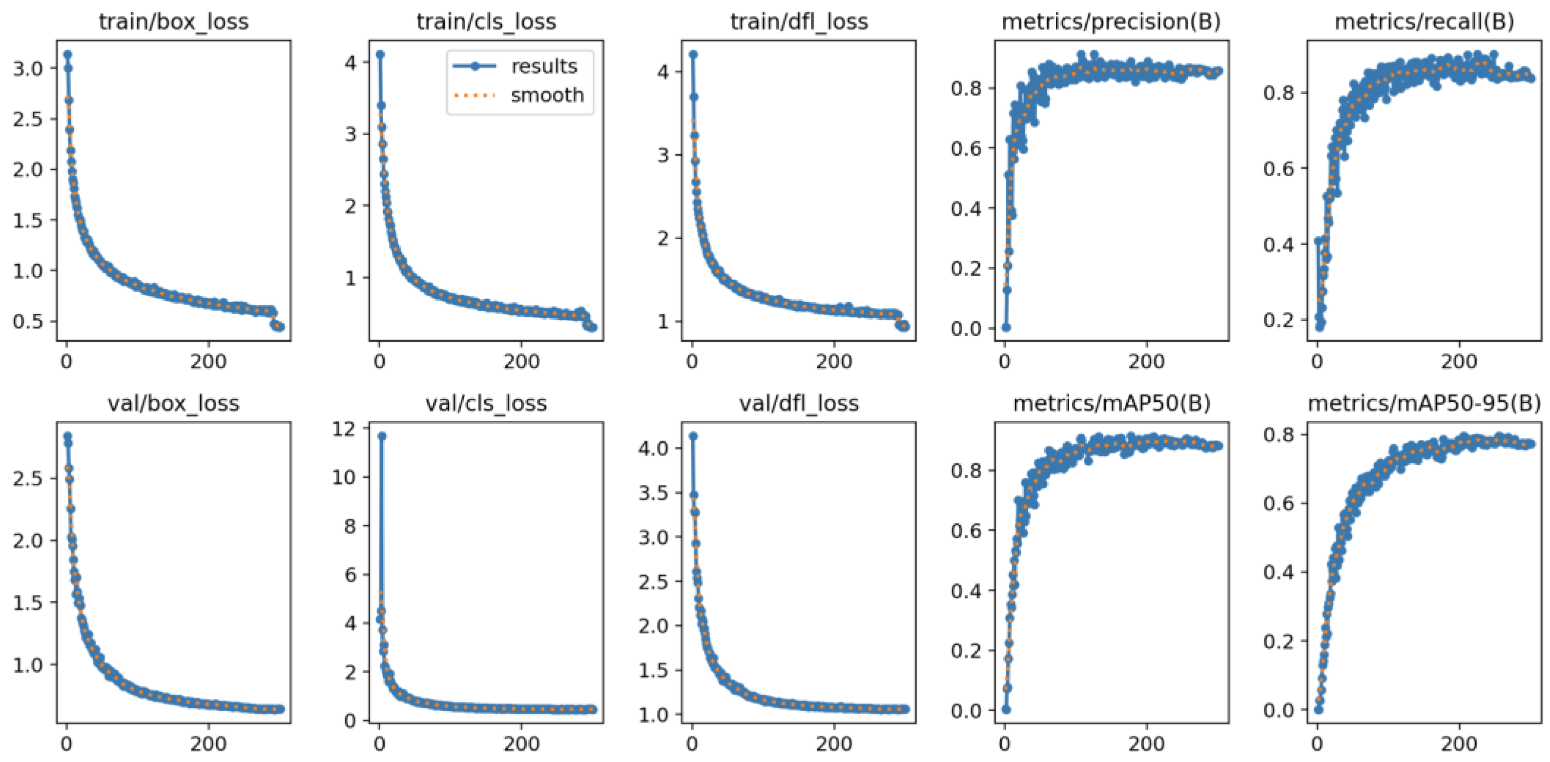
In order to provide further insight into the model’s performance, we have plotted the visualized training result curves and detection heatmaps of the improved model, as shown in Figure 10 and Figure 11. As can be seen from Figure 10, the model gradually begins to converge and stabilize after 100–120 epochs of loss, and there is no incremental increase in the loss curve at the end. With regard to the precision, recall, mAP50 and mAP50-95 curves, it can be observed that they begin to converge after 90 epochs, with a more pronounced effect.
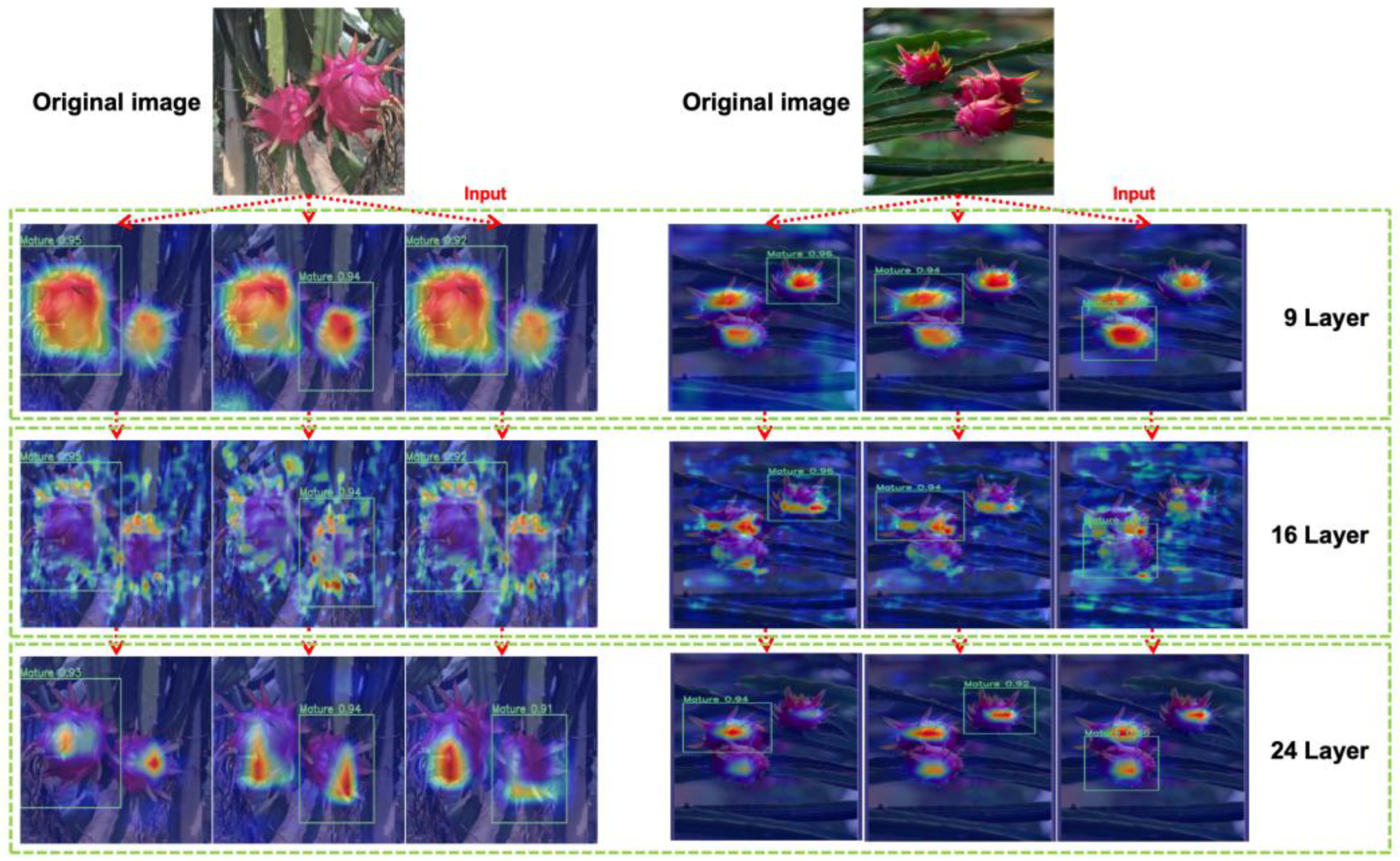
A heatmap is a visualization technique employed for the purpose of object detection. The distribution of the heatmap allows the intensity distribution of the model in the input image to be displayed, thus enabling the identification of important areas within the image. The brightness or darkness of the color indicates the degree of importance attributed to the detection area of the model, thereby indicating the level of confidence the model has in the area being identified as pitaya fruit. The darker or lighter the color, the lower the confidence of the pitaya fruit in the area. As illustrated in Figure 11, the heat maps of the 9th, 16th, and 24th layers were generated. The enhanced model is capable of concentrating on the precise location of the pitaya fruit during detection, thereby facilitating the accurate delineation of the range of the pitaya fruit for prediction.
In summary, our improved YOLOv8n model demonstrates high accuracy. When there are too many targets or occlusions, our improved model can accurately identify the ripeness of pitaya, significantly reducing missed and false detections. Our improved model can accurately detect the ripeness of pitaya in various natural environments. It exhibits strong robustness and generalizable capabilities.

3.2. Improvement of YOLOv8n Ablation Test

In order to further validate the improved YOLOv8n model, we conducted ablation experiments under quantitative conditions. The specific method involves replacing Conv with GhostConv, replacing SPPF with SPPELAN, adding an EMA-attention mechanism, and modifying the loss function to WIoU based on the YOLOv8n model. This experiment also included the original YOLOv8 model as a control and was conducted under quantitative conditions. The evaluation comparison results are shown in Table 2.
It can be seen from Table 2 that our improved YOLOv8n model exhibits higher average accuracy compared to other groups, and it can be observed that the mAP50 value of our improved model steadily rises. The presence of a check mark signifies the incorporation of a module into the test, whereas an unchecked mark denotes the absence of such an addition or replacement.

3.3. Analysis of Comparison Results of Different Object Detection Networks

In order to better compare the performance of our improved YOLOv8n model, we divided the 2788 pitaya images in Section 2.1 into training, validation, and testing sets in a 7:2:1 ratio for model comparison experiments. The compared models include YOLOv5n, YOLOv6n, YOLOv7, YOLOv8n (baseline), and the improved YOLOv8n model. We performed 300 epochs of iterations in the same scenario to ensure the objectivity and fairness of the experiment. The results of the model comparison are presented in Table 3.
As shown in Table 3, our improved YOLOv8n model achieves an accuracy (P) of 85.2%, a recall rate of 87.3%, an F1-Score of 86.23, 2,660,358 calculation parameters, a mAP50 of 90.9%, and a compact model size of only 5.30MB. As can be seen from Table 3, our improved model demonstrates good performance across all indicators, particularly excelling in the average accuracy mAP50, surpassing other models.
Compared with YOLOv6n, the accuracy rate of our improved YOLOv8n model decreased by 1.8%, the F1 score decreased by 0.56, but the recall rate increased by 0.7%. Additionally, the computational parameters decreased by 46.85%, the model size reduced by 4.68MB, and the mAP50 increased by 3.2%. Compared to YOLOv5n and YOLOv7, the accuracy of our improved YOLOv8n model increased by 2.7% and 0.5%, respectively. The recall rate decreased by 2.7% compared to YOLOv5n and increased by 0.1% compared to YOLOv7. Additionally, the F1 score decreased by 2.67 compared to YOLOv5n. Compared with YOLOv7, it increased by 0.3, increased by 33.67% compared with YOLOv5n in terms of parameters, and decreased by 92.85% compared with YOLOv7. On mAP50, our improved YOLOv8n model is 3.2% and 2.6% higher than YOLOv6n and YOLOv7, respectively. The model size is 1.66MB larger than YOLOv5n and 66MB smaller than YOLOv7. For the original YOLOv8n model, the accuracy rate of our improved YOLOv8n model decreased by 0.9%. However, the recall rate and F1 score increased by 1.8% and 6.35, respectively. The calculation parameter decreased by 11.51%, the mAP50 increased by 1.2%, and the model size decreased by 0.64MB. In summary, our improved YOLOv8n model can fulfill the demands for precise detection in real-world natural settings, guaranteeing both high detection accuracy and an optimal model size.

4. Conclusions

In order to achieve rapid recognition of pitaya targets in natural environments, we focus on pitaya maturity as the research object. During the growth process, pitaya undergoes changes in its shape and color, with each stage exhibiting significant characteristics. Therefore, we divided the pitaya into four stages according to different maturity levels, namely Bud, Immature, Semi-mature and Mature, and we have designed a lightweight detection and classification network for recognizing the maturity of pitaya fruit based on the YOLOv8n algorithm, namely GSE-YOLO (GhostConv SPPELAN-EMA-YOLO), which addresses the issue of low efficiency in the traditional assessment of pitaya ripeness. In order to enhance model performance, we modified the backbone structure of the YOLOv8n model. To reduce computational complexity, we employed GhostConv instead of regular convolution and incorporated an attention mechanism to prevent feature loss. Modifying the loss function led to improved convergence of the model.
The results show that the improved YOLOv8n model proposed in this paper has achieved a good recognition effect, with mAP50 reaching 90.9% and a model size of only 5.3MB. This model can accurately detect objects in a natural environment, ensuring higher accuracy while maintaining a lighter YOLOv8n model, aligning with the current trend of lightweight intelligent models.

Author Contributions

Z.H. and Z.Q. are co-first authors. Conceptualization, Z.Q. and X.T. (Xinyuan Tian); methodology, Z.H.; software, Z.Q.; validation, D.M. and X.T. (Xuejun Tian); formal analysis, Z.H.; investigation, D.M.; resources, X.T. (Xuejun Tian); data curation, Z.H.; writing—original draft preparation, Z.Q.; writing—review and editing, Z.H.; visualization, D.M.; supervision, Z.H.; project administration, Z.Q.; funding acquisition, X.T. (Xinyuan Tian). All authors have read and agreed to the published version of the manuscript.

Funding

This research was funded by Research on Intelligent Monitoring Technology of Pitaya Growth Cycle Based on Machine Vision (Grant No. 2023ZDZX4031), the Special Talent Fund of Lingnan Normal University (ZL22026).

Data Availability Statement

The original contributions presented in the study are included in the article, further inquiries can be directed to the corresponding author.

Conflicts of Interest

The authors declare no conflicts of interest.

References

  1. Nan, Y.; Zhang, H.; Zeng, Y.; Zheng, J.; Ge, Y. Intelligent detection of Multi-Class pitaya fruits in target picking row based on WGB-YOLO network. Comput. Electron. Agric. 2023, 208, 107780. [Google Scholar] [CrossRef]
  2. Fang, W.; Wu, Z.; Li, W.; Sun, X.; Mao, W.; Li, R.; Majeed, Y.; Fu, L. Fruit detachment force of multiple varieties kiwifruit with different fruit-stem angles for designing universal robotic picking end-effector. Comput. Electron. Agric. 2023, 213, 108225. [Google Scholar] [CrossRef]
  3. Wang, C.; Sun, W.; Wu, H.; Zhao, C.; Teng, G.; Yang, Y.; Du, P. A Low-Altitude Remote Sensing Inspection Method on Rural Living Environments Based on a Modified YOLOv5s-ViT. Remote Sens. 2022, 14, 4784. [Google Scholar] [CrossRef]
  4. Ma, H.; Liu, Y.; Ren, Y.; Yu, J. Detection of Collapsed Buildings in Post-Earthquake Remote Sensing Images Based on the Improved YOLOv3. Remote Sens. 2019, 12, 44. [Google Scholar] [CrossRef]
  5. Su, X.; Zhang, J.; Ma, Z.; Dong, Y.; Zi, J.; Xu, N.; Zhang, H.; Xu, F.; Chen, F. Identification of Rare Wildlife in the Field Environment Based on the Improved YOLOv5 Model. Remote Sens. 2024, 16, 1535. [Google Scholar] [CrossRef]
  6. Ding, W.; Abdel-Basset, M.; Alrashdi, I.; Hawash, H. Next generation of computer vision for plant disease monitoring in precision agriculture: A contemporary survey, taxonomy, experiments, and future direction. Inf. Sci. 2024, 665, 120338. [Google Scholar] [CrossRef]
  7. Lu, Y.; Young, S. A survey of public datasets for computer vision tasks in precision agriculture. Comput. Electron. Agric. 2020, 178, 105760. [Google Scholar] [CrossRef]
  8. Patrício, D.I.; Rieder, R. Computer vision and artificial intelligence in precision agriculture for grain crops: A systematic review. Comput. Electron. Agric. 2018, 153, 69–81. [Google Scholar] [CrossRef]
  9. Tian, Y.; Wang, S.; Li, E.; Yang, G.; Liang, Z.; Tan, M. MD-YOLO: Multi-scale Dense YOLO for small target pest detection. Comput. Electron. Agric. 2023, 213, 108233. [Google Scholar] [CrossRef]
  10. Xu, J.; Lu, Y.; Olaniyi, E.; Harvey, L. Online volume measurement of sweetpotatoes by A LiDAR-based machine vision system. J. Food Eng. 2024, 361, 111725. [Google Scholar] [CrossRef]
  11. Wang, K.; Li, Z.; Li, J.; Lin, H. Raman spectroscopic techniques for nondestructive analysis of agri-foods: A state-of-the-art review. Trends Food Sci. Technol. 2021, 118, 490–504. [Google Scholar] [CrossRef]
  12. Wang, D.; He, D. Channel pruned YOLO V5s-based deep learning approach for rapid and accurate apple fruitlet detection before fruit thinning. Biosyst. Eng. 2021, 210, 271–281. [Google Scholar] [CrossRef]
  13. Jiang, Y.; Bian, B.; Zheng, B.; Chu, J. A time space network optimization model for integrated fresh fruit harvest and distribution considering maturity. Comput. Ind. Eng. 2024, 190, 110029. [Google Scholar] [CrossRef]
  14. Mazen, F.M.A.; Nashat, A.A. Ripeness Classification of Bananas Using an Artificial Neural Network. Arab. J. Sci. Eng. 2019, 44, 6901–6910. [Google Scholar] [CrossRef]
  15. Fu, L.; Wu, F.; Zou, X.; Jiang, Y.; Lin, J.; Yang, Z.; Duan, J. Fast detection of banana bunches and stalks in the natural environment based on deep learning. Comput. Electron. Agric. 2022, 194, 106800. [Google Scholar] [CrossRef]
  16. Mim, F.S.; Galib, S.M.; Hasan, M.F.; Jerin, S.A. Automatic detection of mango ripening stages—An application of information technology to botany. Sci. Hortic. 2018, 237, 156–163. [Google Scholar] [CrossRef]
  17. Kalopesa, E.; Gkrimpizis, T.; Samarinas, N.; Tsakiridis, N.L.; Zalidis, G.C. Rapid Determination of Wine Grape Maturity Level from pH, Titratable Acidity, and Sugar Content Using Non-Destructive In Situ Infrared Spectroscopy and Multi-Head Attention Convolutional Neural Networks. Sensors 2023, 23, 9536. [Google Scholar] [CrossRef] [PubMed]
  18. Silva, R.; Freitas, O.; Melo-Pinto, P. Evaluating the generalization ability of deep learning models: An application on sugar content estimation from hyperspectral images of wine grape berries. Expert Syst. Appl. 2024, 250, 123891. [Google Scholar] [CrossRef]
  19. Mohammadi, V.; Kheiralipour, K.; Ghasemi-Varnamkhasti, M. Detecting maturity of persimmon fruit based on image processing technique. Sci. Hortic. 2015, 184, 123–128. [Google Scholar] [CrossRef]
  20. Attri, I.; Awasthi, L.K.; Sharma, T.P.; Rathee, P. A review of deep learning techniques used in agriculture. Ecol. Inform. 2023, 77, 102217. [Google Scholar] [CrossRef]
  21. Ariza-Sentís, M.; Vélez, S.; Martínez-Peña, R.; Baja, H.; Valente, J. Object detection and tracking in Precision Farming: A systematic review. Comput. Electron. Agric. 2024, 219, 108757. [Google Scholar] [CrossRef]
  22. Gonzales Martinez, R.; van Dongen, D. Deep learning algorithms for the early detection of breast cancer: A comparative study with traditional machine learning. Inform. Med. Unlocked 2023, 41, 101317. [Google Scholar] [CrossRef]
  23. Ma, B.; Hua, Z.; Wen, Y.; Deng, H.; Zhao, Y.; Pu, L.; Song, H. Using an improved lightweight YOLOv8 model for real-time detection of multi-stage apple fruit in complex orchard environments. Artif. Intell. Agric. 2024, 11, 70–82. [Google Scholar] [CrossRef]
  24. Liu, G.; Hu, Y.; Chen, Z.; Guo, J.; Ni, P. Lightweight object detection algorithm for robots with improved YOLOv5. Eng. Appl. Artif. Intel. 2023, 123, 106217. [Google Scholar] [CrossRef]
  25. Ma, W.; Guan, Z.; Wang, X.; Yang, C.; Cao, J. YOLO-FL: A target detection algorithm for reflective clothing wearing inspection. Displays 2023, 80, 102561. [Google Scholar] [CrossRef]
  26. Gao, S.; Chu, M.; Zhang, L. A detection network for small defects of steel surface based on YOLOv7. Digit. Signal Process. 2024, 149, 104484. [Google Scholar] [CrossRef]
  27. Wang, A.; Qian, W.; Li, A.; Xu, Y.; Hu, J.; Xie, Y.; Zhang, L. NVW-YOLOv8s: An improved YOLOv8s network for real-time detection and segmentation of tomato fruits at different ripeness stages. Comput. Electron. Agric. 2024, 219, 108833. [Google Scholar] [CrossRef]
  28. Kothala, L.P.; Jonnala, P.; Guntur, S.R. Localization of mixed intracranial hemorrhages by using a ghost convolution-based YOLO network. Biomed. Signal Process. Control 2023, 80, 104378. [Google Scholar] [CrossRef]
  29. Huang, Z.; Wang, J.; Fu, X.; Yu, T.; Guo, Y.; Wang, R. DC-SPP-YOLO: Dense connection and spatial pyramid pooling based YOLO for object detection. Inf. Sci. 2020, 522, 241–258. [Google Scholar] [CrossRef]
  30. Zhang, P.; Dai, N.; Liu, X.; Yuan, J.; Xin, Z. A novel lightweight model HGCA-YOLO: Application to recognition of invisible spears for white asparagus robotic harvesting. Comput. Electron. Agric. 2024, 220, 108852. [Google Scholar] [CrossRef]
  31. Xie, T.; Wang, Z.; Li, H.; Wu, P.; Huang, H.; Zhang, H.; Alsaadi, F.E.; Zeng, N. Progressive attention integration-based multi-scale efficient network for medical imaging analysis with application to COVID-19 diagnosis. Comput. Biol. Med. 2023, 159, 106947. [Google Scholar] [CrossRef] [PubMed]
  32. Cai, H.; Lan, L.; Zhang, J.; Zhang, X.; Zhan, Y.; Luo, Z. IoUformer: Pseudo-IoU prediction with transformer for visual tracking. Neural Netw. 2024, 170, 548–563. [Google Scholar] [CrossRef] [PubMed]
  33. Du, X.; Cheng, H.; Ma, Z.; Lu, W.; Wang, M.; Meng, Z.; Jiang, C.; Hong, F. DSW-YOLO: A detection method for ground-planted strawberry fruits under different occlusion levels. Comput. Electron. Agric. 2023, 214, 108304. [Google Scholar] [CrossRef]
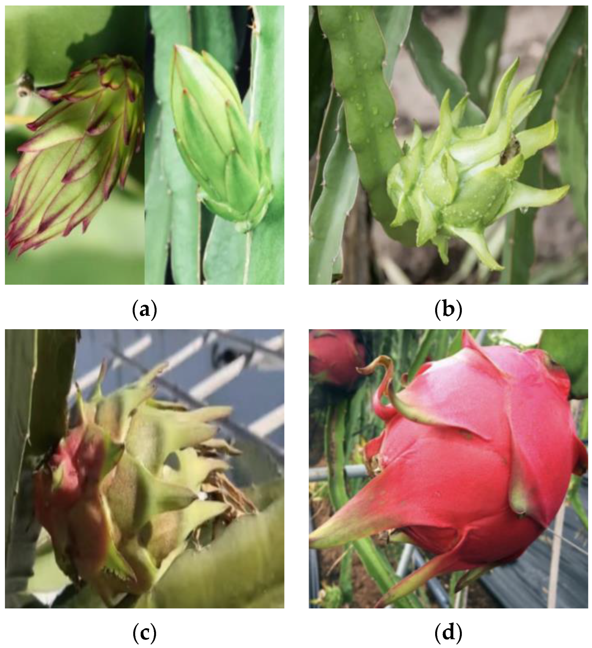
Figure 1. Classification of ripeness of pitaya fruits. (a) Bud. (b) Immature. (c) Semi-mature. (d) Mature.
Horticulturae 10 00852 g001
Figure 2. YOLOv8 neural network structure diagram. (a) YOLOv8 network structure diagram. (b) Specific module diagram.
Horticulturae 10 00852 g002
Figure 3. Improved network structure diagram.
Horticulturae 10 00852 g003
Figure 4. The Ghost module structure diagram.
Horticulturae 10 00852 g004
Figure 5. SPPELAN module structure diagram.
Horticulturae 10 00852 g005
Figure 6. EMA_attention Module diagram of attention mechanism.
Horticulturae 10 00852 g006
Figure 7. Schematic diagram of the smallest enclosing box.
Horticulturae 10 00852 g007
Figure 8. Curve of various indicators of the improved model. (a) Precision-Confidence Curve. (b) Recall-Confidence Curve. (c) Precision-Recall Curve. (d) F1-Confidence Curve.
Horticulturae 10 00852 g008aHorticulturae 10 00852 g008b
Figure 9. Partial images of pitaya detection. Note: The dataset we used (including the test set) is sourced from open-source images on the internet and field photographs taken by the team.
Horticulturae 10 00852 g009
Figure 10. Visualization training result curve.
Horticulturae 10 00852 g010
Figure 11. Heat map of improved model detection.
Horticulturae 10 00852 g011
Table 1. Testing Results at Different Maturity Levels.
ClassPrecisionRecallF1-ScoremAP50
Bud0.9710.84290.1992.3%
Immature0.9420.82287.7990.4%
Semi-mature0.5490.93169.0784.8%
Mature0.9460.89792.0896.2%
All0.8520.87386.2390.9%
Table 2. Improved YOLOv8n model ablation test results.
GhostConvSPPELANEMA_AttentionWIoUmAP50
YOLOv8n 88.3%
YOLOv8n 89.7%
YOLOv8n 89.8%
YOLOv8n 90.3%
YOLOv8n 90.8%
YOLOv8n90.9%
Table 3. Comparison Table of Test Results of Various Models.
PrecisionRecallF1-ScoreParametersmAP50Weight
YOLOv5n82.5%90.0%88.901,764,57789.4%3.64 MB
YOLOv6n87.0%86.6%86.795,005,90487.7%9.98 MB
YOLOv784.7%87.2%85.9337,212,73888.3%71.3 MB
YOLOv8n86.1%85.5%79.883,006,42889.7%5.94 MB
Ours85.2%87.3%86.232,660,35890.9%5.30 MB
Disclaimer/Publisher’s Note: The statements, opinions and data contained in all publications are solely those of the individual author(s) and contributor(s) and not of MDPI and/or the editor(s). MDPI and/or the editor(s) disclaim responsibility for any injury to people or property resulting from any ideas, methods, instructions or products referred to in the content.