1. Introduction
Since the developing heart and embryo continue to function for some time in the absence of erythrocytes, it appears that the function of the early embryonic heart is not for the purpose of nutrient transport [
1,
2]. Instead, recent work suggests that the heart’s function is to aid in its own growth [
1,
3,
4,
5]. Two important roles for intracardial fluid dynamics in terms of proper cardiogenesis are to exert hemodynamic forces onto the ventricular lining and to advect morphogens [
2,
6]. These two fluid effects help regulate and drive organogenesis in developing embryos. Both shear stress and pressure may be key components to activating developmental regulatory networks by acting on cardiac cells [
7] through a process called mechanotransduction. In this case, mechanical stimuli are transmitted by intracellular signalling pathways to the interior of the cell. Moreover, increased receptor–ligand bond formation may appear near the endothelial lining in regions of higher vorticity [
8], which gives rise to greater mixing of chemical morphogens. These chemicals may act as epigenetic signals, which are then advected throughout the chamber [
9,
10]. It is clear that irregular hemodynamics leads to cardiomyopathies or embryonic death [
3,
11,
12,
13,
14].
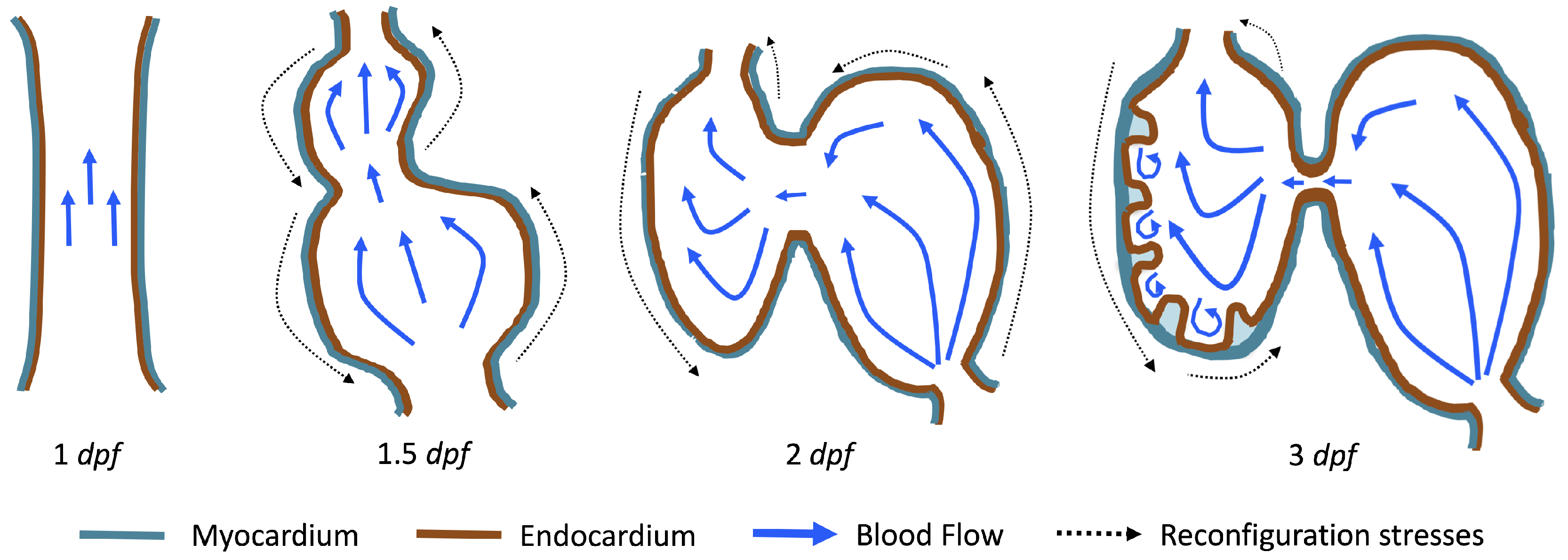
The first heart beat occurs around ∼1 dpf when its morphology resembles a simple valveless tube. It is composed of both an outer myocardial and endocardial layer of cells. Around
dpf cardiac looping and chamber ballooning begins, where the heart drastically begins to reshape itself into a multi-chambered pumping system. Two chambers can be distinctly seen by 2 dpf, while endocardial cushions, the precursors to valve leaflets, are in the process of forming. Trabeculae, irregular muscular protrusions that expand from the inner surface of the ventricle, begin to form around 3 dpf. These stages are illustrated in
Figure 1.
Prior to trabeculation, the endocardial ventricular cells are smooth and polygonal in shape. During the onset of trabeculation, several endocardial cells become elongated and some extend cellular projections. Moreover, these cells appear slightly more depressed than the surrounding endocardial cells. The depressions progressively become deeper and wider such that the endocardial cells invaginate the cardiac jelly and extend toward the basal surface of the myocardium. Eventually, myocardial cells separate due to the potent endocardial cell invasion, and definitive trabeculae are formed [
15]. Hence, trabeculae are composed of both myocardial and endocardium components.
Proper trabeculation requires well-coordinated cardiac contraction [
16] and is particularly sensitive to local changes in the fluid environment [
17]. It is thought that the trabeculae may serve as mechanotranductive structures and alter intracardial flows in a way that regulates shear stress and mixing near the endocardium [
18,
19,
20]. Even if subtle trabeculation irregularities were masked, cardiac defects would magnify over time because of their effect on morphogenetic processes. For example, zebrafish embryos designed to lack normal trabeculation (
ErbB2-inhibited) displayed severe cardiovascular defects including bradycardia (decreased heart rate), decreased fractional shortening, and impaired cardiac conduction [
21]. Lack of trabeculae or irregularly formed trabeculae will cause irregular patterns of shear stresses. This in turn can cause dysfunctional myocardial activation patterns that are known to cause arrhythmias, abnormal fractional shortening, and even ventricullar fibrillation [
22].
During the onset of trabeculation, the underlying fluid dynamics are particularly interesting due to the balance of inertial and viscous forces. The Reynolds number, , is a dimensionless number that describes the ratio of inertial to viscous forces in the fluid. It is given by , where and are the dynamic viscosity and density of embryonic blood, respectively, and L and U are characteristic length and velocity scales. The characteristic velocity is often chosen as the average or peak flow rate, while L is often selected as the diameter of the chamber or vessel. When trabeculation begins as cardiac looping and ballooning progress, the is approximately 1. At this fluid scale, a number of important fluid dynamic transitions can occur. One notable feature is the transition to vortical (disturbed) flow and hence changes in flow direction. This transition is sensitive to the growing complex morphology, effective viscosity of the blood, and unsteadiness of the flow.
Disturbed blood flow patterns have been observed during heart development [
23]. These flow patterns generally induce lower wall shear stresses (WSS) than smoothly streaming (non-disturbed) blood flow. Both contribute to remodelling and endothelial cell activation in different ways [
24,
25]. It has been shown that disturbed (vortical) flow patterns upregulate the expression of certain genes, such as Notch1, in endothelial cells during development [
26]. As the heart undergoes dramatic morphological transformations, transitions to vortical and disturbed flow patterns may help guide morphogenesis through changing patterns in WSS or through other mechanotransductive mechanisms such as flow sensing through primary cilia [
27,
28,
29]. Note that intracardial flows are both temporally and spatially varying such that the distribution of WSS is not uniform along the endothelium [
19,
20]. Hence, mechanotransducers will exhibit different responses, leading to differentiated cellular behavior [
30]. Furthermore, as the heart grows, blood flow also increases [
31]. The formation of complex structures along the ventricle, like trabeculae, may provide regions where disturbed flow develops which could lead to higher kinetic energy dissipation. This energy dissipation may facilitate proper ventricle contractile function and trabecular organization [
20].
Due to the complexity of the cardiogenesis and the challenges of measuring flow patterns precisely, computational fluid dynamics (CFD) has become a premier tool for resolving the flow in embryonic hearts [
19,
20,
32,
33,
34,
35,
36,
37,
38,
39,
40,
41]. For example, Liu et al. [
34] simulated flow through a three-dimensional model of a chick embryonic heart during stage HH21 (after about 3.5 days of incubation) at a maximum
of about 6.9. They found that vortices formed during the ejection phase near the inner curvature of the outflow tract. In 2013, Lee et al. [
38] performed 2D simulations of the developing zebrafish heart with moving cardiac walls. They found that unsteady vortices develop during atrial relaxation at 20–30 hpf and in both the atrium and ventricle at 110–120 hpf.
More recently, Vedula et al. [
19] and Lee et al. [
20] used light-sheet fluorescent microscopy and reconstructed a
moving ventricle on which they based their CFD model. They were able to quantify spatially- and temporally-varying WSS along trabceular ridges (trabeculae “heads”) and groves (“intertrabecular regions”). In particular, Lee et al. discovered that pulsatile shear-stresses developed along the ridges at 3 dpf in wildtype (WT) zebrafish embryos, while oscillatory shear-stresses (OSS) developed in the groves around 4 dpf [
20]. Around 4 dpf, vortical flow patterns may be present within the intertrabecular spaces. Moreover, OSS were found to be substantially less at the trabecular heads, suggesting that OSS may be a possible regulatory control during cardiogenesis [
19,
20]. They also investigated differences in WSS between wildtype and mutant zebrafish hearts. The mutants they considered were
ErbB2-inhibited zebrafish (suppresses trabeculation),
gata1a morpholinos (lowers blood viscosity), and
wea mutants (lower cardiac contractility). They found that total WSS was comparable in the WT and ErbB2-inhibited zebrafish; however, the
gata1a morpholinos and
wea mutants expressed significantly less total WSS. Another study, Battista et al. [
40], found that trabeculae morphology has a significant effect on intertrabecular vortex formation, as does the presence of hematocrit and fluid scale. However, their study did not include an analysis of WSS, but instead referred to the tangential, normal, and total force magnitudes as potential proxies for WSS, although they observed similar trends to the spatially-averaged WSS over the course of a heart cycle.
The numerical work described above and in vivo measurements of blood flow in embryonic hearts [
3,
42] supports that vortex formation is sensitive to changes in
, morphology, and unsteadiness of the flow. Santhanakrishnan et al. [
35] used a combination of CFD and flow visualization in dynamically scaled physical models to describe the fluid dynamic transitions that occur as the chambers balloon, the endocardial cushions grow, and the overall scale of the heart increases. They found that the formation of intracardial vortices depends upon the height of the endocardial cushions, the depth of the chambers, and the
. Their study only considered steady flows in an idealized two-dimensional chamber geometry with smooth, stationary walls.
In this paper, we present complementary studies to both Santhanakrishnan et al. [
35] and Lee et al. [
20] with the goal of revealing the bifurcations in flow structures that occur as a result of the unsteadiness of the flow, trabeculae height, and
. First, we investigate the differences in the cardiac fluid dynamics between WT and
ErbB2-inhibited (namely
ErbB2 and
ErbB2) mutants, to explore how vortex formation in the intertrabecular regions is sensitive to differences in morphology. We quantify the intertrabecular flow patterns mentioned (but not shown) in Lee et al. [
20]. Next, we use an idealized geometry, based upon that of Santhanakrishnan et al. [
35], to systematically sweep a parameter space consisting of trabeculae size, fluid scale, and unsteady flow effects to quantify fluid dynamics transitions.
It is important to note that, in this study, we perform 2D simulations using stationary boundaries. This permits direct comparison to the steady flows moved through the simplified chambers considered by Santhanakrishnan et al. [
35]. It also permits exploration of a wide parameter space that covers the range of biological diversity, including other trabeculated vertebrate embryonic hearts and trabeculated invertebrate hearts. As such, the results highlight parameter spaces where bulk flow patterns are highly sensitive to small changes in morphology, effective viscosity, and unsteadiness of the fluid. In such parameter regions, it is critical to obtain highly resolved descriptions of morphology, pumping kinematics, and rheology of the blood. The simulation results shown here are not as realistic as those presented for the zebrafish embryonic hearts simulated in 3D with moving boundaries by Lee et al. [
20] and Vedula et al. [
19]. Our goal, however, was to map the parameter space sensitive to small changes in a relatively simple model. We believe that the results will serve as motivation for more detailed three-dimensional studies. We also argue that the stationary boundaries and 2D approximations serve as a reasonable starting point given the relatively low Womersley number,
, since unsteady effects become significant for
.
3. Results
Below, we present the flow patterns and velocities for both biologically realistic and idealized models of trabeculated ventricles. The cases with biologically realistic geometries were of WT zebrafish and an ErbB2-inhibited mutant to contrast the intracardial and intertrabecular fluid dynamics of an embryonic zebrafish heart during development. The idealized geometry was used to systematically sweep over a parameter space to describe transitions in flow patterns for pulsatile flows, changes in trabecular height, and Reynolds Number . In the idealized geometry case, the was varied from 0.01 to 100, and the trabecular heights were varied from zero to twice the biologically relevant height. We also quantified flow for both steady and pulsatile cases.
Streamlines were used to show the path that a passive particle would take in the flow. The streamline graphs were generated using the VisIt visualization software (v. 2.7.2, Lawrence Livermore National Laboratory, Livermore, CA, USA) [
47]. The streamlines are drawn by making a contour map of the stream function, since the stream function is constant along the streamline. The stream function,
, in 2-D is defined by the following equations:
The streamline colors correspond to smooth, streaming flow (blue) and vortical flow (orange).
3.1. Steady Flow through an Embryonic Zebrafish Heart
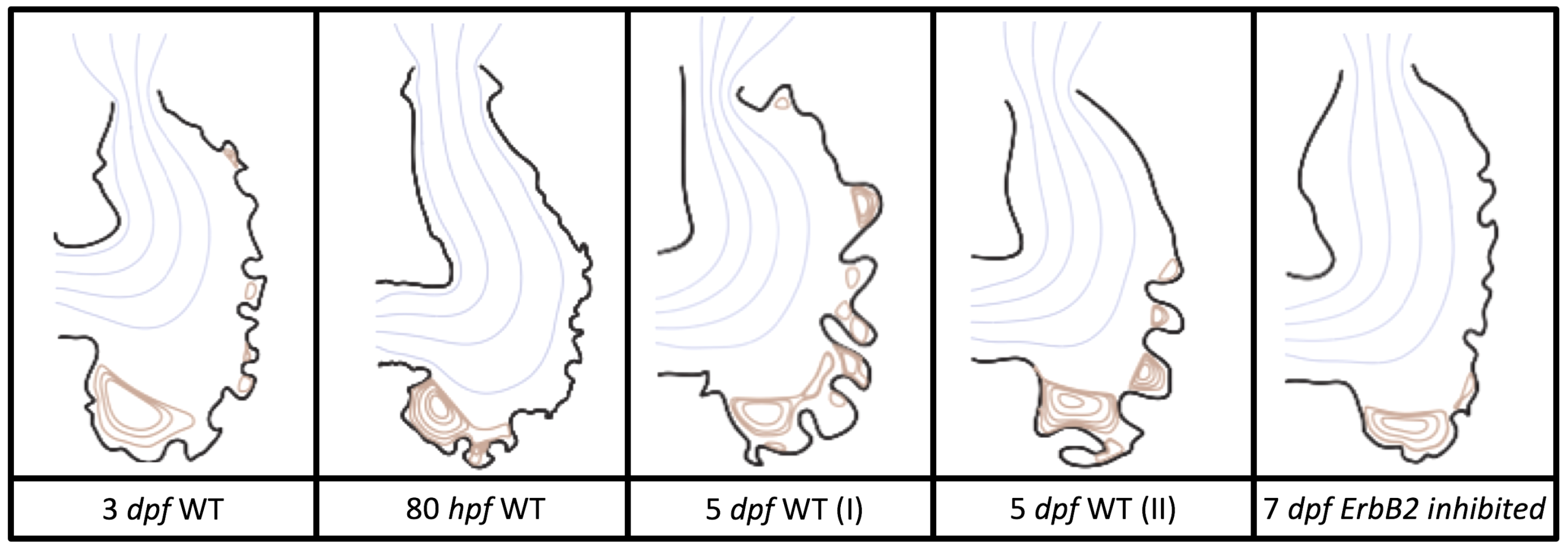
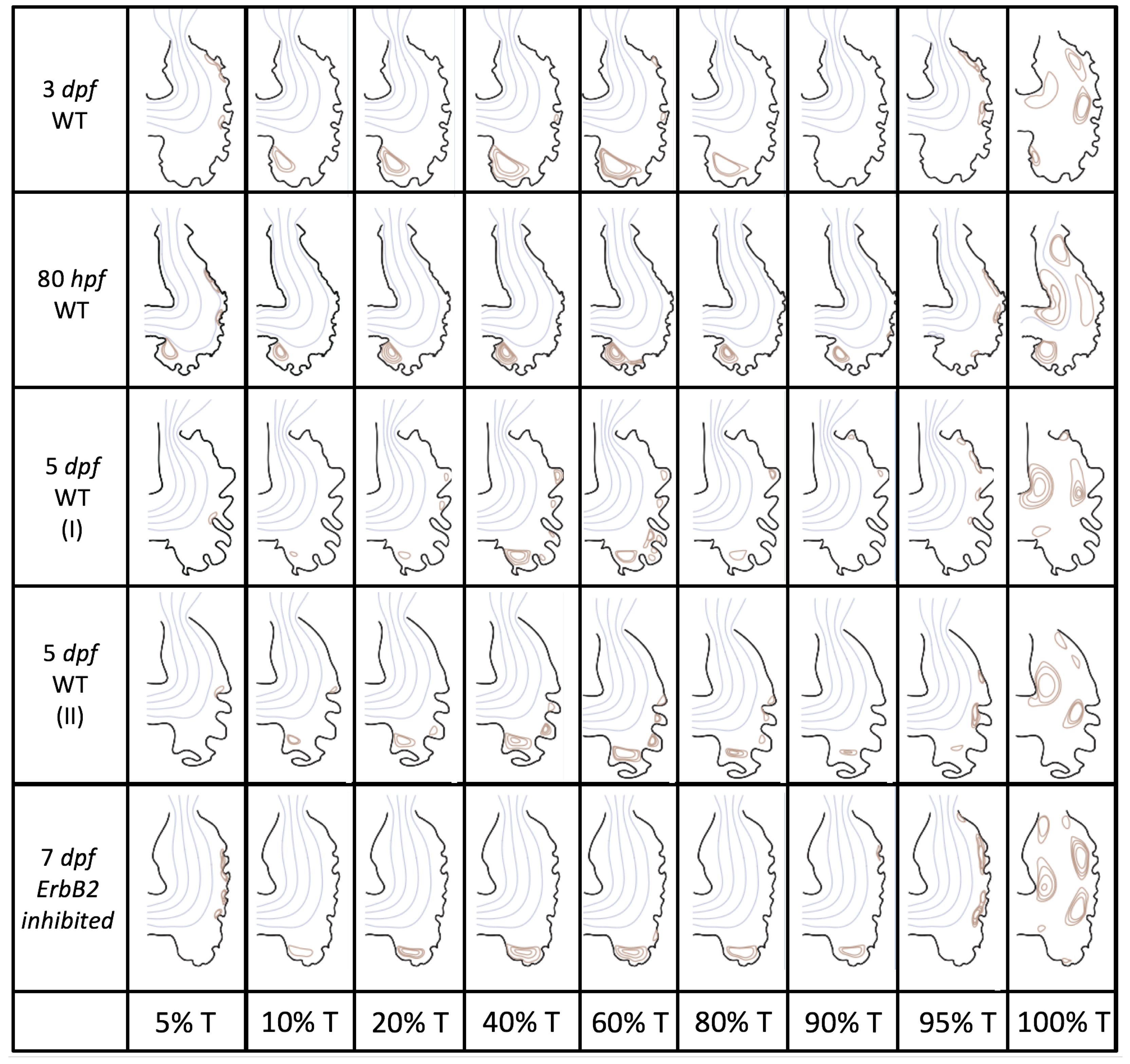
Figure 5 gives the flow field streamlines for the steady inflow cases with biologically realistic geometries at
. Parabolic inflow was used that accelerates from rest to a constant velocity, as detailed in
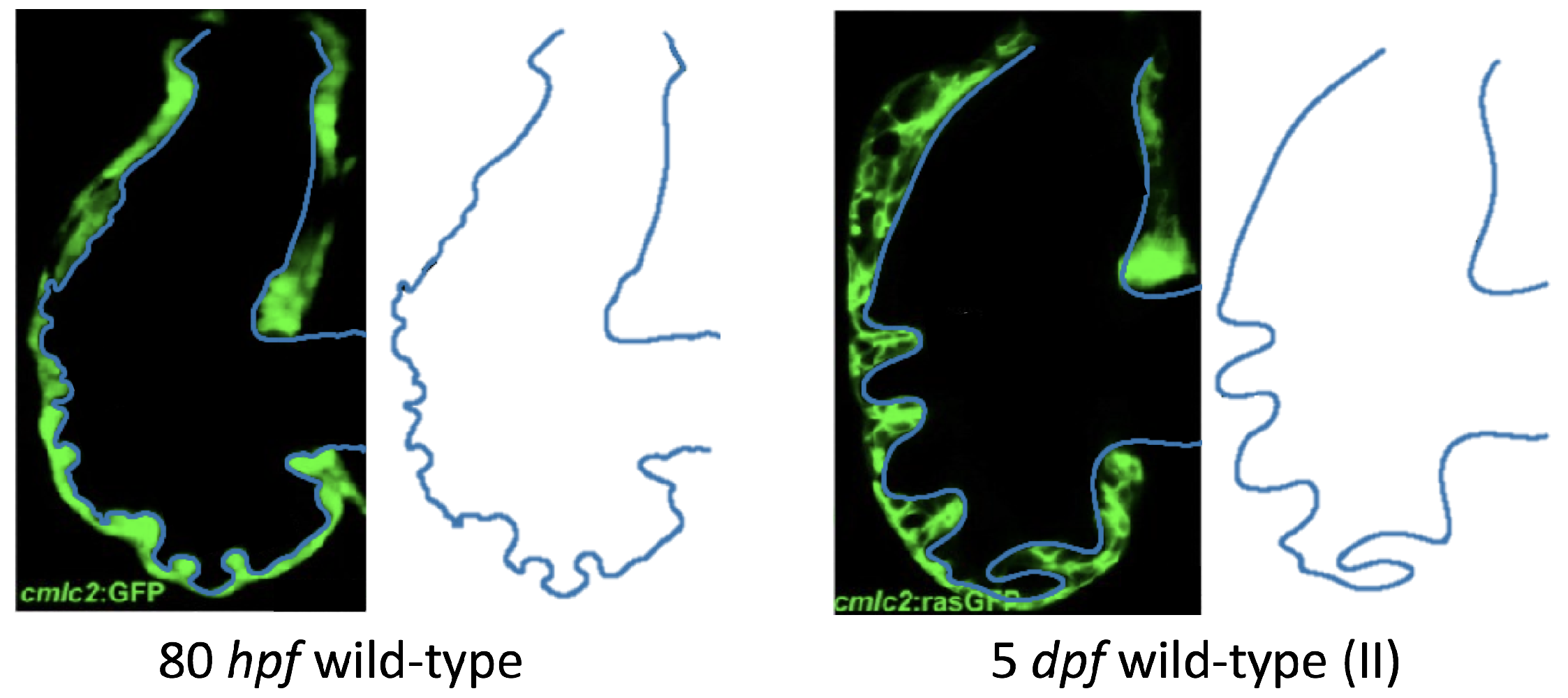
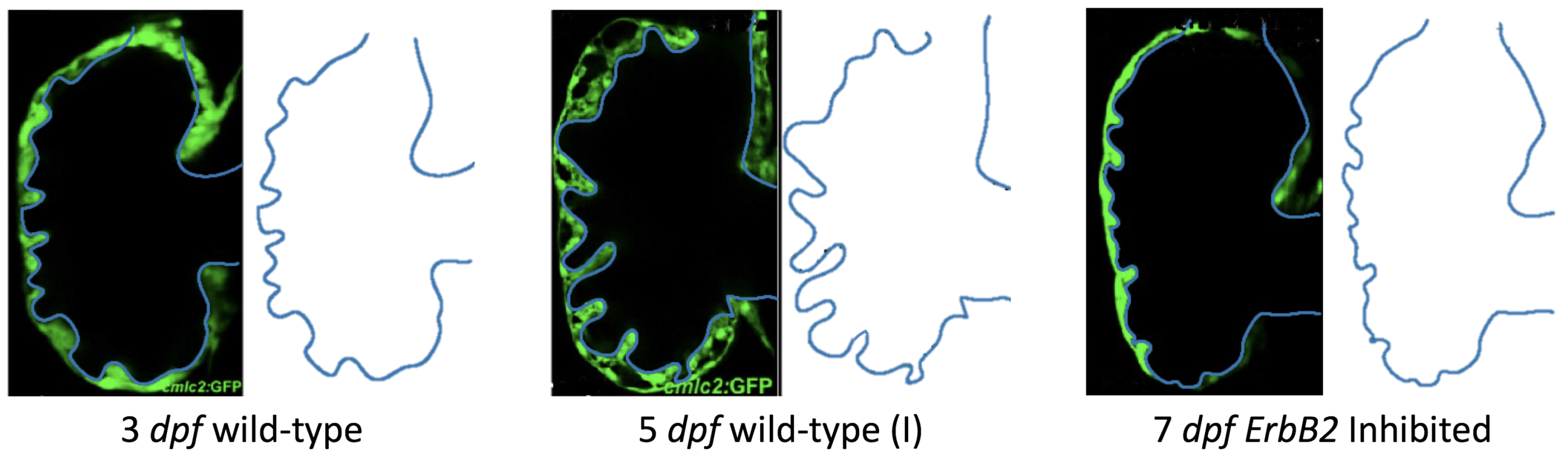
Appendix A. The simulation data is given once the flow has reached its steady state. Results are shown for a 3 dpf, 80 hpf, and two 5 dpf wild-type embryos as well as an
ErbB2-inhibited embryo at 7 dpf. In all cases, vortex formation occurred in the intertrabecular regions along the side opposite that to the sinus venosus (SV) and was within the well pronounced intertrabecular grooves. No intracardial vortices were observed and the flow smoothly steams from the atrioventricular canal to the sinus venosus.
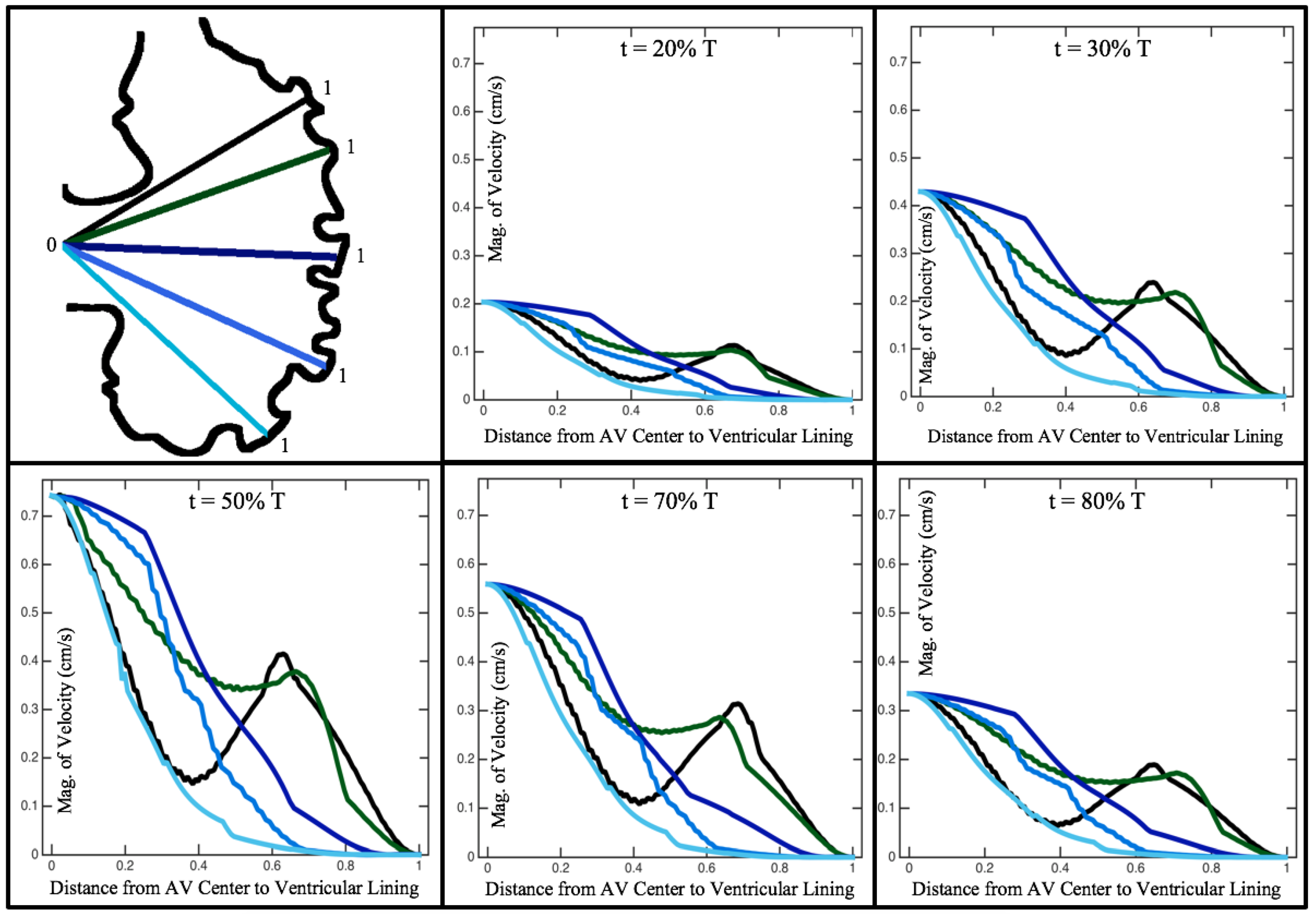
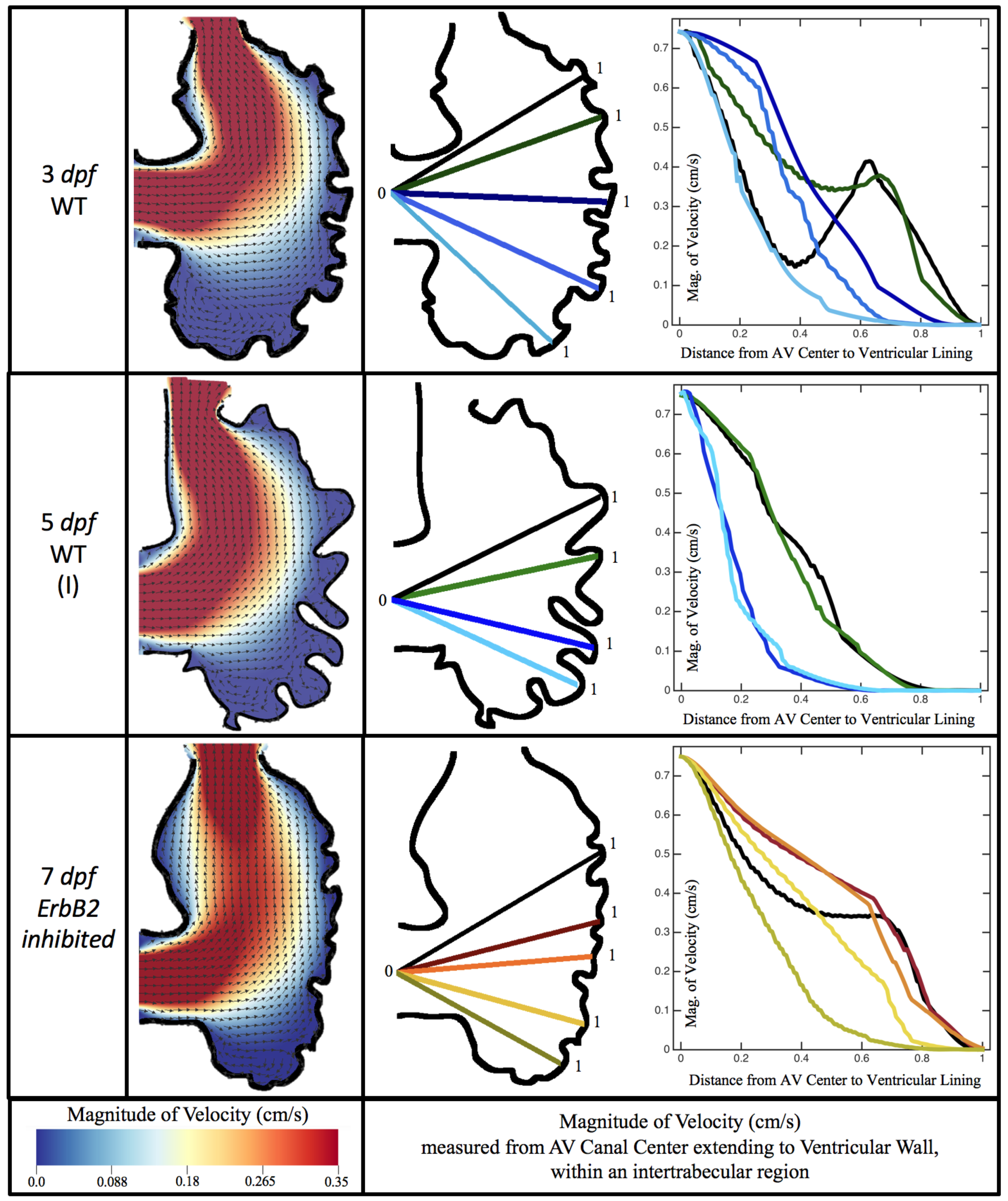
Figure 6 illustrates that, in the regions of significant vortex formation, e.g., in the intertrabecular regions, velocities are much lower than in the intracardial region of the ventricle. In all cases, the velocities on the side opposite the SV experience much faster velocity decay towards the ventricular lining, whereas regions opposite the AV canal experience slower decay. Note that, in the 3 dpf and 7
dpf ErbB2 inhibited cases, the flow velocities along the line drawn from the AV canal to the intertrabecular region that is closest to the SV decrease in magnitude before increasing again and finally decaying to zero near the cardiac wall. This is due to the fact that the velocity is measured close to the ventricular wall that extends from the AV canal. Flow velocities measured between the trabeculae are significantly lower than those measured in within the middle of the chamber.
3.2. Pulsatile Flow through an Embryonic Zebrafish Heart
In this subsection, we show the results of the pulsatile inflow simulations where biologically realistic geometries are used at
and the frequencies are varied. Temporal snapshots of the streamlines are presented in
Figure 7. The pulsatile inflow condition is detailed in
Appendix A. Note that the period of the pulsation cycle is
T. At the beginning and end of each pulsatile cycle, the flow is near zero. During the middle of the pulsation cycle, flow is maximal. Although this model is an idealization, we consider the first 50%
T as analogous to diastole and 50–100%
T as systole. All data shown is taken from the last pulse cycle such that periodic steady state has been reached. The geometries simulated include a 3 dpf, a 80 hpf, and two 5 dpf wild-type embryos as well as an
ErbB2 inhibited embryo at 7 dpf.
Vortices formed in all cases within the intertrabecular regions along the side opposite that to the sinus venosus, similar to the steady cases illustrated in
Figure 5. The vortices are, however, dynamic; they change shape and size during a single pulsation cycle. Some additional vortices appear in the intertrabecular regions that were not present in the steady case. For example, consider the 80 hpf and
ErbB2-inhibited cases where vortices appear on the side opposite the AV canal. Furthermore, large intracardial vortices appear between pulsation cycles in all cases when there is minimal inflow.
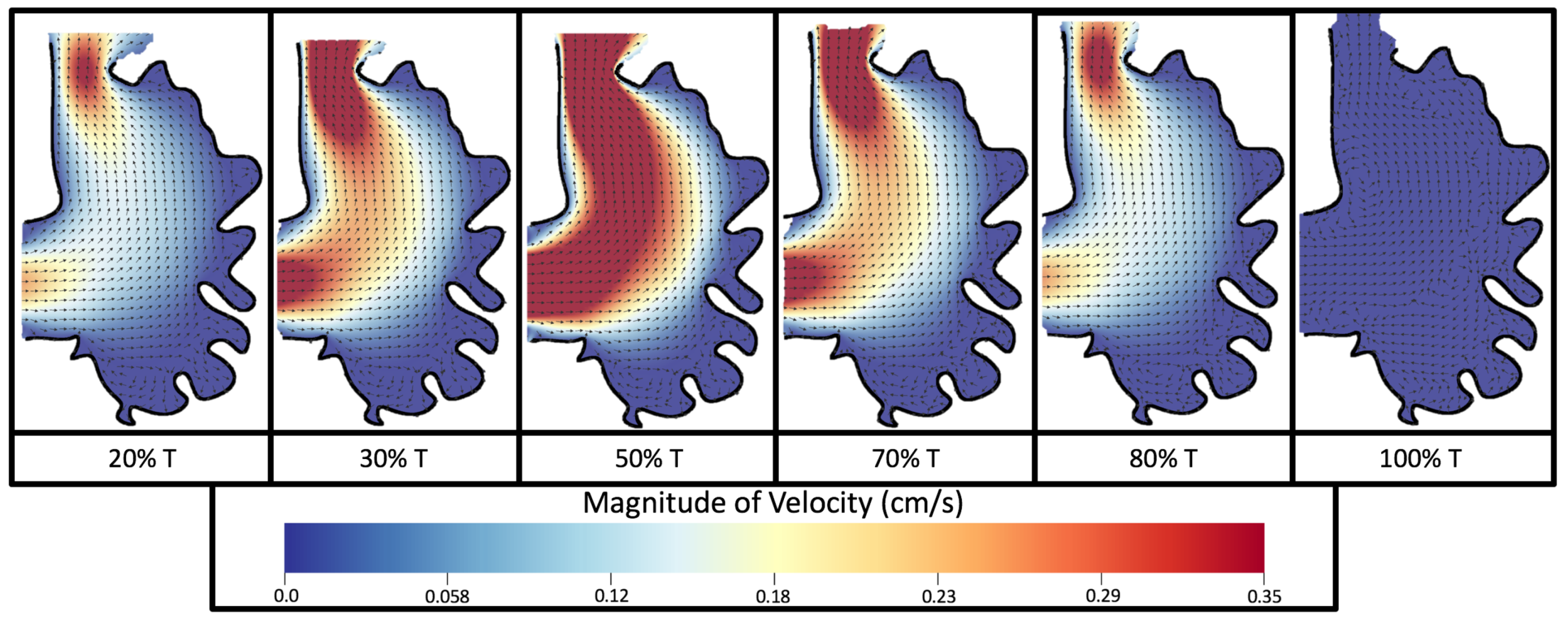
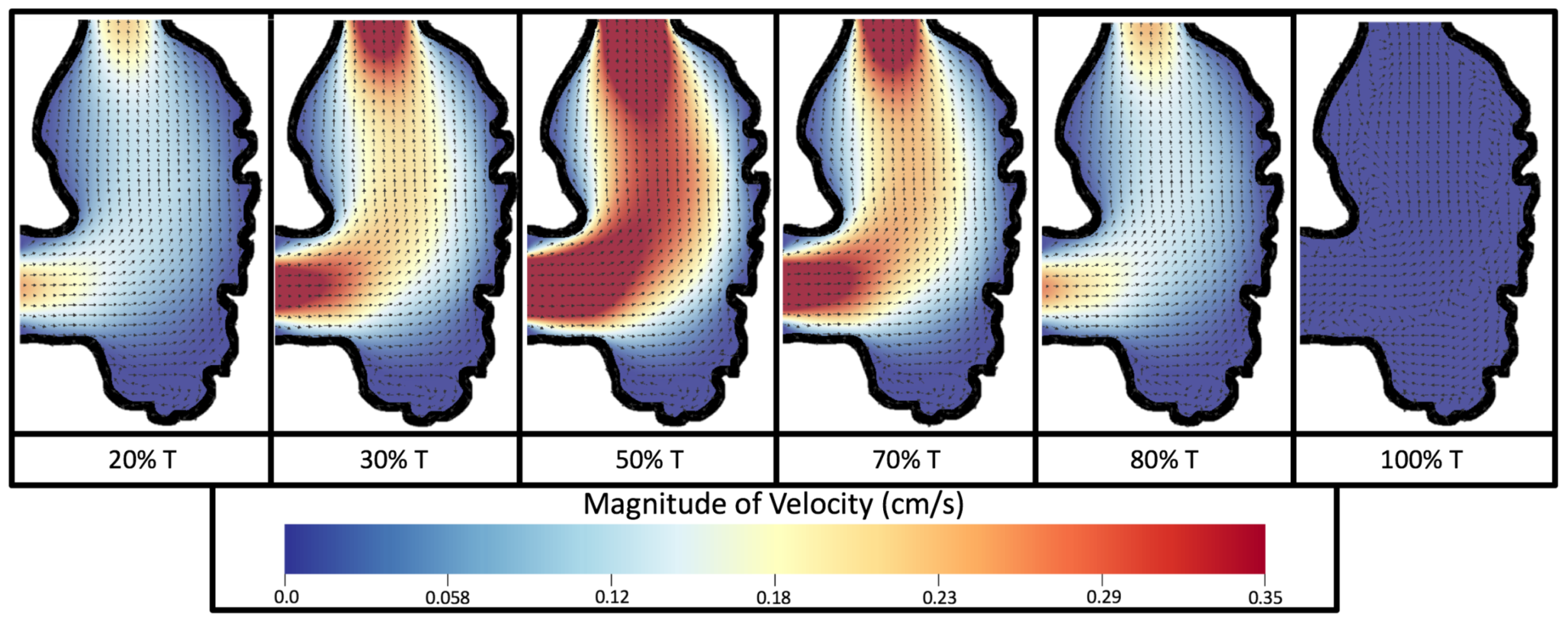
Figure 8 and
Figure 9 give temporal snapshots for the 5 dpf WT (I) and the
ErbB2-inhibited cases, respectively. The colormap illustrates the magnitude of velocity (cm/s) with accompanying velocity vector fields. The velocity field is consistent with
Figure 7 and shows vortex formation. These results also illustrate the spatial gradient in velocity within the intracardial to intertrabecular regions. It is clear that, although the fastest flow moves towards the middle of the chamber, the velocity significantly tapers off by the time it reaches the ventricular lining, the region between trabeculae on the right-hand side of the ventricular geometries in
Figure 8 and
Figure 9.
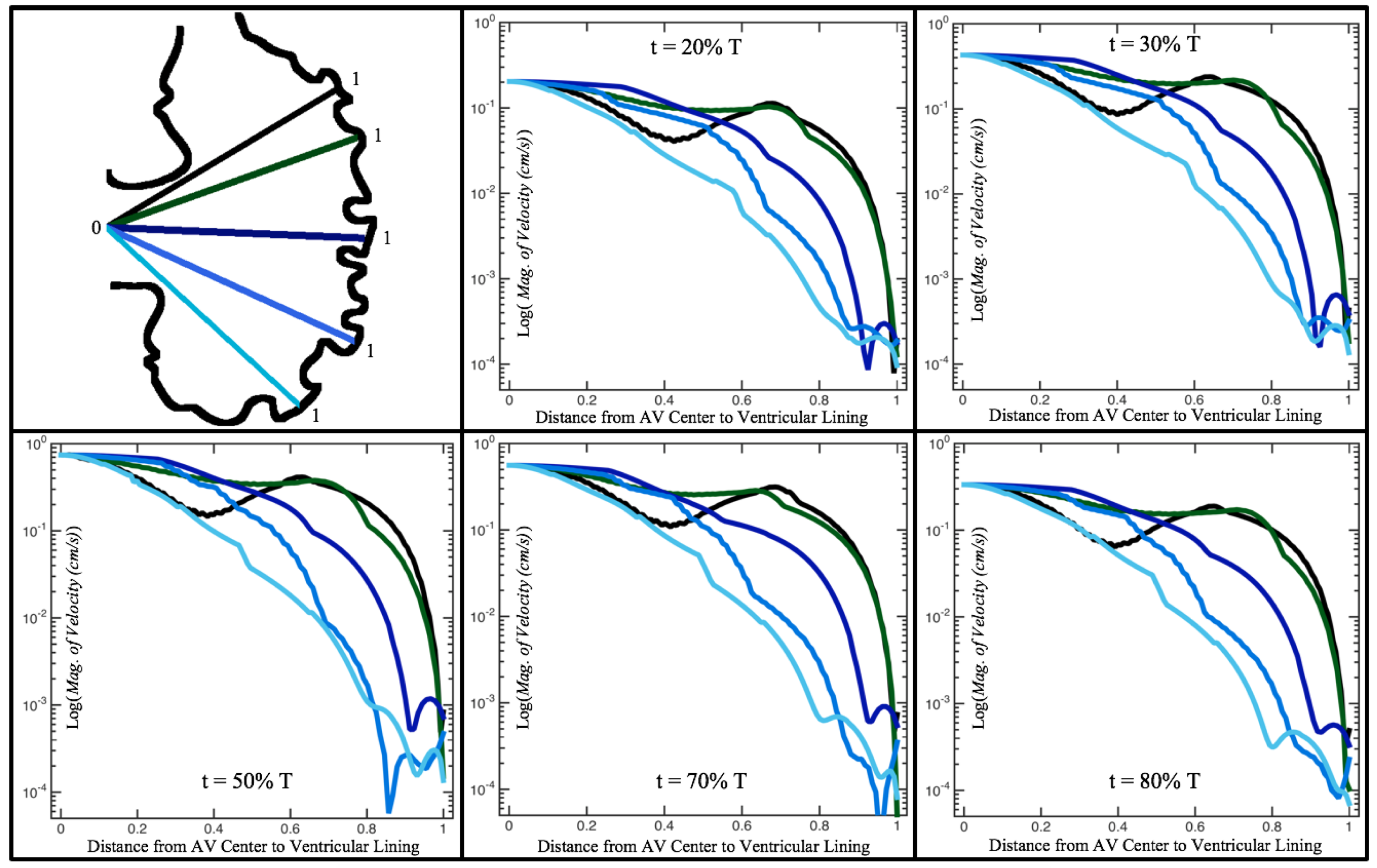
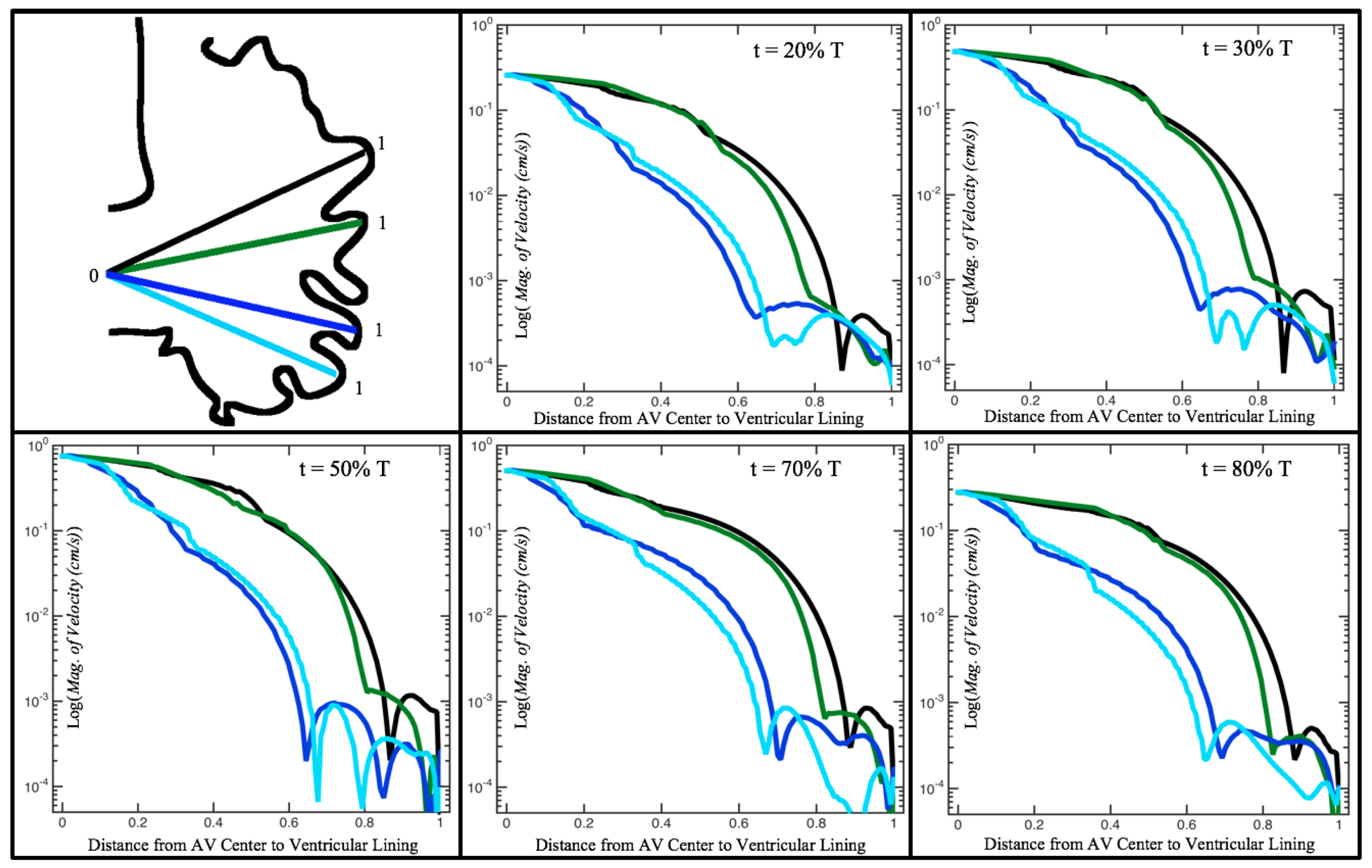
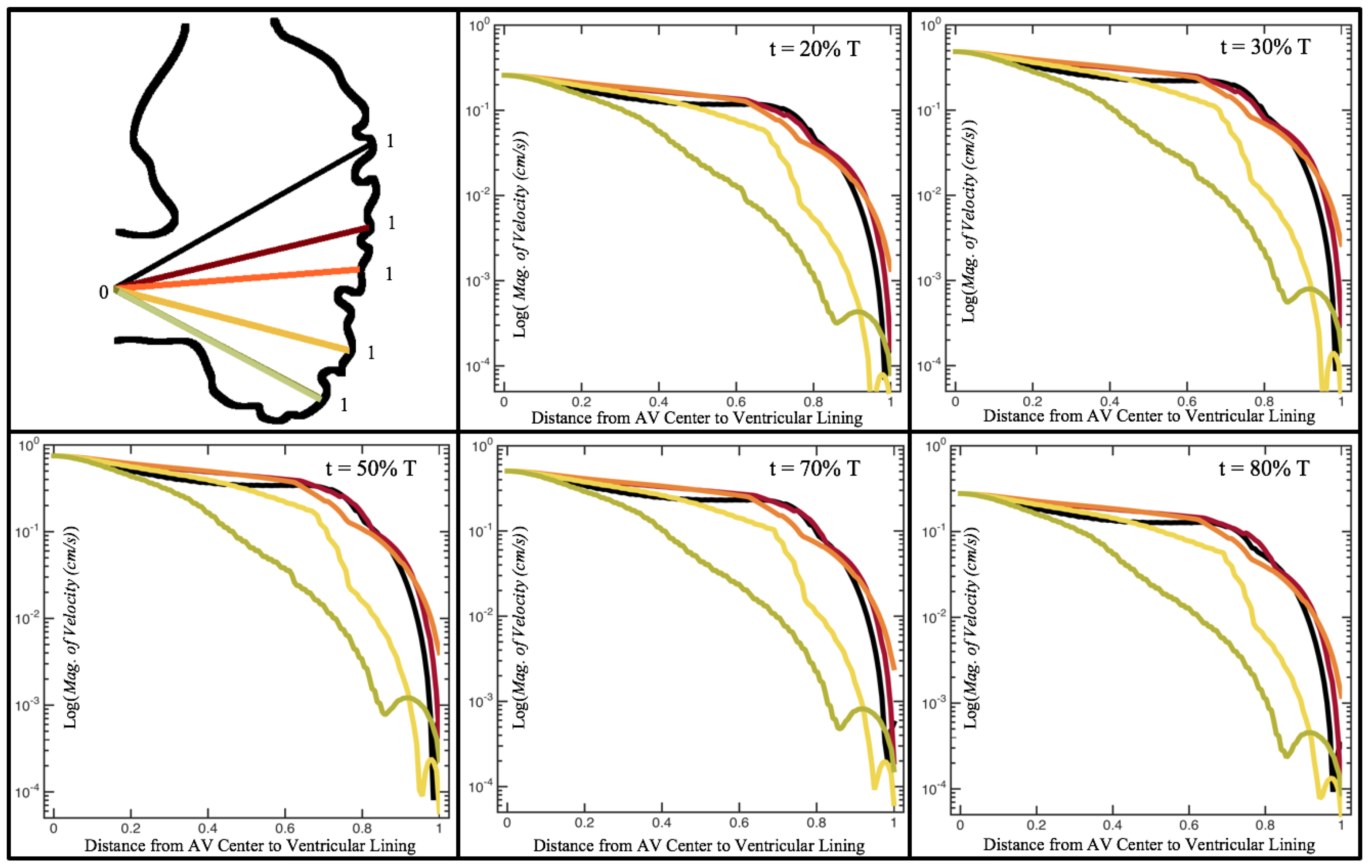
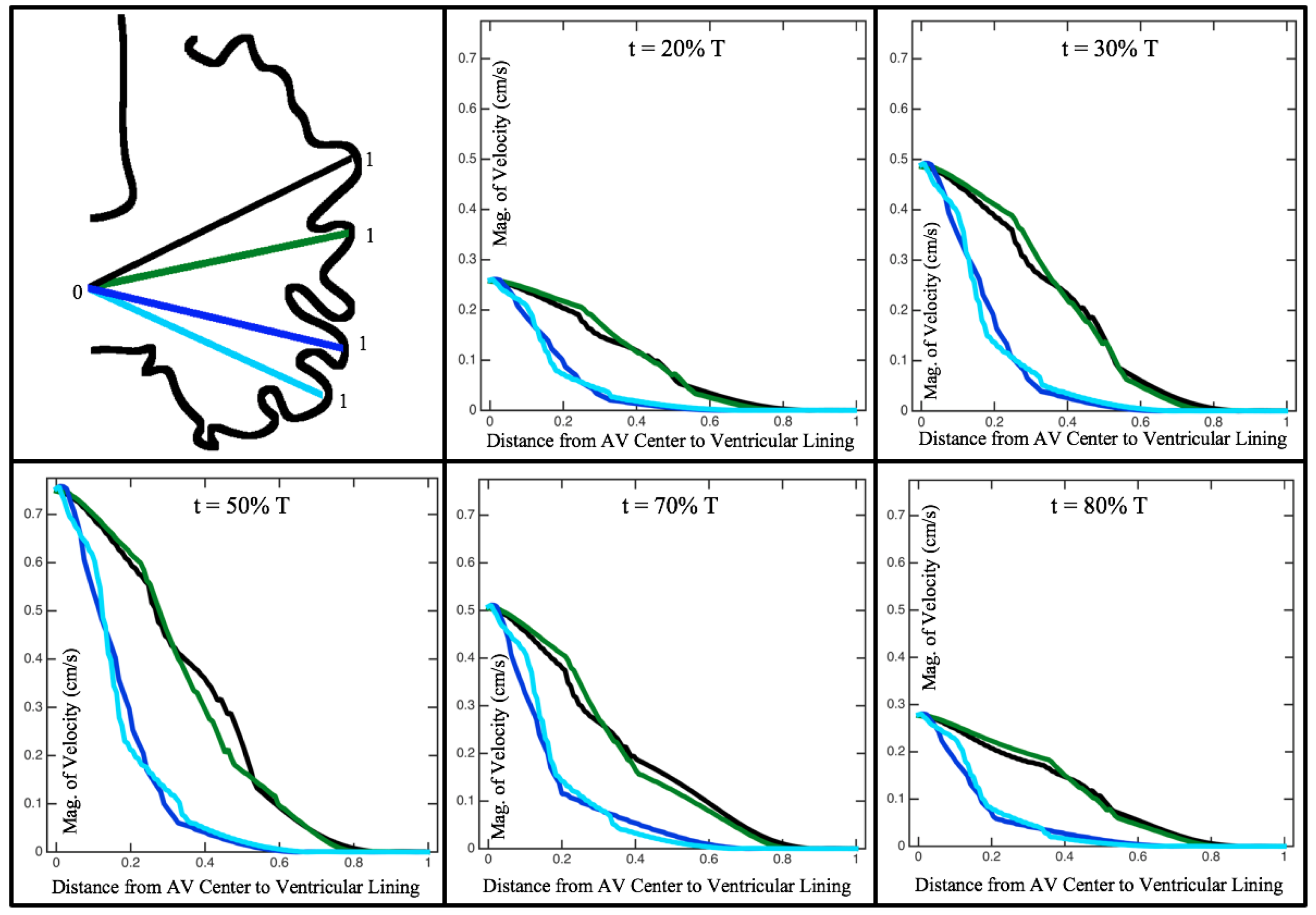
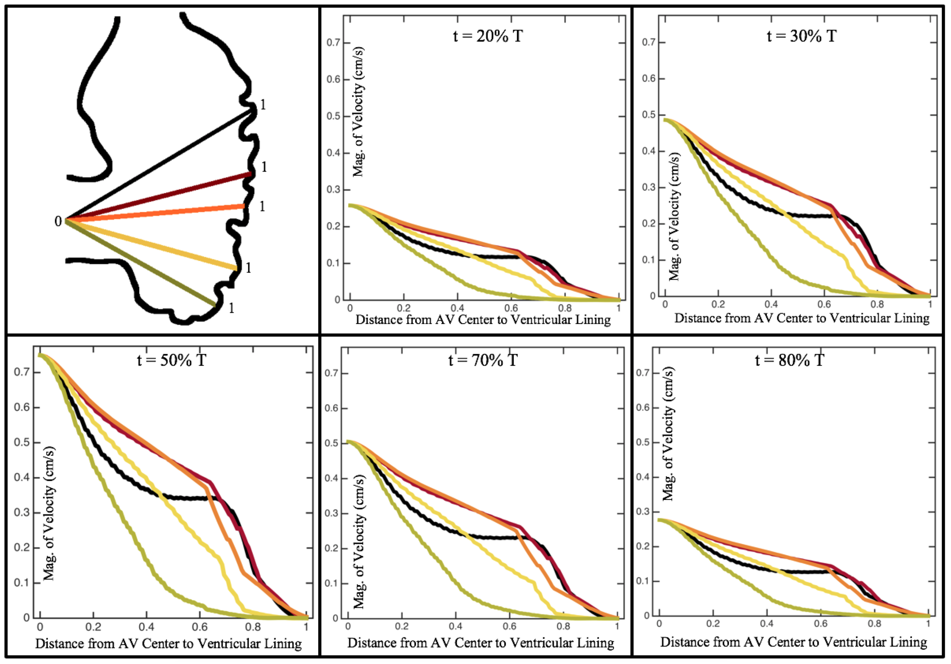
Figure 10,
Figure 11 and
Figure 12 illustrate the magnitude of the velocity along lines drawn from the center of the AV canal to the intertrabecular regions for cases of a 3 and 5 dpf WT (I) and 7
dpf ErbB2-inhibited zebrafish geometries.
Appendix C presents this data in a non-logarithmic scale, to complement the data given in
Figure 6 in
Section 3.1. Note that the 3 dpf WT and 7
dpf ErbB2-inhibited zebrafish exhibit smaller trabeculae than the 5 dpf WT (I) case.
As expected in all cases, peak flows occur within the chamber and decay as one moves toward the cardiac wall. Even in the steady inflow cases, the velocity decay is similar. The velocity decreases close to geometrically towards the intertrabecular region on the opposite side to the SV for the smaller trabeculae (3 dpf WT and 7 dpf ErbB2-inhibited). For the 3 dpf WT embryos in regions with pronounced trabeculation, the velocity decay does not monotonically decrease; it increases slightly within the trabeculae before decreasing to zero as one moves towards the endocardium. Similar non-monotonic behavior is seen for some intertrabecular regions farther from the SV in the 3 dpf WT and 7 dpf ErbB2-inhibited embryos. We also note that the magnitude of flow decreases much more rapidly for the 5 dpf WT (I) with pronounced trabeculation, indicating lower WSS within the intertrabecular regions.
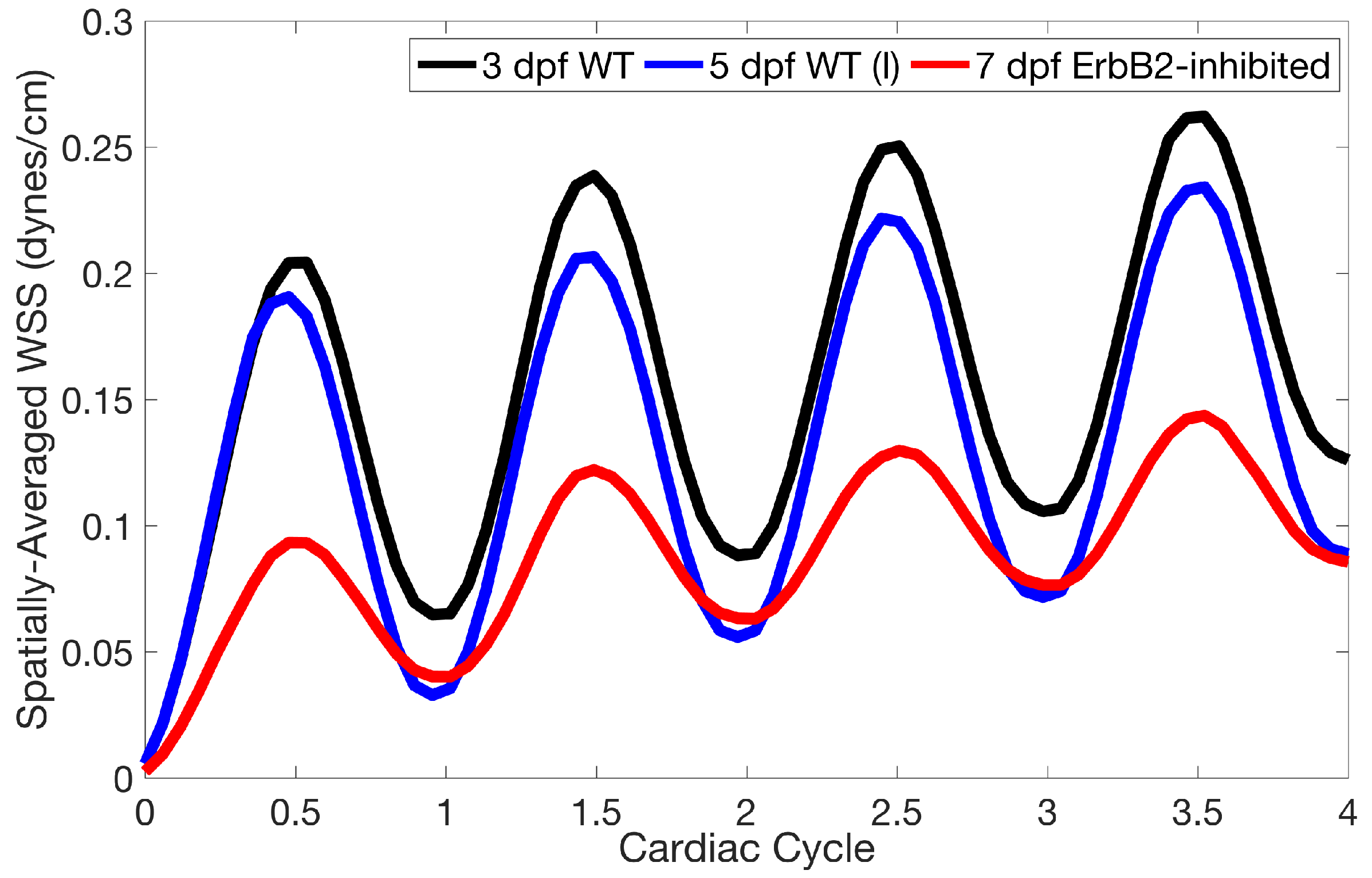
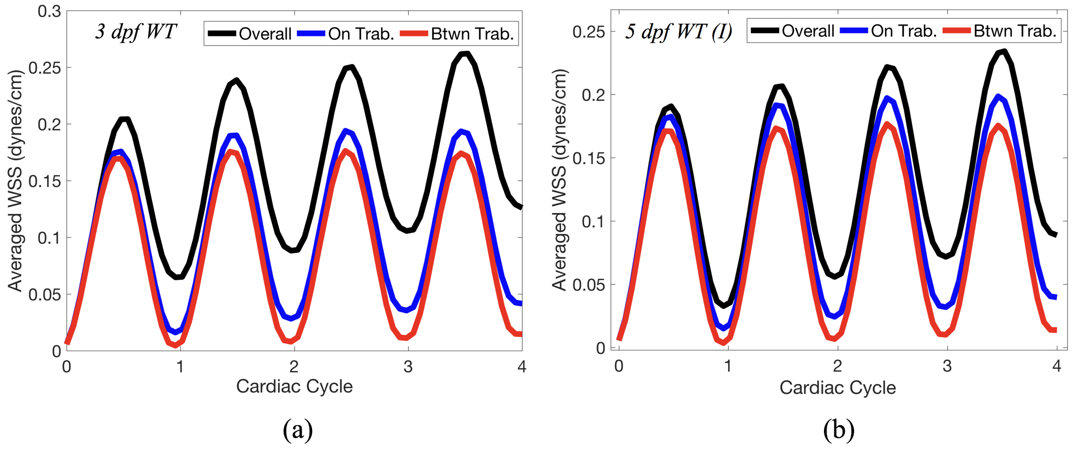
Lastly for the case of pulsatile flow through realistic geometries, we computed the spatially-averaged wall shear stress (WSS) over the entire ventricular geometry, each pronounced trabeculae, and intertrabecular region, see
Figure 13, as well as the oscillatory shear index (OSI). The OSI is a dimensionless metric of how aligned the WSS vector is with the time-averaged WSS (TAWSS) vector throughout one cardiac cycle. Recently, it has been suggested to be a possible regulatory mechanism of trabeculation itself [
19]. Details regarding how WSS, TAWSS, and OSI were calculated can be found in
Appendix D.
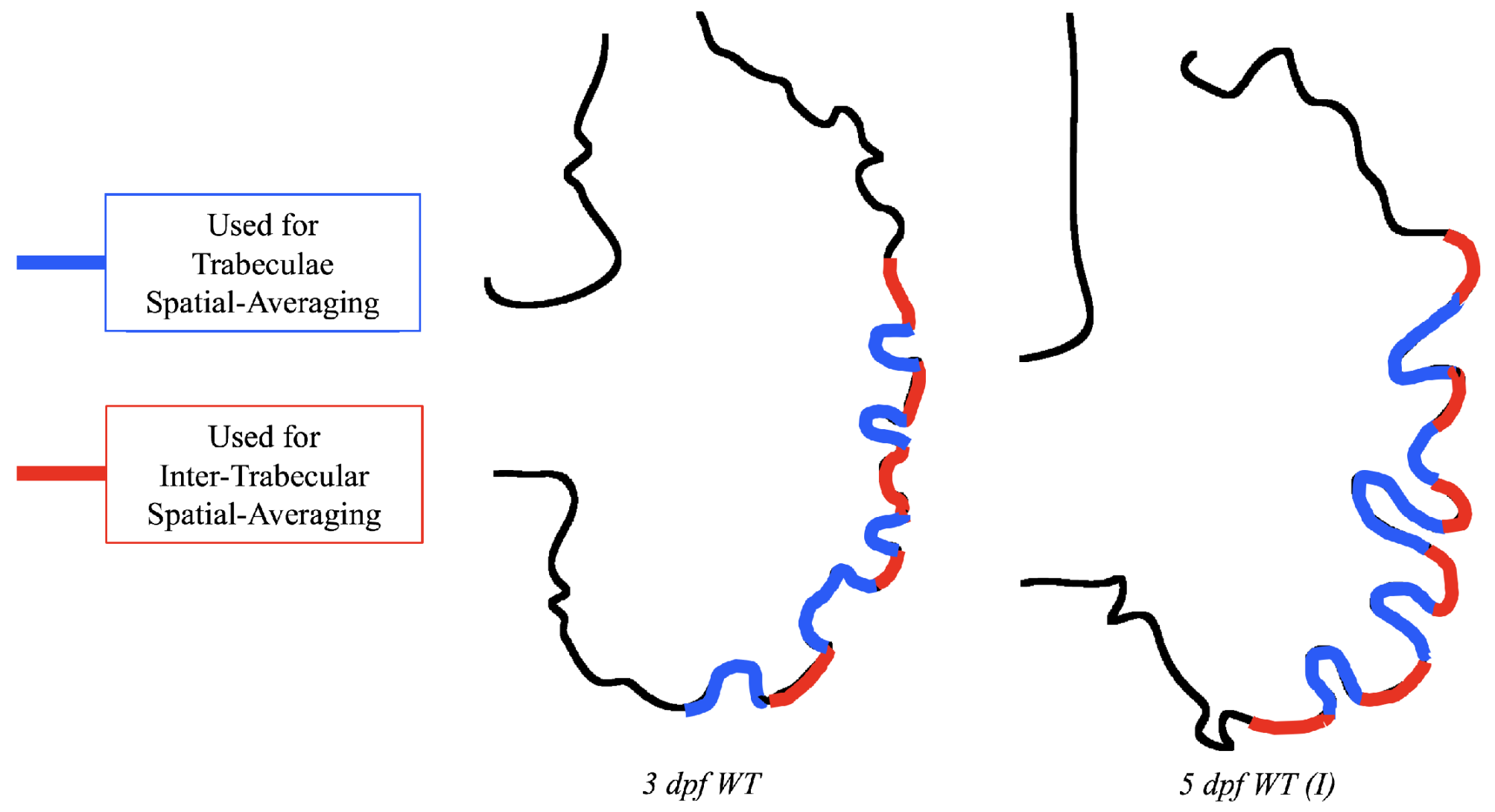
Figure 14 gives spatially-averaged magnitude of WSS over the trabeculae, intertrabecular regions, and entire ventricle for the 3 dpf WT and 5 dpf WT (I) zebrafish geometries. The intertrabecular regions experience slightly less (∼10%) less spatially-averaged WSS than pronounced trabeculae. The majority of the WSS is felt elsewhere within the ventricle, e.g., near the AV-canal and outflow tract. See
Appendix D.1 for a description of which trabeculae and intertrabecular regions were used for the analysis.
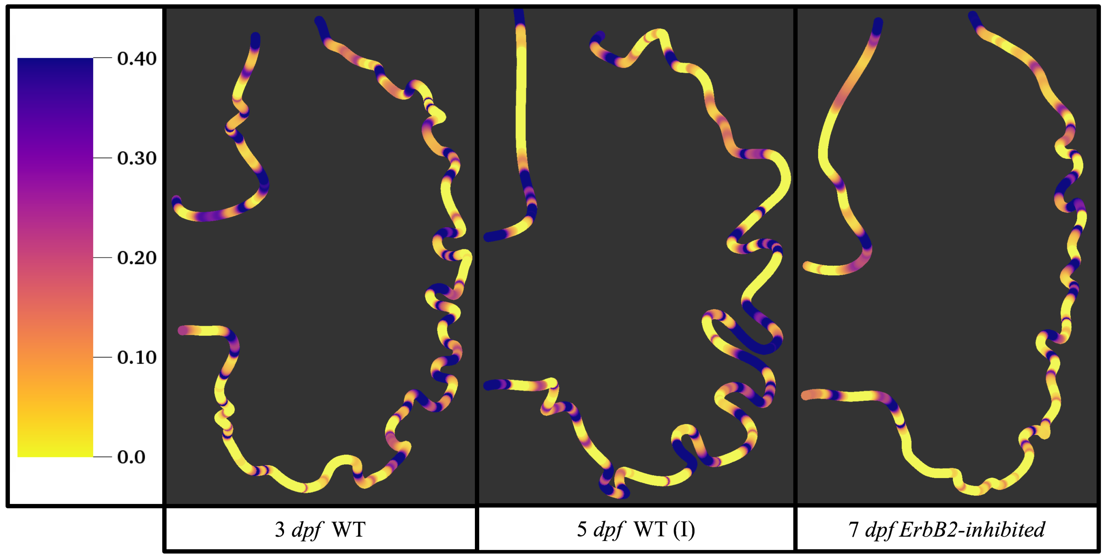
Figure 15 gives the OSI over the entire trabeculated ventricle for the 3 dpf WT, 5 dpf WT (I), and 7
dpf ErbB2-inhibited zebrafish geometries. High OSI
occur in both intertrabecular regions and on the trabeulae themselves. This is similar behavior to [
19,
20] who reported high OSI values in intertrabecular regions as well; however, in our simulations, not all intertrabecular regions nor trabeculae have high OSI. In particular, those nearing the outflow tract (top of geometry) experience less OSI versus those opposite the lower end of the AV canal.
3.3. Steady Flow through Idealized Trabeculated Chambers
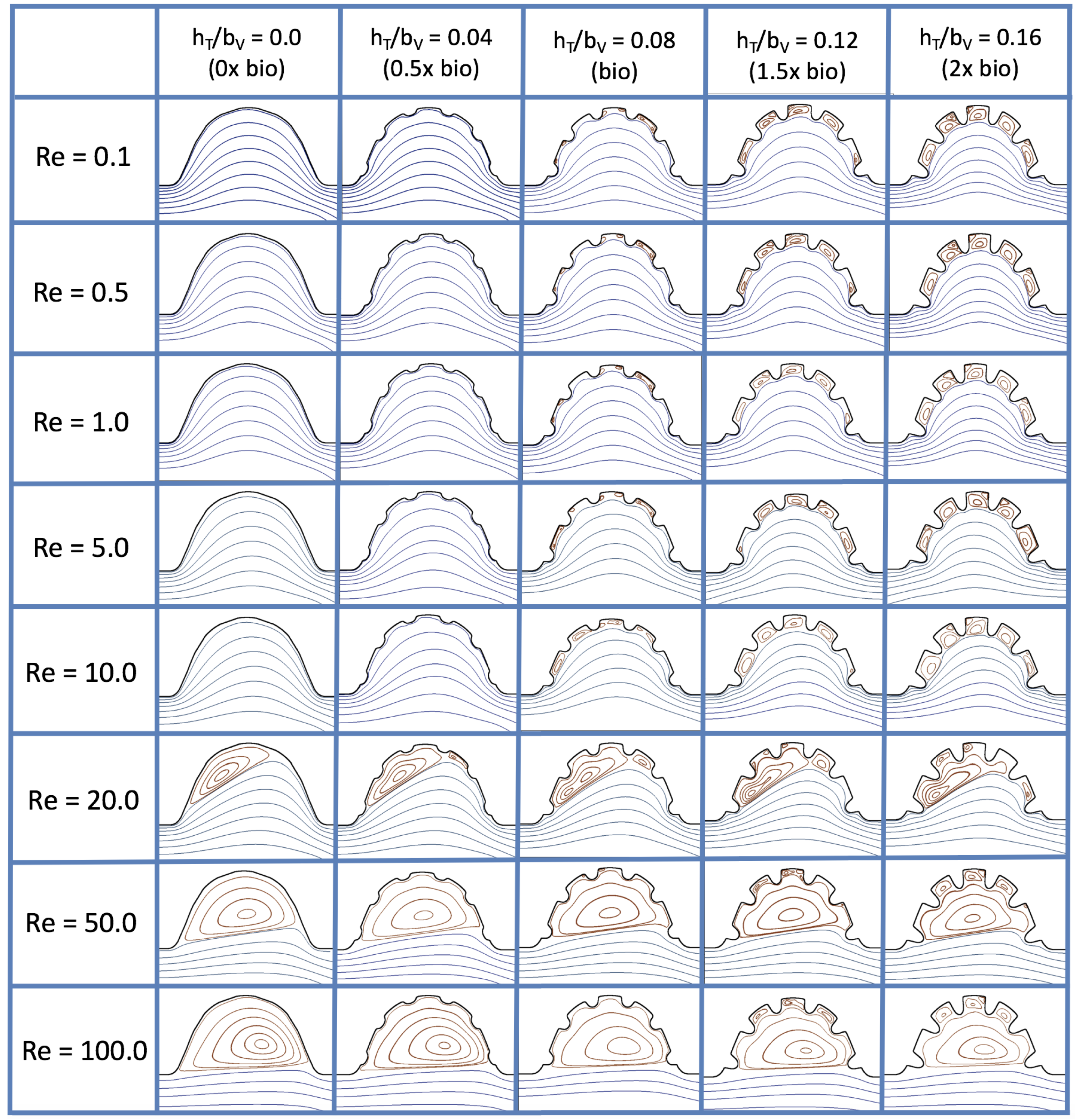
Figure 16 shows the flow field streamlines for the case of steady flow through an idealized trabeculated embryonic ventricle. The inflow condition is detailed in
Appendix A. The numerical simulations span five orders of magnitude of
, varying from 0.01 to 100, while trabeculae heights were set to
. Note that the biologically relevant case is
In the case of no trabeculae (left column), we find vortex formation only occurs for
, in agreement with the findings of [
35]. Moreover, this result appears consistent with fluid dynamics literature on transitions to vortical flow via a channel with an expanded region [
48,
49]. Shen et al. [
48] and Mizushima et al. [
49] both use rectangular cavities; however, similar transitions to vortical flow occur at consistent
. For
, the flow bends around the cavity and no flow separation occurs, that is, there are no transitions to vortical flow patterns. Hence, fluid mixing is not enhanced at for
and flow reversal does not occur. As
is increased to 20, flow reversal occurs and a closed vortex is present along the left side of the cavity. The stagnation point is located between the orange and blue streamlines. To the left of this stagnation point, the flow moves along the endocardium from the right to left. To the right of the stagnation point, the flow moves right to left. As
is further increased, the stagnation point moves to the right, and the intracardial vortex becomes larger until it becomes as large as the cavity itself for
.
When half-size biologically relevant trabeculae are introduced into the model (), similar flow fields emerge for the case of . Although geometric perturbations now exist along the cavity lining, no flow separation occurs, whether intracardially or intertrabecularly, illustrating no vortical flow patterns nor enhanced fluid mixing at these trabeculae heights for . For , we see a similar intracardial vortex to the case without trabeculae; however, this vortex weaves along regions with trabeculae. Furthermore, there is an emergence of an independent closed vortex along the right side between two trabeculae. For , we find the presence of one large intracardial vortex wrapping around each trabeculae.
For biologically relevant trabeculae heights, there are closed intertrabecular vortices for
as low as 0.1, while no intracardial vortices are present at these lower
. Shen et al. [
48] saw a similar phenomenon with the formation of two vortices in the corners of their rectangular cavity. This is consistent with the formation of vortices near the only bottom of the trabeculae. On the other hand, interestingly, not all intertrabecular regions have closed vortices. As
is further increased from
to
, the intertrabecular vortices grow in size. As in previous cases, a larger intracardial vortex forms at
. On the left hand side of the cavity, there is smooth flow from left to right around the trabeculae. On the right side of the cavity, independent closed vortices form between the trabeculae, and the flow is from right to left. For
, a large intracardial vortex forms and no intertrabecular vortices persist.
For trabeculae heights higher than the biologically relevant range, there exist intertrabecular vortices for as low as ; however, compared to the previous biologically relevant case, there are vortices between every adjacent pair of trabeculae. Moreover, because the trabeculae extend further into the ventricular cavity, these vortices are larger than in previous cases. Intracardial vortices do not develop until , where there is the presence of one large intracardial vortex on the left side of the cavity. When and , the intracardial vortex only wraps itself around the first four trabeculae with flow moving from left to right. A single intertrabecular vortex forms in the fourth trabecular valley. When and , the intracardial vortex extends over the left five trabeculae, with an intertrabecular vortex only in the last valley between trabeculae on the right side. For , there is the formation of a large intracardial vortex extending throughout the cavity. However, both the trabeculae heights and are large enough that this vortex does not wrap around each trabeculae, and intertrabecular vortices are able to form.
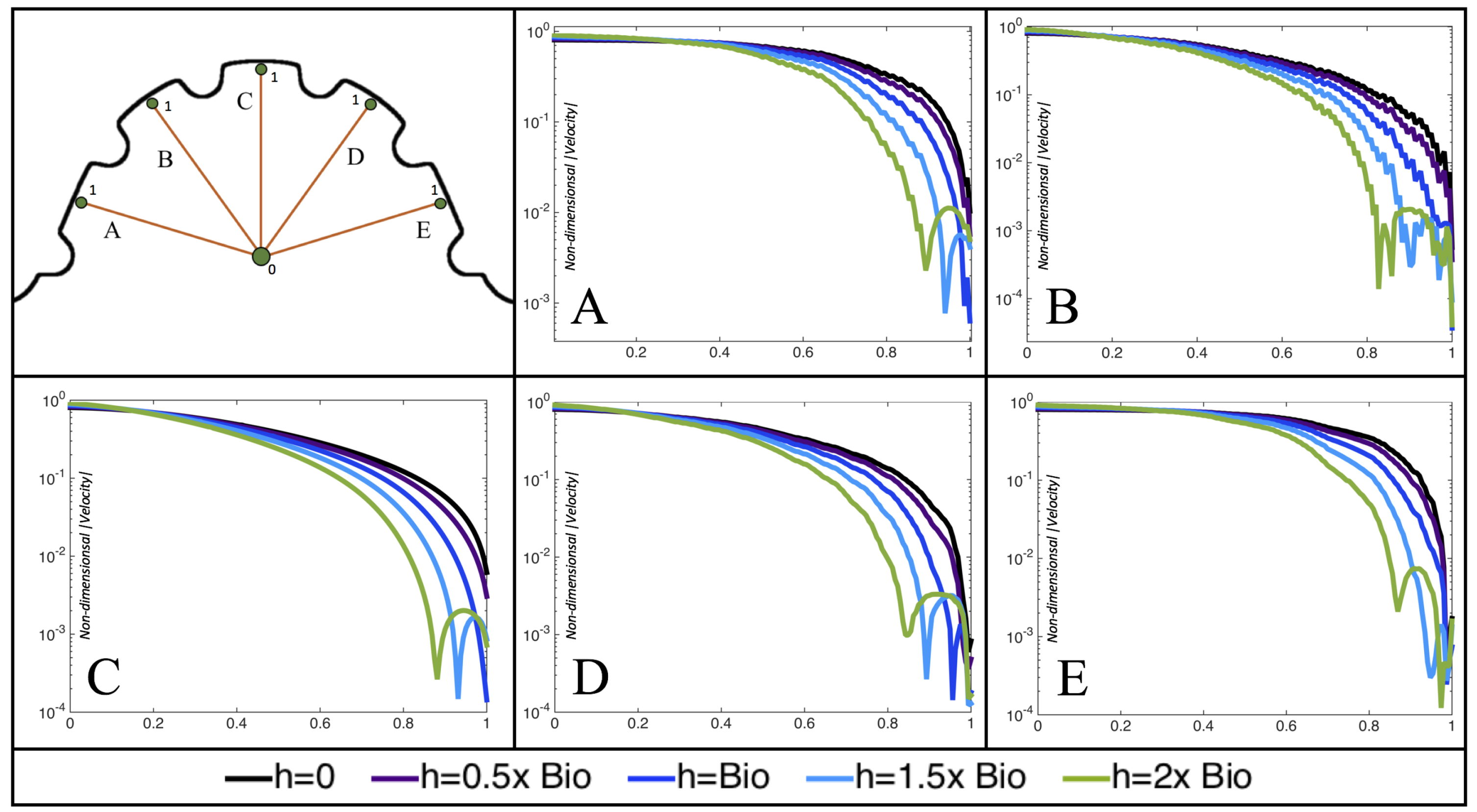
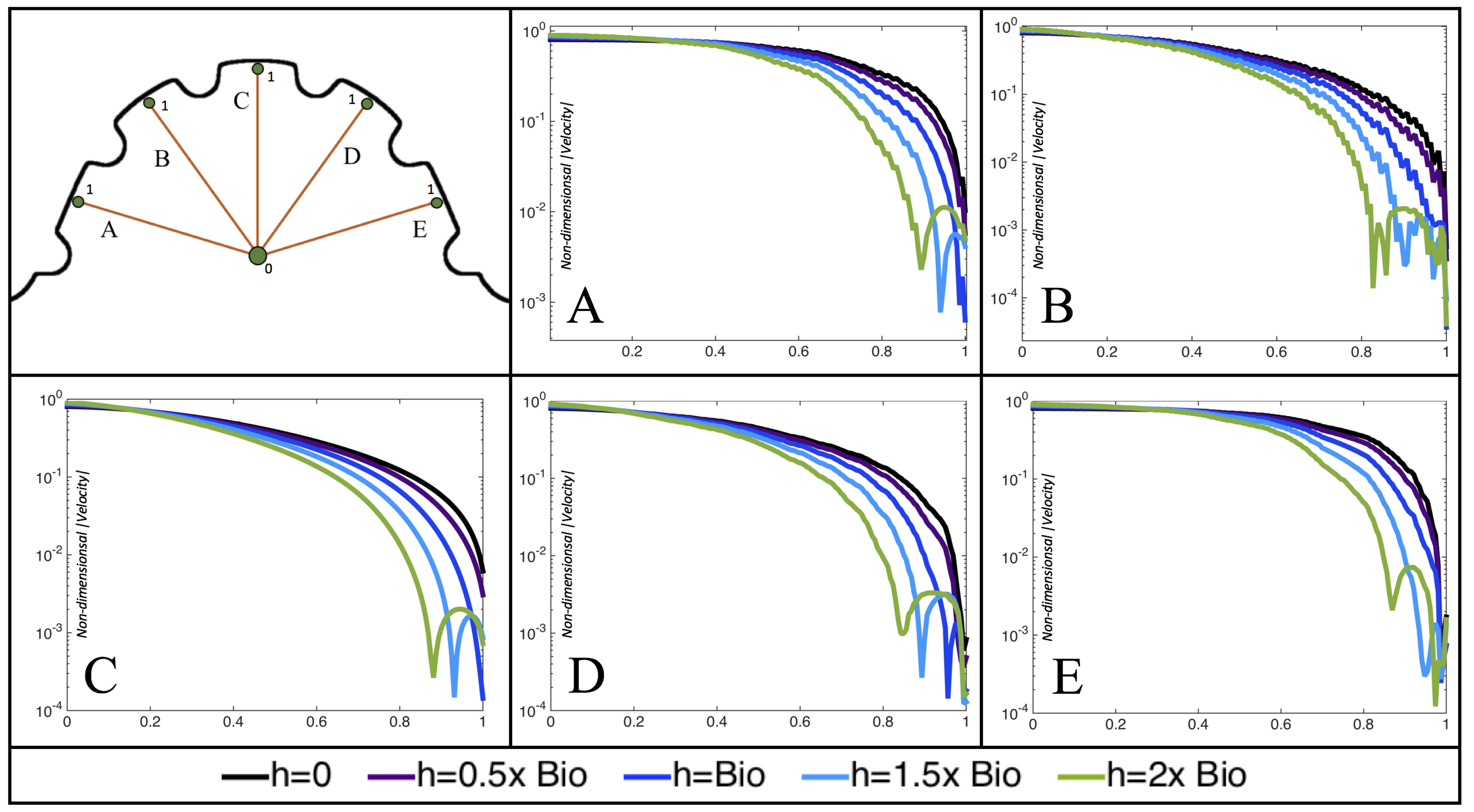
Furthermore, for the biologically relevant case of
,
Figure 17 illustrates the magnitude of velocity from the intracardial center to the ventricular lining for various intertrabecular regions and trabeculae heights. It is clear that, for larger trabeculae heights, the velocity decays moving away from the intracardial center at a faster rate than those cases with shorter or no trabeculae.
When the trabeculae are at biologically relevant heights or larger, the velocity decays from the middle of the ventricle until a distance of that height away from the ventriclular lining. Within that trabecular valley, the velocity actually increases before further decaying when measured closer to the ventricular lining. This shows that a local minima in velocity magnitude exists, suggesting that trabeculae morphology plays an important role in governing the fluid dynamics nearing the ventricular lining. This supports that there is intertrabecular vortex formation in these cases, as shown in
Figure 16. The velocities measured in such intertrabecular regions are less than those shown in the cases with no or smaller trabeculae.
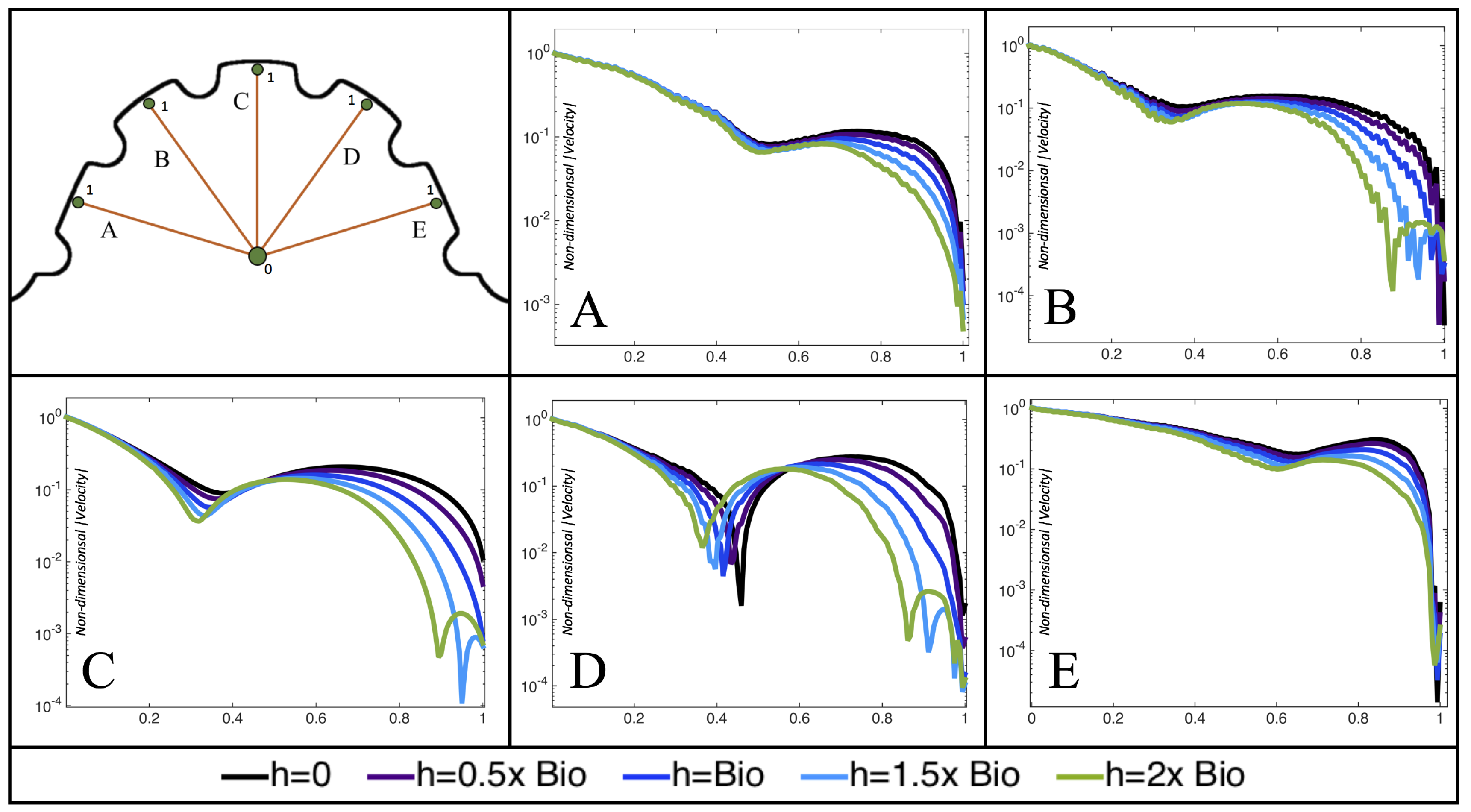
Interestingly, similar results are seen in the
case, see
Figure A6 in
Appendix E. However, in the case of
, slightly different quantitative behavior is observed, see
Figure 18. Note that the local minimum in velocity magnitude is still observed at the neighboring trabeculae height away from the ventricular wall, followed by an increase and then decrease as one moves closer to the wall. In contrast, as you measure away from the intracardial center, the velocity magnitude decreases (as before), but it also increases and then decreases before reaching the trabeculae height distance from the ventricle wall. This is due to the presence of a large intracardial vortex that forms, as illustrated in
Figure 16.
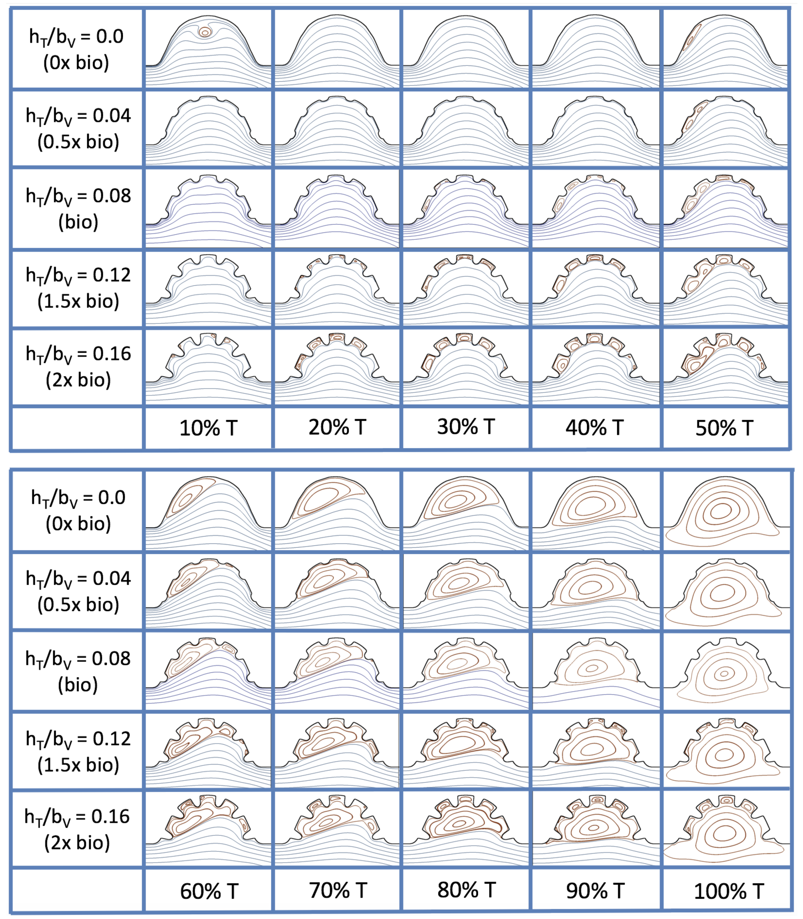
3.4. Pulsatile Flow through Idealized Trabeculated Chambers
Next, we consider the same idealized trabeculated ventricle but use a pulsatile inflow condition, as described in
Appendix A. The pulsation frequency is given by a dimensionless frequency close to that reported for a 4 dpf embryonic zebrafish (
). The
was set to 0.1, 1.0, 10 and 100. The dimensionless trabecular heights,
were varied from 0.0 to 0.16. Recall that the biologically relevant
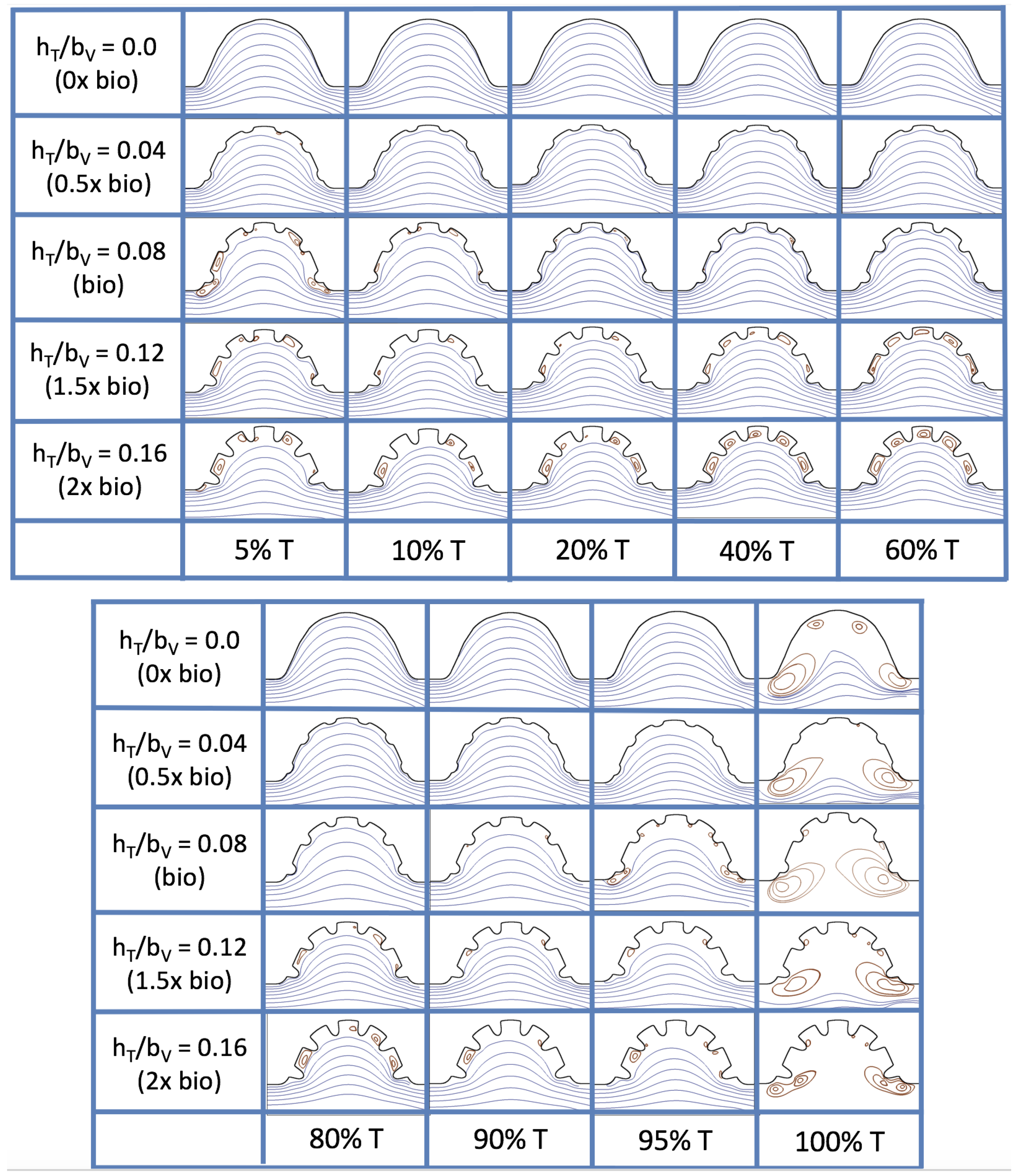
is about one, and the biologically relevant dimensionless trabecular height is about 0.08. Snapshots of the streamlines showing the flow patterns are taken from the last pulse for each simulation using either 9 or 10 time points.
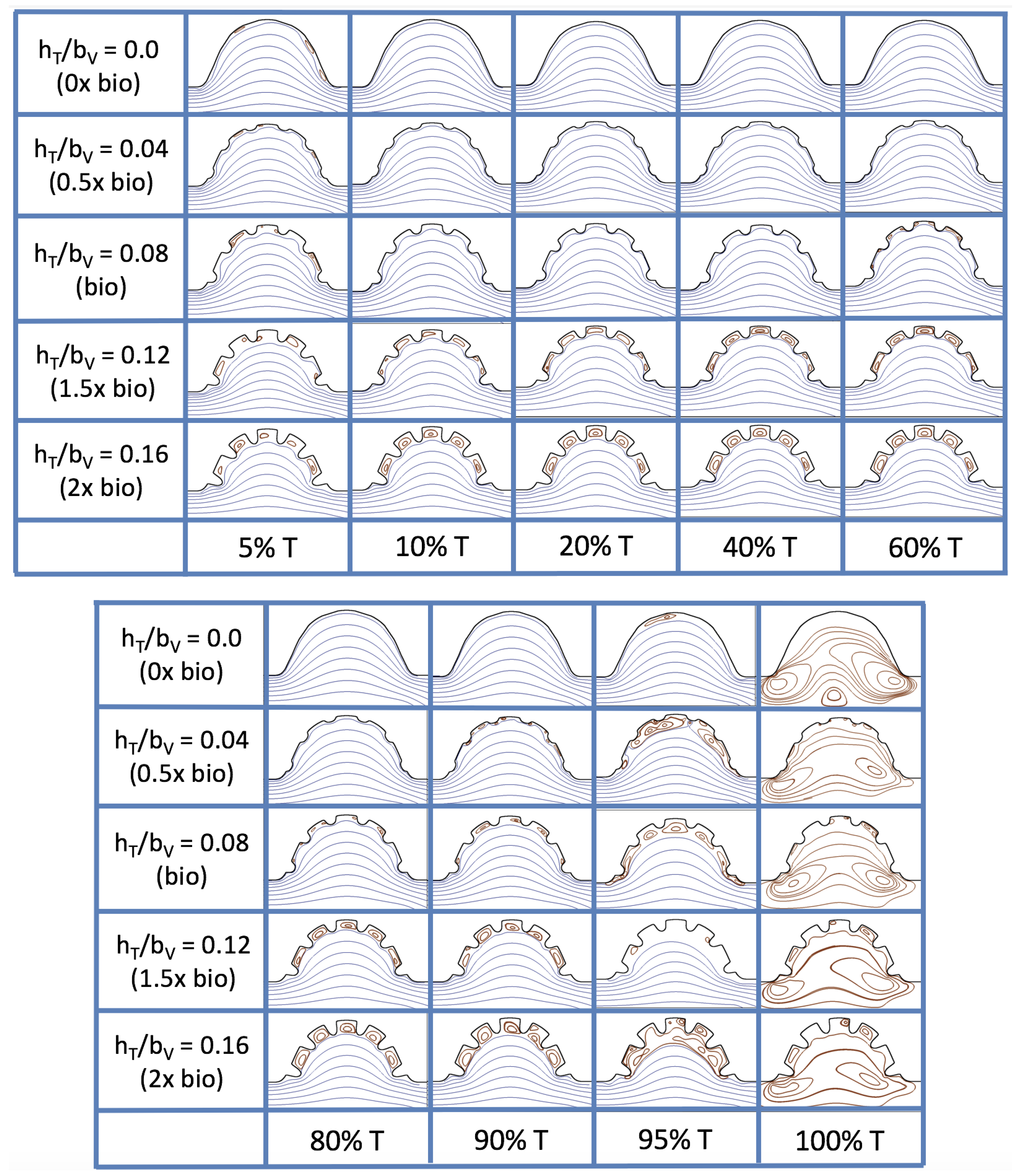
Figure 19 and
Figure 20 show streamline plots taken at nine snapshots in time for lower
cases,
, respectively. The streamlines are shown for 5%, 10%, 20%, 40%, 50%, 80%, 90%, 95%, and 100% of the pulse. Finer increments in time are given towards the beginning and end of the pulse to illustrate the rapidly changing dynamics. The
and
cases show similar results. For the majority of the pulse, the flow moves smoothly from left to right within the ventricle. In between the trabeculae, vortices form during most of the pulse if the dimensionless trabecular height is at least 0.08. The development of these vortices causes the flow near the endothelial cells to move from right to left between the trabeculae and from left to right on the top of the trabeculae. In most cases, transient vortices form as the flow is decelerated at the end of the pulse. For
, intertrabecular vortices form for small trabeculae,
, as the flow decelerates. This is different than in the steady inflow counterpart case in
Section 3.3, where vortex formation only happened for biologically relevant heights or greater.
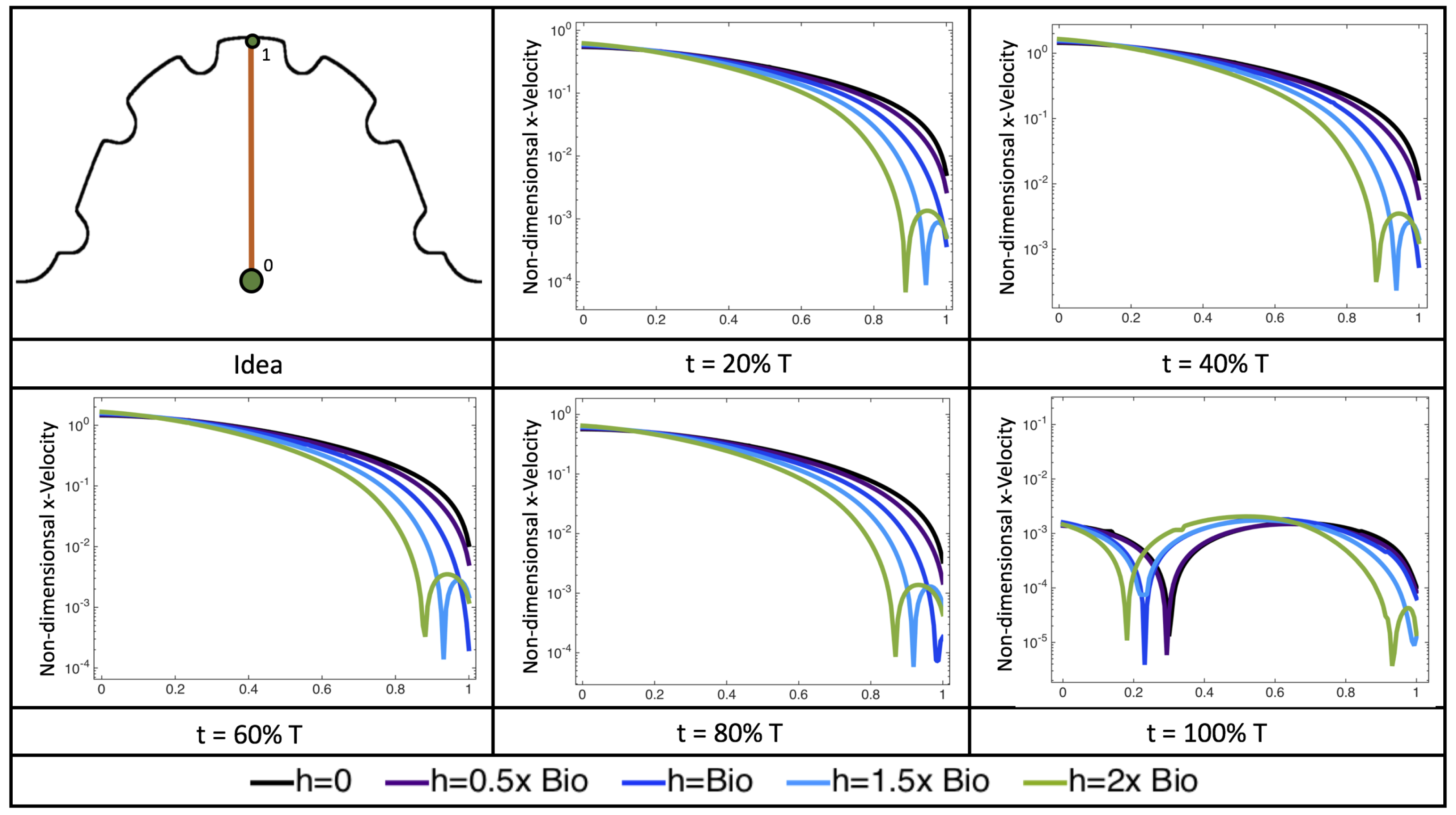
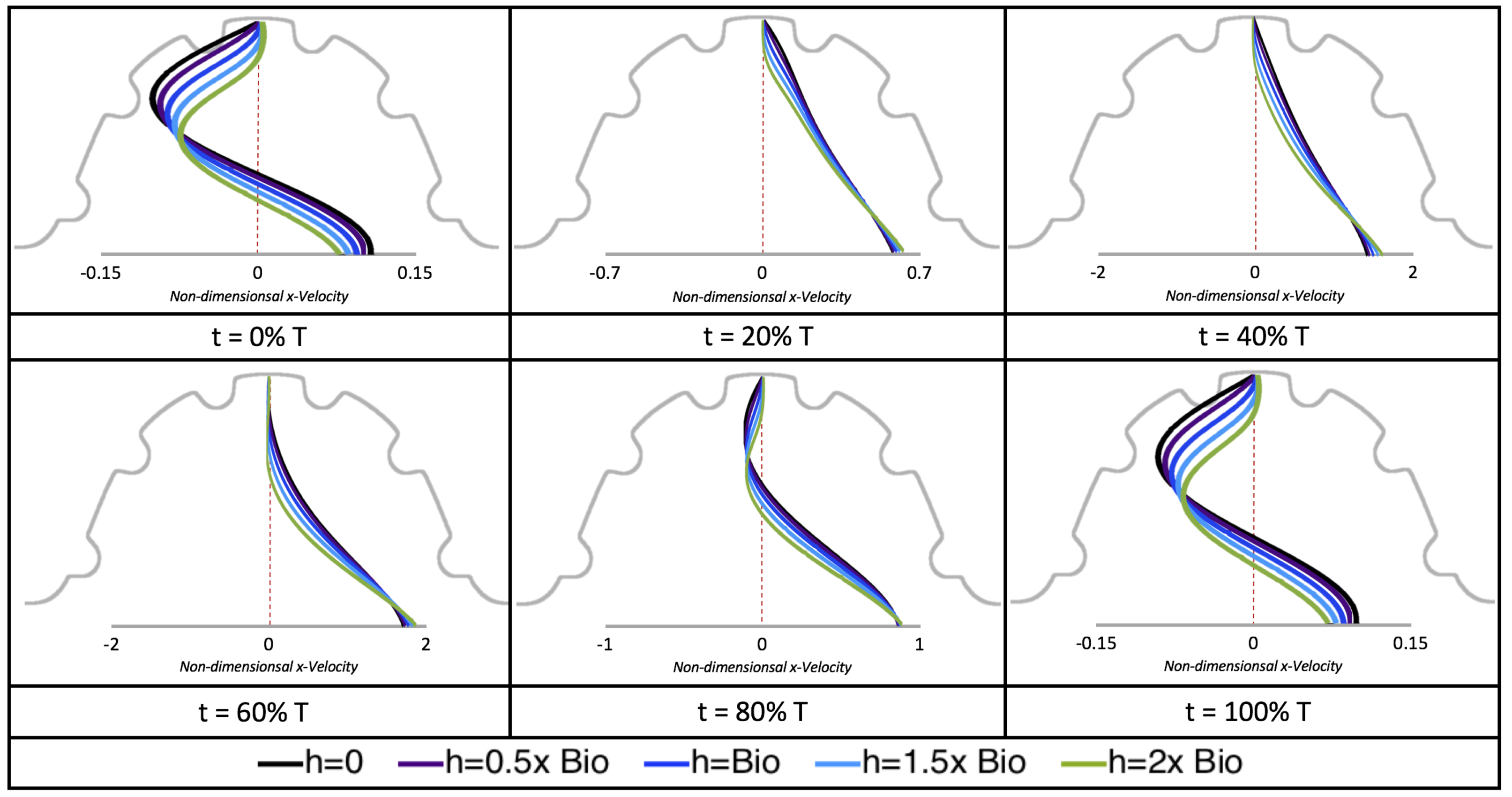
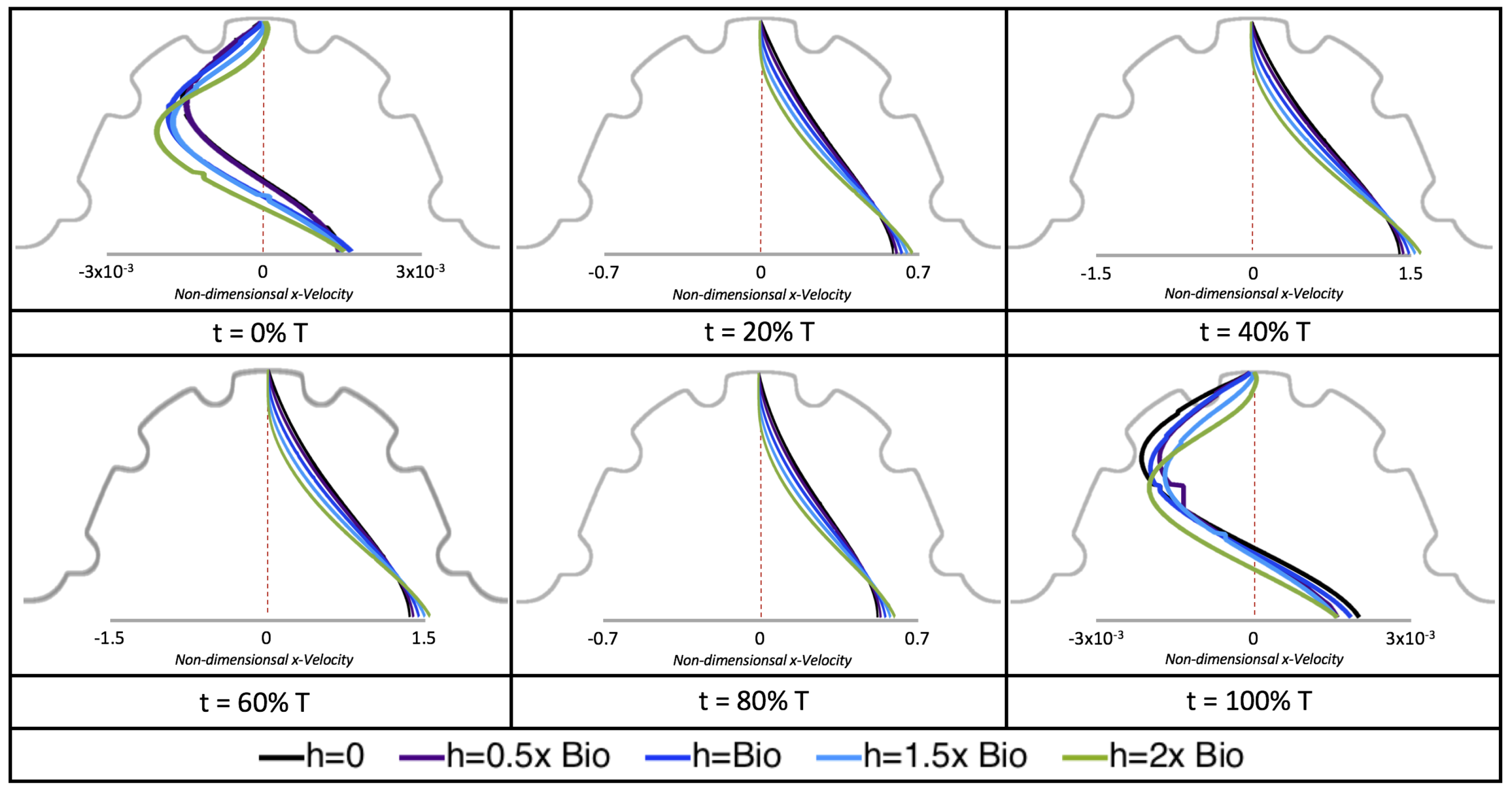
Next, we considered the horizontal velocity extending from the intracardial center to the intertrabecular region directly above it in the case of
. These results are shown in
Figure 21. Flow velocities are at a minimum near the ventricular lining, with the magnitude of velocities decreasing at a slightly accelerated rate for larger trabeculae. On the other hand, at the intracardial center, the horizontal velocity increases with larger trabeculae in the middle of a pulsation cycle. As the pulsation cycle resides, it is clear that the flow direction also changes, giving rise to an intracardial vortex, as detailed in
Figure 20.
Figure 22 shows the magnitude of velocity as as one moves along a line drawn from the top of the ventricle to the base of the middle intratrabecular region for five trabeculae heights five times during the pulse cycle. Note that, during a pulsation cycle, the snapshots taken during the middle of the pulse are similar to that of the steady inflow case for
shown in
Figure 16. For larger trabeculae heights, the horizontal velocity reaches a minimum at distance that is about a trabecular height away from the ventricle wall. As one moves between the trabeculae, the magnitude of the velocity increases and then approaches as one nears the wall. These velocity profiles confirm the formation of vortices as shown in
Figure 20.
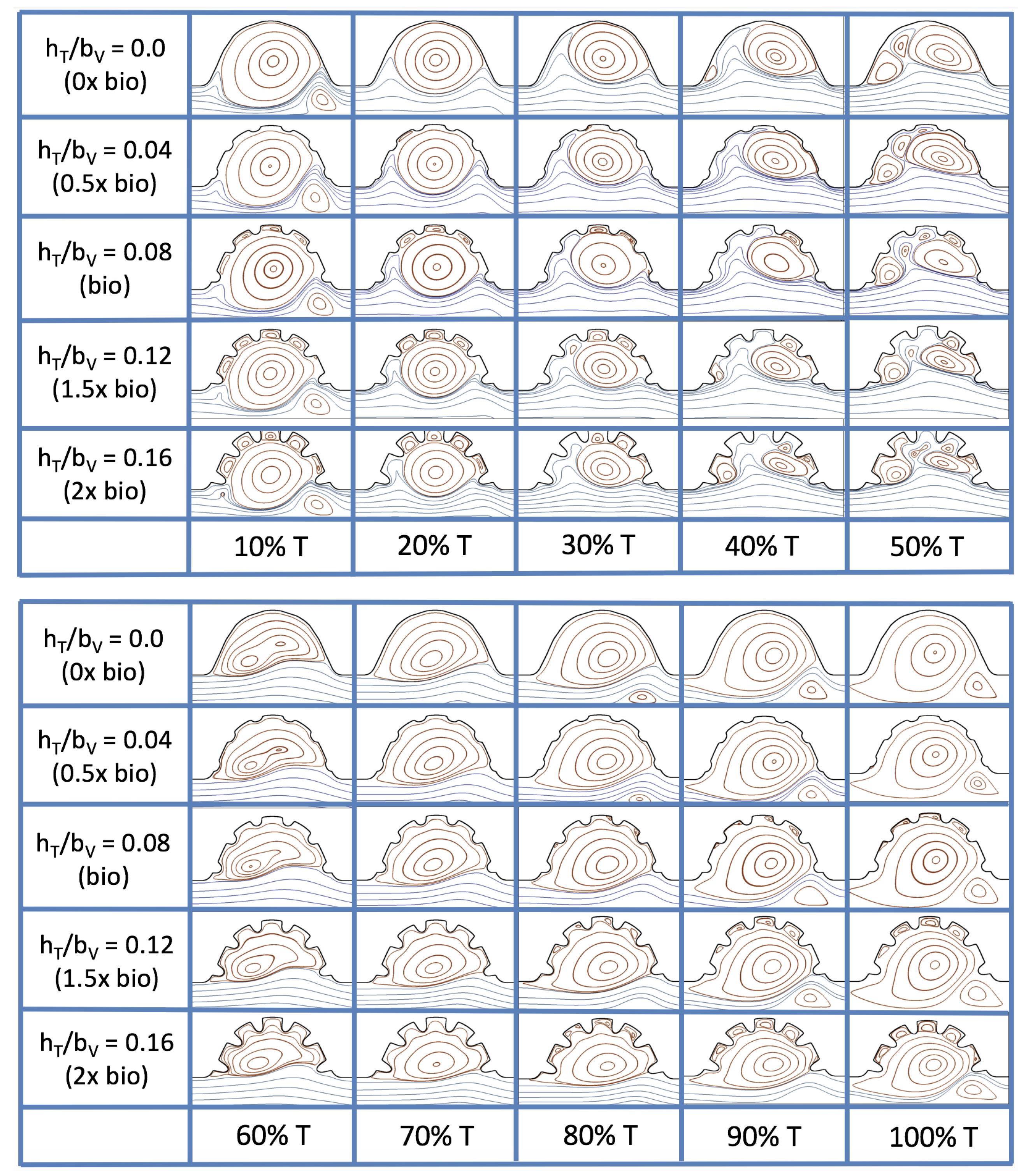
Figure 23 shows streamline plots for
at ten evenly spaced times during a pulse. Intertrabecular vortices form during the first half of the pulse if the dimensionless trabecular height is at least 0.04. For all geometries, intracardial vortices form during the last half of the pulse. The formation of the intracardial vortex annihilates the intertrabecular vortices, at least initially. The intracardial vortices form on the upstream side of the chamber, and grow to fill the entire chamber by the end of the pulse. The intertrabecular vortices form again towards the end of the pulse for
. Note that the presence of the intracardial vortex causes the intertrabecular vortices to change direction so that they spin clockwise (and the intracardial vortices spin counterclockwise).
The spin direction is determined from the laminar flow, given in blue, moving left to right. When vortices first form in the intertrabecular regions, the vortices form moving counterclockwise. However, when a large intracardial vortex forms before intertrabecular vorticies, its direction is counterclockwise, which forces any intertrabecular vortices that form to move clockwise.
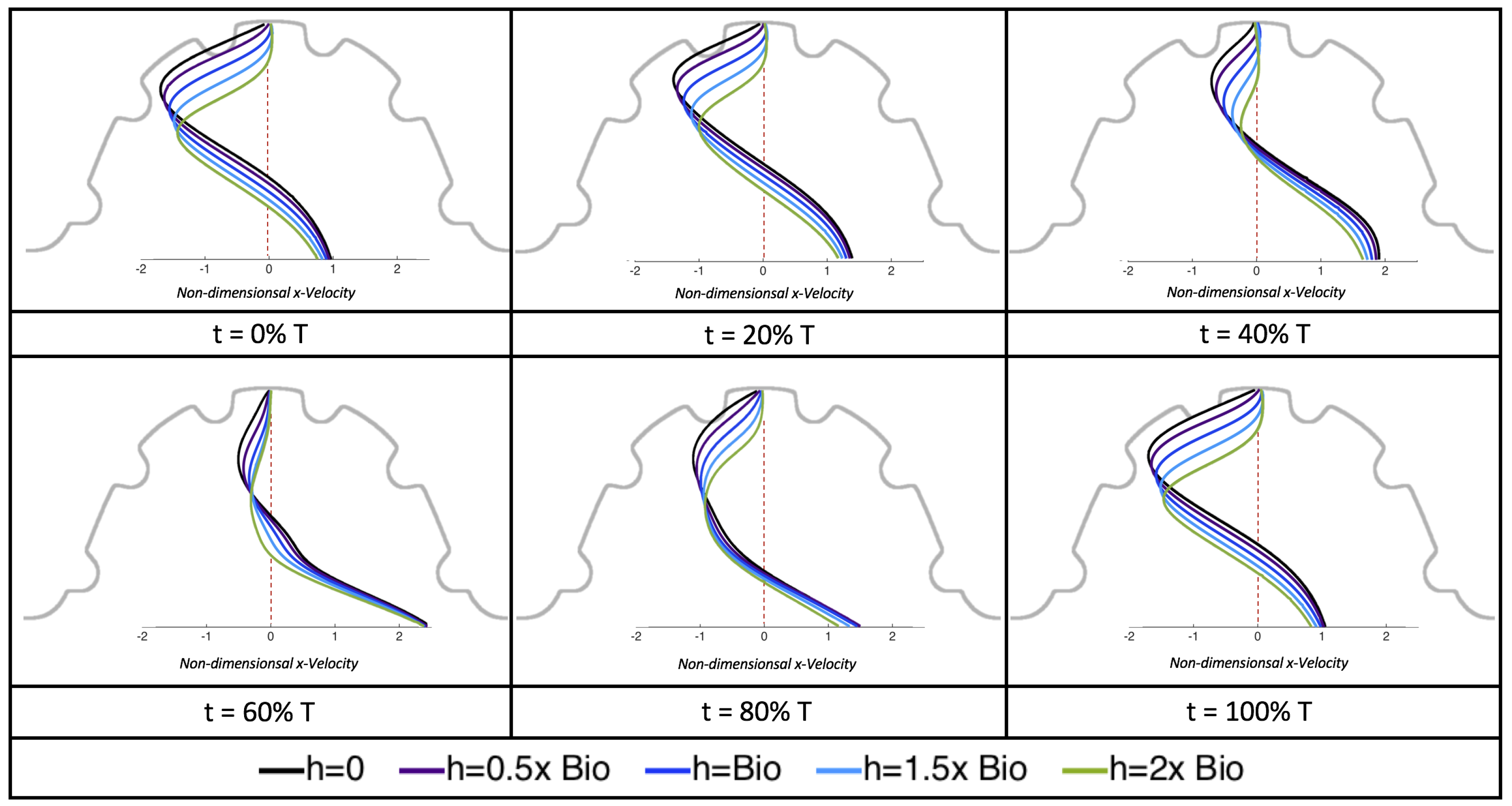
We also considered the horizontal velocity extending from the intracardial center to the intertrabecular region directly above for
, as shown in
Figure 24. Similarly quantitative behavior is seen as in the
case, see
Figure 21; there is still significantly less flow in the intertrabecular region. However, the flow velocities are significantly different in the cavity below the intertrabecular region because of the presence of an intracardial vortex. It is clear that there is flow reversal given the differences in sign of the horizontal velocity.
The results of the inertial dominated case,
, are shown in
Figure 25. In all cases, a large intracardial vortex that fills the entire chamber is observed at the end of the pulse and the beginning of the next pulse. As the flow accelerates, the intracardial vortex is pushed downstream, and another intracardial vortex begins to form (
). One or more oppositely spinning vortices form between the trabeculae or between the two counterclockwise spinning intracardial vortices when
. The upstream intracardial vortex combines with the original intracardial vortex such that one large intracardial vortex is observed around
. When this occurs, the oppositely spinning vortices are annihilated. For
, oppositely spinning intertrabecular vortices reappear at the end of the pulse.
Due to the formation of large intracardial vortices, the horizontal velocity changes sign when measured from the center of the cavity and proceeds directly upward toward the ventricle lining (see
Figure 26). Similar quantitative behavior is seen as in the
case. A substantial difference is the presence of a intracardial vortex that remains largely throughout the pulsation cycle. Moreover, similar to the other cases of
, the velocity is significantly decreased within the intertrabecular region, even for
.
4. Conclusions
Two-dimensional immersed boundary simulations were used to solve for the flow fields within both biologically realistic geometries (3 dpf, 80 hpf, two 5 dpf WT zebrafish and a 7
dpf ErbB2-inhibited zebrafish from [
21]) and idealized models of trabeculated ventricles. Specifically, we investigated the intracardial and intertrabecular fluid dynamics searching for possible vortex formation and spatially-varying velocity gradients.
The primary result of our parametric study using simplified models of the trabeculated embryonic heart is that small changes in morphology and the effective viscosity of the blood can result in significant changes in bulk flow patterns as well as the magnitude and direction of shear felt by the endocardium. This presents an interesting challenge since each of these parameters is continuously changing during development. The results also highlight the importance of obtaining geometric descriptions of the developing heart with high spatial and temporal resolution. Small differences in morphology between individuals may also result in fundamentally different flow signals, underscoring the need to quantify variation. Furthermore, the effective viscosity of the blood is indirectly proportional to
, and small changes in
may also result in drastic changes in flow direction and shear. The effective viscosity of the blood during development likely changes with hematocrit, which also changes from about 10–50% during development, and measurements of embryonic blood rheology are sparse [
5].
This work focused specifically on the presence or absence of vortices given their significance to both the magnitude and direction of flow as well as the mixing patterns within the ventricle. When an intracardial vortex forms, the direction of the flow changes. When an intracardial vortex forms in unsteady flow, the direction of flow can change during the beat cycle, and the stagnation point moves along the cardiac wall. Since endothelial cells are known to sense and respond to changes in both magnitude and direction of flow, the formation and motion of these vortices could be important epigenetic signals.
The simulations revealed unexpected complexities in vortex dynamics as bulk flow moves through the chamber. In the cases of biologically realistic geometries, no large intracardial vortices developed at the biologically realistic fluid scale (
) in the steady inflow case; in the pulsatile case, a large intracardial vortex formed when inflow velocities were minimal between pulses. However, for both steady and pulsatile inflow, intertrabecular vortices formed in pronounced trabeculated regions (
Figure 5 and
Figure 7). While similar behavior was observed in both the steady and pulsatile inflow cases, more vortices formed in the unsteady flow cases in regions with less pronounced trabeculation. These results were consistent with the idealized trabeculation model as well (
Figure 16 and
Figure 20). When vortices form in intertrabecular regions, the flow changes direction in those areas compared to the direction of bulk flow in the chamber. In cases where not all intertrabecular spaces have a vortex, the flow between different trabeculae will move in different directions.
In addition, as expected, the velocity tapers off when measuring flow speeds close to the ventricular lining. In most cases, the flow tapers off approximately three-orders of magnitude before reaching an intertrabecular region. Interestingly, in these regions where there is pronounced vortex formation, the velocity increases and then decreases as it nears the wall (for the pulsatile cases with realistic geometries, see
Figure 10,
Figure 11 and
Figure 12. Note that the corresponding steady inflow cases show similar trends). In the 5 dpf WT (I) case, the velocity may increase an order of magnitude during portions of a pulsation cycle (see
Figure 10), while, in other cases, the increase is modest, such as in the 3 dpf WT case (see
Figure 11). These results are quantitatively similar to those of the idealized model case at
for both pulsatile and steady inflow. The presence of trabeculae appears to control the fluid velocities in this regions, which helps govern the amount of shear-stress felt at the endothelial layer.
It is almost certainly the case that the exact flow patterns and magnitudes will not be exactly the same for realistic geometries with moving walls. Some similar features are observed between our simulations and previous work using idealized geometries with moving walls [
40] as well as realistic geometries with moving walls [
19,
20]. In all cases, there is a severe reduction in flow magnitude in the intratrabecular regions and the presence of intratrabecular vortices exhibiting changes in flow direction and magnitude as a function of intratrabecular depth. The consequences of the reduction in flow magnitude and the presence of vortices are that lower shear stresses are felt at the endothelial wall than would be the case without trabeculae and that the direction of shear changes both spatially and temporally. Direct comparison of our results to work with a moving boundary and idealized geometry [
40] shows that our simplified models do not capture the exact spatial and temporal pattern of flow reversals and shear, but they do demonstrate that these features exist and are sensitive to perturbations in kinematics and morphology.
The idealized model cases expanded the study by allowing us to easily manipulate the system to understand its sensitivity to vortex formation, due to its complex geometry, fluid scale, and inflow characteristics. In this vein, we increased the span of our larger fluid scale from
to
, rather than simply the biological case of
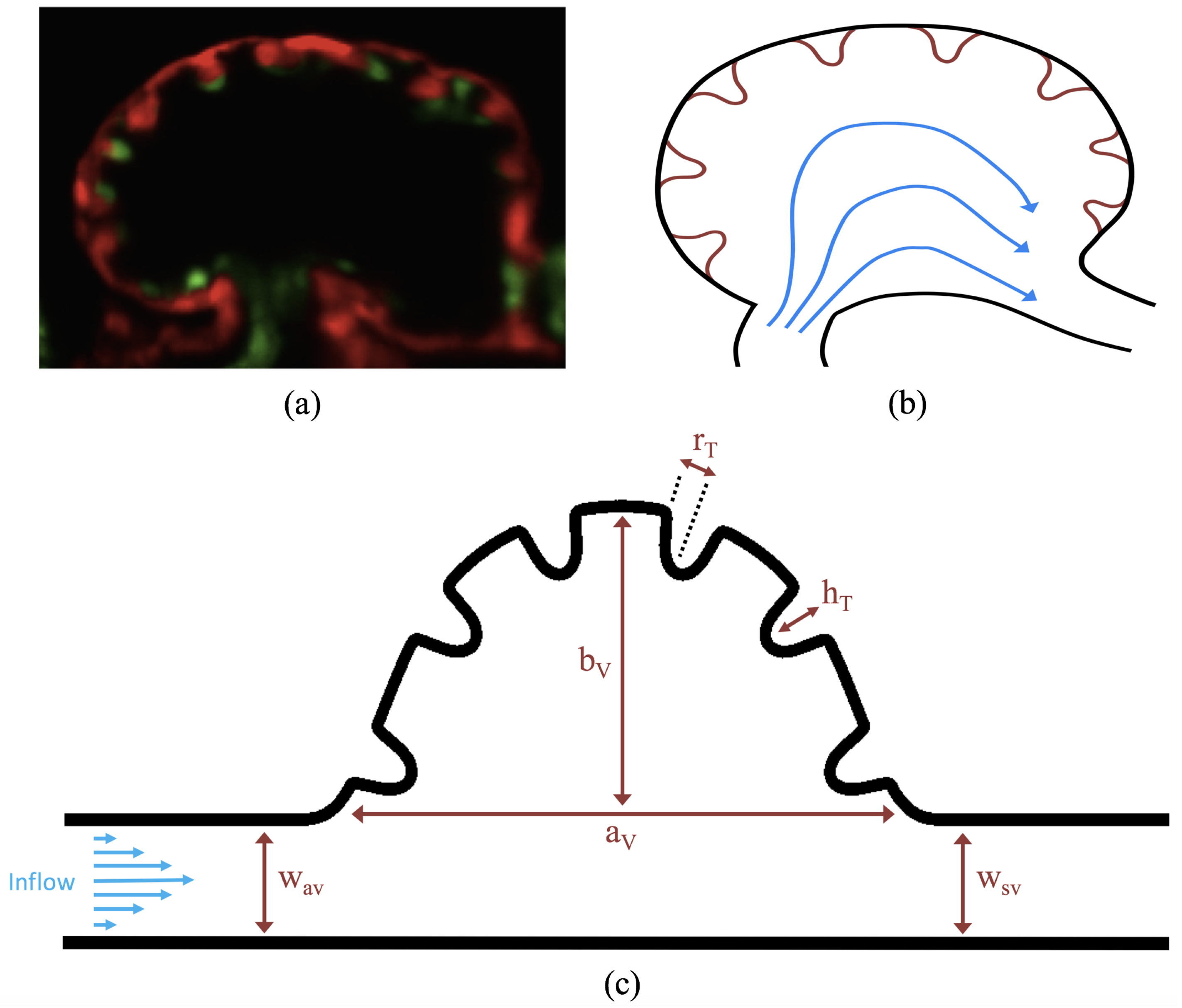
for a 4 dpf embryonic zebrafish heart. We also investigated equally sized idealized trabeculae in a chamber, and varied the heights from no trabeculae to trabeculae twice as large as biologically relevant according to
Figure 3a, and included both pulsatile and steady inflow simulations to parse effects of unsteady flows on vortex formation.
Moreover, diversity of trabeculated hearts across the animal kingdom are far and wide, and may cover a large spectrum of length and fluid (
) scales. Even some invertebrate hearts contain ventricular trabeculation. In those invertebrates, their heart’s morphology resembles that of lower vertebrates with sedentary lifestyles [
50,
51,
52]. Some anthropods and mollusks contain ventiruclar trabeculae, such as blue crabs (
Callinectes sapidus) [
45], bar clams (
Spisula solidissima) [
53], oysters [
54], snails [
55], as well as octopus and squids [
46]. However, any quantitative measurements detailing trabeculae morphology and flow measurements at varying time-points are unknown. It is possible that, in these hearts, the idealized simulations at higher
or for larger trabecular heights are relevant to these invertebrate hearts.
The idealized models showed that a large intracardial vortex forms around
when steady flow is pushed through the chamber, while a similar sized vortex forms for
when the flow is pulsatile. In general, pulsatile flow lowers the
and trabeculae height needed to generate vortices. For both steady and unsteady flows as the trabeculae grow into the chamber, another bifurcation occurs in which small vortices form between each trabecula. Depending upon the
and the morphology, the intertrabecular vortices can form without the presence of a large intracardial vortex (see
Figure 16 for steady cases or
Figure 19 or
Figure 20 for unsteady flow cases of
or
, respectively). In other cases, typically at higher
, both the intracardial and intertrabecular vortices form, see
Figure 23 or
Figure 25, for unsteady inflow for
or 100, respectively. In all corresponding cases, the presence of large intracardial vortices changes the direction of the intertrabecular vortices. Note that, in the biologically relevant case of
intracardial vortices do not form; this is consistent with the biologically accurate geometries as well. We do note that the exact patterns of intracardial and intratrabecular vortex formation may not hold for realistic geometries and pumping kinematics.
It is evident that there is a strongly coupled relationship between intracardial hemodynamics, genetic regulatory networks, and cardiac conduction. Besides contractions of the myocardial cells, which in turn drive blood flow, hemodynamics are directly involved in proper pacemaker and cardiac conduction tissue formation [
56]. In addition, shear stresses are found to govern the conduction velocity distribution of action potentials within the myocardium [
22]. Any changes in the emrbyonic heart’s conduction properties will also affect the intracardial shear stresses, pressures, patterns of cyclic strains, and advection of morphogens. It is indeed a chicken and the egg scenario, especially when considering the first experiments that saw the importance of fluid dynamics in heart morphogenesis were performed in chicken embryos [
57]. Dedicated initiatives to decipher exact cellular signalling pathways and genetic regulatory networks may be able to help further parse the causes of cardiac dysfunction. While CFD provides a robust framework to extract cardiac flow information (fluid velocities, shear stress distributions, pressures, etc.), coupling this data into a multi-scale cellular model is imperative to better understand the causes of many congenital heart diseases.
Unfortunately, the exact mechanisms of mechanotransduction are not yet clearly understood [
58,
59]. Biochemical signals are thought to propagate throughout a pipeline of epigenetic signaling mechanisms, which may regulate of gene expression, cellular differentiation, proliferation, and migration [
60]. In vitro studies have discovered that endothelial cells detect shear stresses as low as 0.2 dyn/cm
, resulting in up or down regulation of gene expressions [
61]. Shear stresses around ∼8–15 dyn/cm
are known to cause cytoskeletal rearrangement [
62]. The aforementioned shear stresses reported in this paper and other CFD studies [
20] are well in the range of those measured within embryonic hearts, ∼2 dyn/cm
and ∼75 dyn/cm
at approximately
and
dpf, respectively [
3]. Mapping out the connection between fluid dynamics, the resulting ventricular stresses, electrophysiology, and the mechanical regulation of developmental regulatory networks are paramount to moving towards a more holistic understanding of heart development.
The simplified models used in this study permitted the exploration of a wide parameter space that includes the diversity of trabeculated hearts in vertebrate embryos and also in some invertebrates. There are obviously limitations in using such simplified models. Flow through the complex trabeculae of the ventricle is inherently three-dimensional. The flows generated by a beating ventricle will be different from pulsatile flows driven through a fixed geometry. Accordingly, our results should motivate the further development of more sophisticated three-dimensional models with complex geometry and moving boundaries. In the development of such models, our results illustrate how critical it is to obtain high resolution geometries and spatially and temporally resolved kinematics. Our results also point towards the consequences of variation in both geometry and blood rheology, which suggest that flow patterns may change drastically through development, between individuals, and across species.

 ,
, 


