
Diagnosis of Epilepsy with Functional Connectivity in EEG after a Suspected First Seizure

 ,
,  ,
,
Abstract
1. Introduction
- Idiopathic: genetically determined epilepsy, usually linked to a particular clinical characteristic;
- Lesional: usually related to a structural abnormality of the brain, an acquired condition;
- Non-lesional: no clear reason is present for the development of brain abnormalities.
- Generalized seizures: originated at some point in the brain, from where a widespread epileptic discharge rapidly involves the entire brain;
- Focal (partial) seizures: originated within networks that are limited to one cerebral hemisphere.
- Functional Segregation: identification of anatomical segregated and specialized cortical regions;
- Functional Integration: identification of interactions among functionally segregated brain regions, analyzing the communication of different brain regions.
2. Methods
2.1. Dataset Description
2.2. EEG Preprocessing
2.3. Epoch Cleaning
2.4. EEG Bipolar Referencing and Scalp Groupings
2.5. Epoch Selection
2.6. Feature Extraction
2.6.1. Band Power Features
2.6.2. Functional Connectivity
- IMCOH: undirected and bivariate measure that is based on the Cartesian representation of the coherency. It has been reported to be quite insensitive to volume conduction artifacts, as well as robust for the identification of te interaction between brain regions, therefore, being a good way of representing brain interactions [37]. IMCOH is defined in Equation (2),where E[] denotes average over epochs, Sxy the cross-spectral density between both EEG signals, Sxx and Syy the power spectral density of the first and second signals, respectively. The latter was computed with the multitaper method [38].
- MI: an information-based measure that evaluates the undirected nonlinear dependence between two signals. MI is bivariate, as well as amplitude-based and time-dependent [11]. It can be computed as Equation (4) suggests,with and representing the probabilities corresponding to signals X and Y, respectively, and the joint probabilities of X and Y.
- PDC: based on autoregressive models (Granger Causality measures). A multivariate autoregressive model (MVAR) models K signals as a linear combination of their own past, plus additional white noise, as Equation (5) shows.X(n) is the signal matrix at time n, E(n) is the matrix containing the uncorrelated white noise at time n, p is the model order and A(m) is the K × K coefficient matrix for delay m. A(m) estimates the influence of sample x(n − m) on the current sample x(n), to which a Fourier transform is applied. PDC is computed with Equation (6).PDC is a measure that is directed, multivariate, linear, amplitude-based and computed in the frequency domain. It is normalized in respect to the outgoing flow, which equals one at each frequency, and it exclusively shows the direct interrelations between the signals [11].
2.6.3. Graph Measures
- In and Out Degrees: these measures are computed only for the PDC, as it is the only directed functional connectivity feature being used. From each scalp group’s matrix, only the maximum values are considered.
- Node strength: after the computation of each channel’s node strength in IMCOH, PLV and MI matrices, the mean and standard deviation values are computed for each scalp group. However, for PDC, only the mean is computed here, as the standard deviation would be strongly correlated with the maximum value of in and out degrees.
- Clustering Coefficient and Betweenness Centrality: just like the node strengths, the mean and standard deviation are calculated from each connectivity matrix for all functional connectivity features.
- Efficiency: the computation of this measure results in one single value for each matrix regarding one subgroup, band and functional connectivity.
2.6.4. Asymmetry Ratios
2.7. Data Split
2.8. Dimensionality Reduction of Feature Space
2.9. Machine Learning Classifier
- Accuracy: measures how often the algorithm classifies a data point correctly, defined in Equation (9),where TP is a true positive, TN a true negative, FP a false positive and FN a false negative;
- Sensitivity: measures the proportion of positives that are correctly identified, also known as true-positive rate (TPR), defined in Equation (10);
- Specificity: measures the proportion of negatives that are correctly identified, also known as false positive rate (FPR), defined in Equation (11);
- Confusion Matrix: a table in which each row represents the instances in an actual class, while each column represents the instances in a predicted class [56];
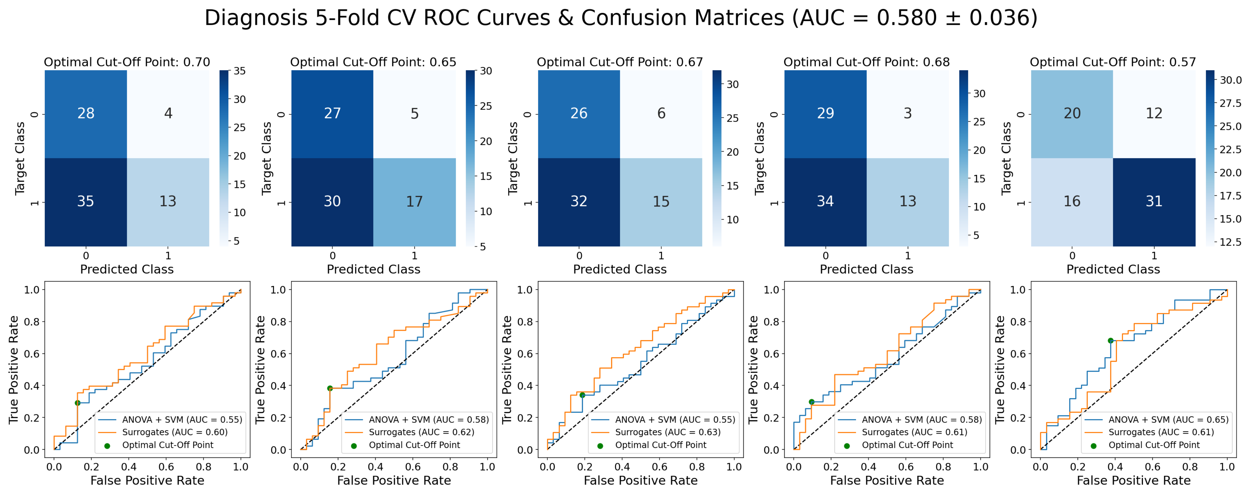
- Receiver Operating Characteristic (ROC) Curve: plots the TPR against the FPR at various threshold settings at which the decision is taken. The optimal cut-off point for a model will be the one that maximizes TPR and minimizes FPR, being used for the computation of the optimal confusion matrix. Surrogate predictions were generated by taking the 95th percentile (for statistical significance) from 100 permuted sets of predictions [57];
- Area under the ROC curve (AUC): it measures the area underneath the ROC curve, ranging from 0 to 1. AUC provides an aggregate measure of performance across all possible classification thresholds [58], being the preferred ML evaluation criterion in this work.
3. Results
3.1. Epileptic vs. Non-Epileptic
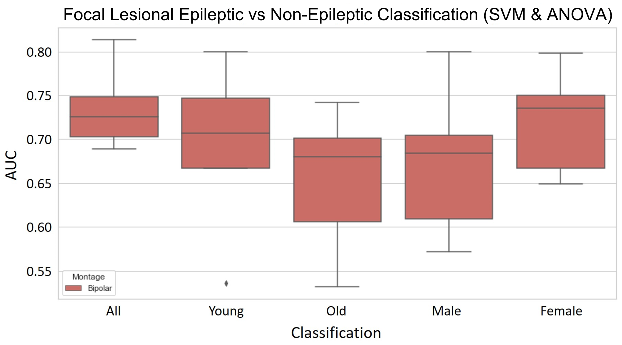
3.2. Focal Lesional Epileptic vs. Non-Epileptic
3.2.1. Validation Results
- The SVM using PCA for dimensionality reduction presents a mean AUC score of 0.730 that, while slightly lower than the same model with ANOVA for feature selection, does present better robustness across the different folds, as shown by the lower standard deviation. The accuracy, sensitivity and specificity are also more balanced and globally higher. As for overfitting, it does not seem to be widely overfit, having a difference in AUC score between the training and validation sets of 0.0255.
- The RFC model shows a mean AUC of 0.745 with a low standard deviation across the five different folds. The values of accuracy, sensitivity and specificity are quite robust too, ranging from 0.699 to 0.730. The major setback of this model is it is overfit to the training set, which presents a difference of 0.254 in the AUC score to the validation set.
- The LogReg using ANOVA and removal of the most correlated features for feature selection presented the best AUC, accuracy and specificity validation scores. It has a mean AUC score of 0.752, with a standard deviation of 0.038. The mean specificity of 0.795 is quite high, even though its standard deviation is considerable. However, the sensitivity is quite poor and the standard deviation shows great dispersion. Overfit-wise, the values of the AUC score between training and validation present a difference of 0.0173, which indicates a low overfit of the training set.
3.2.2. Test Results
3.2.3. Selected Features
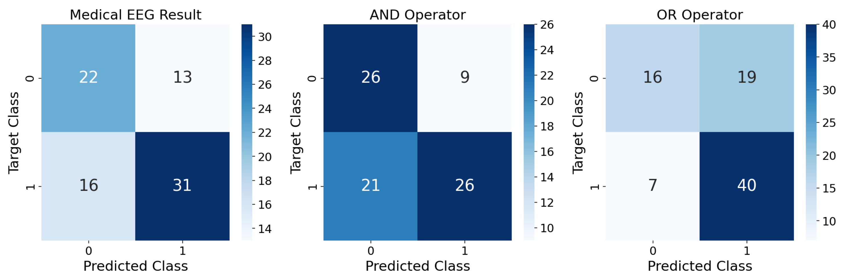
3.3. Performance Comparison against Medical First Evaluation of EEG
4. Discussion
4.1. Focal Lesional Epilepsy-Based Classification
4.2. Performance Comparison against Medical First Evaluation of EEG
4.3. Feature Elimination Based on Correlation
4.4. Future Perspective
5. Conclusions
Author Contributions
Funding
Institutional Review Board Statement
Informed Consent Statement
Data Availability Statement
Conflicts of Interest
Abbreviations
| AL | Anterior-Left |
| AR | Anterior-Right |
| AUC | Area under the receiver operating characteristic curve |
| CT | Computerized Tomography |
| EEG | Electroencephalogram |
| EOG | Electroencephalogram |
| FIR | Finite Impulse Response |
| fMRI | Functional Magnetic Resonance Imaging |
| FN | False Negative |
| FP | False Positive |
| FPR | False Positive Rate |
| GBP | Global Band Power |
| GUH | Geneva University Hospitals |
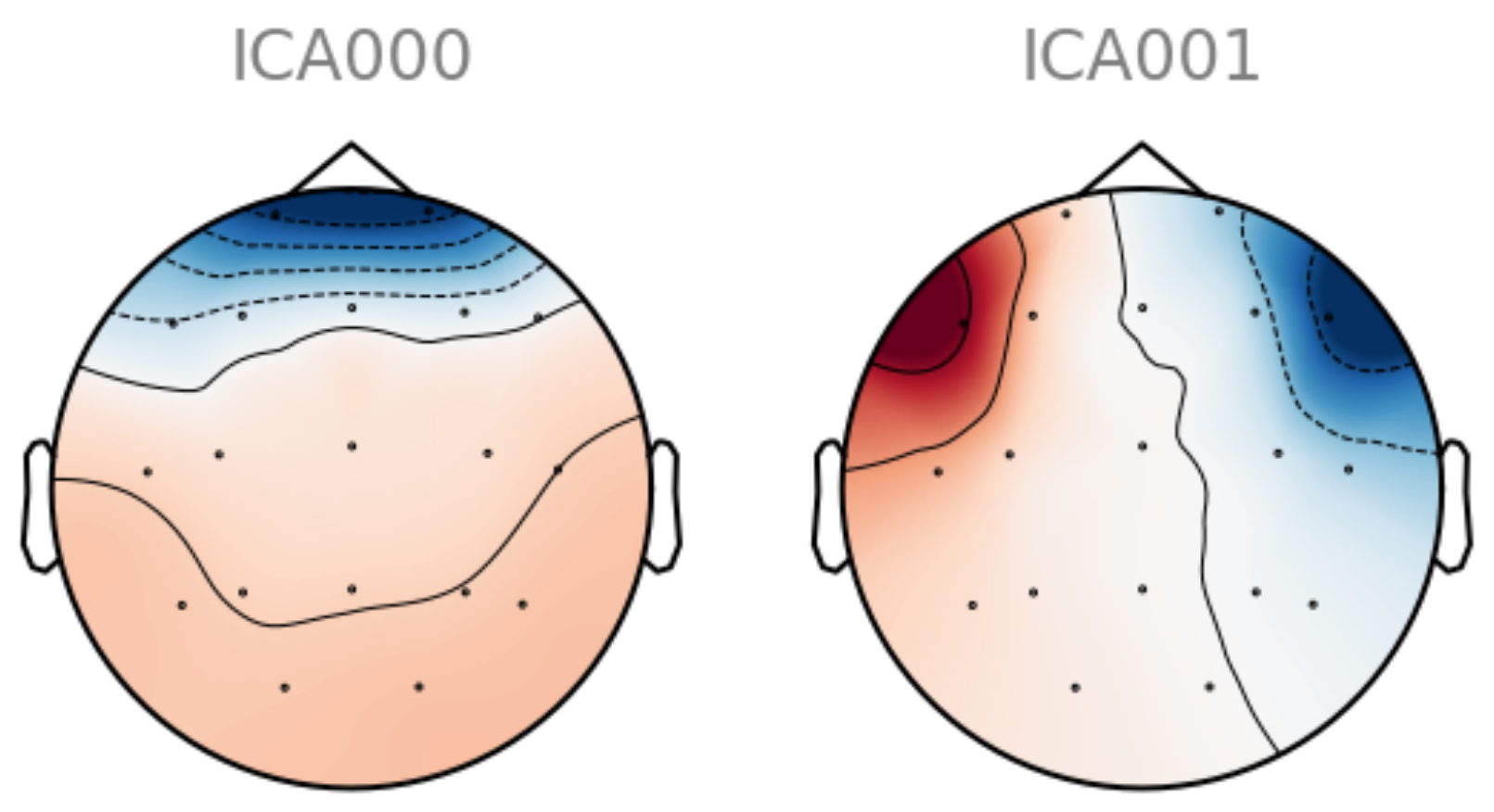
| ICA | Independent Component Analysis |
| IMCOH | Imaginary Part of the Coherency |
| LogReg | Logistic Regression |
| MI | Mutual Information |
| ML | Machine Learning |
| MLP | Multi-layer Perceptron |
| MRI | Magnetic Resonance Imaging |
| MVAR | Multivariate Autoregressive Model |
| PCA | Principal Component Analysis |
| PDC | Partial Directed Coherence |
| PL | Posterior-Left |
| PLV | Phase-Locking Value |
| PR | Posterior-Right |
| RFC | Random Forest Classifier |
| ROC | Receiver Operating Characteristic |
| SVM | Support Vector Machine |
| TN | True Negative |
| TP | True Positive |
| TPR | True Positive Rate |
| WHO | World Health Organization |
Appendix A


References
- Fisher, R.S.; Boas, W.v.E.; Blume, W.; Elger, C.; Genton, P.; Lee, P.; Engel, J., Jr. Epileptic Seizures and Epilepsy: Definitions Proposed by the International League Against Epilepsy (ILAE) and the International Bureau for Epilepsy (IBE). Epilepsia 2005, 46, 470–472. [Google Scholar] [CrossRef] [PubMed]
- Ghaiyoumi, A. Epilepsy Fact Sheet. 2019. Available online: https://epilepsyfoundationmn.org/wp-content/uploads/2019/04/Epilepsy-Fact-Sheet-1.pdf (accessed on 3 February 2021).
- Fisher, R.S.; Acevedo, C.; Arzimanoglou, A.; Bogacz, A.; Cross, J.H.; Elger, C.E.; Engel, J., Jr.; Forsgren, L.; French, J.A.; Glynn, M.; et al. ILAE Official Report: A practical clinical definition of epilepsy. Epilepsia 2014, 55, 475–482. [Google Scholar] [CrossRef] [PubMed]
- Ferrie, C.D. Preventing misdiagnosis of epilepsy. Arch. Dis. Child. 2006, 91, 206–209. [Google Scholar] [CrossRef] [PubMed]
- Krumholz, A.; Wiebe, S.; Gronseth, G.; Shinnar, S.; Levisohn, P.; Ting, T.; Hopp, J.; Shafer, P.; Morris, H.; Seiden, L.; et al. Practice Parameter: Evaluating an apparent unprovoked first seizure in adults (An evidence-based review): [RETIRED]. Neurology 2007, 69, 1996–2007. [Google Scholar] [CrossRef]
- Oto, M.M. The misdiagnosis of epilepsy: Appraising risks and managing uncertainty. Seizure 2017, 44, 143–146. [Google Scholar] [CrossRef]
- WHO. Atlas: Epilepsy Care in the World. 2005. Available online: https://apps.who.int/iris/bitstream/handle/10665/43298/9241563036_eng.pdf?sequence=1&isAllowed=y (accessed on 19 August 2022).
- Roger, J.; Dreifuss, F.; Martinez-Lage, M.; Munari, C.; Porter, R.; Seino, M.; Wolf, P.; Bancaud, J.; Chauvel, P.; Escueta, A.; et al. Proposal for Revised Classification OF Epilepsies and Epileptic Syndromes. Epilepsia 1989, 30, 389–399. [Google Scholar] [CrossRef]
- Engel, J., Jr. Report of the ILAE Classification Core Group. Epilepsia 2006, 47, 1558–1568. [Google Scholar] [CrossRef]
- Panayiotopoulos, C.P. A Clinical Guide to Epileptic Syndromes and Their Treatment; Springer: London, UK, 2010. [Google Scholar] [CrossRef]
- Van Mierlo, P.; Papadopoulou, M.; Carrette, E.; Boon, P.; Vandenberghe, S.; Vonck, K.; Marinazzo, D. Functional brain connectivity from EEG in epilepsy: Seizure prediction and epileptogenic focus localization. Prog. Neurobiol. 2014, 121, 19–35. [Google Scholar] [CrossRef]
- Henry, J.C. Electroencephalography: Basic Principles, Clinical Applications, and Related Fields, Fifth Edition. Neurology 2006, 67, 2092–2092-a. [Google Scholar] [CrossRef]
- Smith, S.J.M. EEG in the diagnosis, classification, and management of patients with epilepsy. J. Neurol. Neurosurg. Psychiatry 2005, 76, ii2–ii7. [Google Scholar] [CrossRef]
- Laufs, H. Functional imaging of seizures and epilepsy: Evolution from zones to networks. Curr. Opin. Neurol. 2012, 25, 194–200. [Google Scholar] [CrossRef]
- Zeki, S.; Shipp, S. The functional logic of cortical connections. Nature 1988, 335, 311–317. [Google Scholar] [CrossRef]
- Mitchell, T.M. Machine Learning; McGraw-Hill: New York, NY, USA, 1997. [Google Scholar]
- Abbasi, B.; Goldenholz, D.M. Machine learning applications in epilepsy. Epilepsia 2019, 60, 2037–2047. [Google Scholar] [CrossRef]
- Coito, A.; Genetti, M.; Pittau, F.; Iannotti, G.; Thomschewski, A.; Höller, Y.; Trinka, E.; Wiest, R.; Seeck, M.; Michel, C.; et al. Altered directed functional connectivity in temporal lobe epilepsy in the absence of interictal spikes: A high density EEG study. Epilepsia 2016, 57, 402–411. [Google Scholar] [CrossRef]
- Carboni, M.; De Stefano, P.; Vorderwülbecke, B.J.; Tourbier, S.; Mullier, E.; Rubega, M.; Momjian, S.; Schaller, K.; Hagmann, P.; Seeck, M.; et al. Abnormal directed connectivity of resting state networks in focal epilepsy. Neuroimage Clin. 2020, 27, 102336. [Google Scholar] [CrossRef]
- Douw, L.; de Groot, M.; van Dellen, E.; Heimans, J.J.; Ronner, H.E.; Stam, C.J.; Reijneveld, J.C. ’Functional connectivity’ is a sensitive predictor of epilepsy diagnosis after the first seizure. PLoS ONE 2010, 5, e10839. [Google Scholar] [CrossRef]
- Van Diessen, E.; Otte, W.M.; Braun, K.P.J.; Stam, C.J.; Jansen, F.E. Improved diagnosis in children with partial epilepsy using a multivariable prediction model based on EEG network characteristics. PLoS ONE 2013, 8, e59764. [Google Scholar] [CrossRef]
- Thomas, J.; Thangavel, P.; Peh, W.Y.; Jing, J.; Yuvaraj, R.; Cash, S.S.; Chaudhari, R.; Karia, S.; Rathakrishnan, R.; Saini, V.; et al. Automated Adult Epilepsy Diagnostic Tool Based on Interictal Scalp Electroencephalogram Characteristics: A Six-Center Study. Int. J. Neural Syst. 2021, 31, 2050074. [Google Scholar] [CrossRef] [PubMed]
- International League Against Epilepsy. ILAE Classification of the Epilepsies (2017). Available online: https://www.ilae.org/guidelines/definition-and-classification/ilae-classification-of-the-epilepsies-2017 (accessed on 19 August 2022).
- Šušmáková, K. Human sleep and sleep EEG. Meas. Sci. Rev. 2004, 4, 59–74. [Google Scholar]
- Gramfort, A.; Luessi, M.; Larson, E.; Engemann, D.A.; Strohmeier, D.; Brodbeck, C.; Goj, R.; Jas, M.; Brooks, T.; Parkkonen, L.; et al. MEG and EEG Data Analysis with MNE-Python. Front. Neurosci. 2013, 7, 1–13. [Google Scholar] [CrossRef] [PubMed]
- Oosugi, N.; Kitajo, K.; Hasegawa, N.; Nagasaka, Y.; Okanoya, K.; Fujii, N. A new method for quantifying the performance of EEG blind source separation algorithms by referencing a simultaneously recorded ECoG signal. Neural Netw. 2017, 93, 1–6. [Google Scholar] [CrossRef]
- Fraschini, M.; Demuru, M.; Crobe, A.; Marrosu, F.; Stam, C.J.; Hillebrand, A. The effect of epoch length on estimated EEG functional connectivity and brain network organisation. J. Neural Eng. 2016, 13, 036015. [Google Scholar] [CrossRef]
- Li, J.; Deng, J.D.; De Ridder, D.; Adhia, D. Gender Classification of EEG Signals using a Motif Attribute Classification Ensemble. In Proceedings of the 2020 International Joint Conference on Neural Networks (IJCNN), Glasgow, UK, 19–24 July 2020; pp. 1–8. [Google Scholar] [CrossRef]
- Jas, M.; Engemann, D.; Raimondo, F.; Bekhti, Y.; Gramfort, A. Automated rejection and repair of bad trials in MEG/EEG. In Proceedings of the 6th International Workshop on Pattern Recognition in Neuroimaging (PRNI), Trento, Italy, 22–24 June 2016. [Google Scholar]
- Wang, S.; Zhang, Y.; Wu, C.; Darvas, F.; Chaovalitwongse, W. Online Prediction of Driver Distraction Based on Brain Activity Patterns. Intell. Transp. Syst. IEEE Trans. 2014, 16, 136–150. [Google Scholar] [CrossRef]
- Vallat, R.; Jajcay, N. raphaelvallat/yasa: v0.4.1. 2021. Available online: https://doi.org/10.5281/zenodo.4632409 (accessed on 19 August 2022). [CrossRef]
- Welch, P. The use of fast Fourier transform for the estimation of power spectra: A method based on time averaging over short, modified periodograms. IEEE Trans. Audio Electroacoust. 1967, 15, 70–73. [Google Scholar] [CrossRef]
- Lundstrom, B.; Boly, M.; Duckrow, R.; Zaveri, H.; Blumenfeld, H. Slowing less than 1 Hz is decreased near the seizure onset zone. Sci. Rep. 2019, 9, 1–10. [Google Scholar] [CrossRef]
- Naftulin, J.S.; Ahmed, O.; Piantoni, G.; Eichenlaub, J.B.; Martinet, L.; Kramer, M.; Cash, S. Ictal and preictal power changes outside of the seizure focus correlate with seizure generalization. Epilepsia 2018, 59, 1398–1409. [Google Scholar] [CrossRef] [PubMed]
- Heers, M.; Helias, M.; Hedrich, T.; Dümpelmann, M.; Schulze-Bonhage, A.; Ball, T. Spectral bandwidth of interictal fast epileptic activity characterizes the seizure onset zone. NeuroImage Clin. 2018, 17, 865–872. [Google Scholar] [CrossRef]
- Li, K.; Guo, L.; Nie, J.; Li, G.; Liu, T. Review of methods for functional brain connectivity detection using fMRI. Comput. Med Imaging Graph. 2009, 33, 131–139. [Google Scholar] [CrossRef]
- Sander, T.; Bock, A.; Leistner, S.; Kühn, A.; Trahms, L. Coherence and imaginary part of coherency identifies cortico-muscular and cortico-thalamic coupling. In Proceedings of the 2010 Annual International Conference of the IEEE Engineering in Medicine and Biology, Buenos Aires, Argentina, 31 August–4 September 2010; pp. 1714–1717. [Google Scholar] [CrossRef]
- Babadi, B.; Brown, E.N. A review of multitaper spectral analysis. IEEE Trans. Biomed. Eng. 2014, 61, 1555–1564. [Google Scholar] [CrossRef] [PubMed]
- Lachaux, J.P.; Rodriguez, E.; Martinerie, J.; Varela, F.J. Measuring phase synchrony in brain signals. Hum. Brain Mapp. 1999, 8, 194–208. [Google Scholar] [CrossRef]
- Nolte, G.; Bai, O.; Wheaton, L.; Mari, Z.; Vorbach, S.; Hallett, M. Identifying true brain interaction from EEG data using the imaginary part of coherency. Clin. Neurophysiol. 2004, 115, 2292–2307. [Google Scholar] [CrossRef] [PubMed]
- Sakkalis, V. Review of advanced techniques for the estimation of brain connectivity measured with EEG/MEG. Comput. Biol. Med. 2011, 41, 1110–1117. [Google Scholar] [CrossRef] [PubMed]
- Baccalá, L.A.; Sameshima, K. Partial directed coherence: A new concept in neural structure determination. Biol. Cybern. 2001, 84, 463–474. [Google Scholar] [CrossRef] [PubMed]
- Pedregosa, F.; Varoquaux, G.; Gramfort, A.; Michel, V.; Thirion, B.; Grisel, O.; Blondel, M.; Prettenhofer, P.; Weiss, R.; Dubourg, V.; et al. Scikit-learn: Machine Learning in Python. J. Mach. Learn. Res. 2011, 12, 2825–2830. [Google Scholar]
- Billinger, M.; Brunner, C.; Müller-Putz, G. SCoT: A Python toolbox for EEG source connectivity. Front. Neuroinform. 2014, 8, 22. [Google Scholar] [CrossRef]
- Rubinov, M.; Sporns, O. Complex network measures of brain connectivity: Uses and interpretations. NeuroImage 2010, 52, 1059–1069. [Google Scholar] [CrossRef]
- Achard, S.; Bullmore, E. Efficiency and Cost of Economical Brain Functional Networks. PLoS Comput. Biol. 2007, 3, e17. [Google Scholar] [CrossRef]
- Orchard, E.R.; Ward, P.G.D.; Chopra, S.; Storey, E.; Egan, G.F.; Jamadar, S.D. Neuroprotective Effects of Motherhood on Brain Function in Late Life: A Resting-State fMRI Study. Cereb. Cortex 2020, 31, 1270–1283. [Google Scholar] [CrossRef]
- Lee, Y.Y.; Hsieh, S. Classifying Different Emotional States by Means of EEG-Based Functional Connectivity Patterns. PLoS ONE 2014, 9, e95415. [Google Scholar] [CrossRef]
- Murphy, K. Machine Learning: A Probabilistic Perspective; Adaptive Computation and Machine Learning Series; MIT Press: Cambridge, MA, USA, 2012. [Google Scholar]
- Cortes, C.; Vapnik, V. Support-Vector Networks. Mach. Learn. 1995, 20, 273–297. [Google Scholar] [CrossRef]
- Baum, E.B. On the capabilities of multilayer perceptrons. J. Complex. 1988, 4, 193–215. [Google Scholar] [CrossRef]
- Riedmiller, M. Advanced supervised learning in multi-layer perceptrons—From backpropagation to adaptive learning algorithms. Comput. Stand. Interfaces 1994, 16, 265–278. [Google Scholar] [CrossRef]
- Loh, W.Y. Classification and regression trees. WIREs Data Min. Knowl. Discov. 2011, 1, 14–23. [Google Scholar] [CrossRef]
- Breiman, L. Random Forests. Mach. Learn. 2001, 45, 5–32. [Google Scholar] [CrossRef]
- Dreiseitl, S.; Ohno-Machado, L. Logistic regression and artificial neural network classification models: A methodology review. J. Biomed. Inform. 2002, 35, 352–359. [Google Scholar] [CrossRef]
- Powers, D. Evaluation: From Precision, Recall and F-Factor to ROC, Informedness, Markedness & Correlation. Mach. Learn. Technol. 2008, 2, 37–63. [Google Scholar]
- Proix, T.; Truccolo, W.; Leguia, M.G.; Tcheng, T.K.; King-Stephens, D.; Rao, V.R.; Baud, M.O. Forecasting seizure risk in adults with focal epilepsy: A development and validation study. Lancet. Neurol. 2021, 20, 127–135. [Google Scholar] [CrossRef]
- Fawcett, T. An introduction to ROC analysis. Pattern Recognit. Lett. 2006, 27, 861–874. [Google Scholar] [CrossRef]
- Gilmore, P.C.; Brenner, R.P. Correlation of EEG, computerized tomography, and clinical findings: Study of 100 patients with focal delta activity. Arch. Neurol. 1981, 38, 371–372. [Google Scholar] [CrossRef]
- Marshall, D.W.; Brey, R.L.; Morse, M.W. Focal and/or lateralized polymorphic delta activity: Association with either ‘normal’ or ‘nonfocal’ computed tomographic scans. Arch. Neurol. 1988, 45, 33–35. [Google Scholar] [CrossRef]
- Quraan, M.A.; McCormick, C.; Cohn, M.; Valiante, T.A.; McAndrews, M.P. Altered Resting State Brain Dynamics in Temporal Lobe Epilepsy Can Be Observed in Spectral Power, Functional Connectivity and Graph Theory Metrics. PLoS ONE 2013, 8, 1–14. [Google Scholar] [CrossRef] [PubMed]
- Rasheed, K.; Qayyum, A.; Qadir, J.; Sivathamboo, S.; Kawn, P.; Kuhlmann, L.; O’Brien, T.; Razi, A. Machine Learning for Predicting Epileptic Seizures Using EEG Signals: A Review. IEEE Rev. Biomed. Eng. 2020, 14, 139–155. [Google Scholar] [CrossRef] [PubMed]


| Type of Feature | Feature | Comments |
|---|---|---|
| Band Power | Delta (1–4 Hz) Theta (4–8 Hz) Alpha (8–13 Hz) Beta (13–30 Hz) Total Absolute Power (1–30 Hz) | Epochs combined with median and std. Scalp groupings: AL, AR, PL, PR. |
| Functional Connectivity | Imaginary Part of Coherency (IMCOH) Phase-Locking Value (PLV) Mutual Information (MI) Partial Directed Coherence (PDC) | Epochs combined with mean, except for MI, which combines epochs with median, and PDC that combines epochs in MVAR. Five different frequency bands. Scalp groupings: AL, AR, PL, PR, spatially combined with mean and standard deviation. |
| Graph Measure | Efficiency Betweenness Centrality Clustering Coefficient Node Strength In and Out Degrees (directed, PDC only) | Epochs combined with mean, except for MI, which combines epochs with median, and PDC that combines epochs in MVAR. Five different frequency bands. Scalp groupings: AL, AR, PL, PR, spatially combined with mean and standard deviation. |
| Asymmetry Ratios | Anterior: left vs. right (AL vs. AR) Posterior: left vs. right (PL vs. PR) | Based on graph measures, which summarize connectivity matrices. Ratios only relative to mean values from Betweeness Centrality, Clustering Coefficient and Node Strengths; maximum value from In and Out degrees. |
| # | Model | AUC | Accuracy | Sensitivity | Specificity | Val vs. Train |
|---|---|---|---|---|---|---|
| 1 | SVM (linear) and ANOVA | 0.736 ± 0.044 | 0.689 ± 0.052 | 0.856 ± 0.031 | 0.531 ± 0.102 | 0.0426 |
| 2 | SVM (gaussian) and PCA | 0.730 ± 0.030 | 0.705 ± 0.020 | 0.692 ± 0.084 | 0.717 ± 0.061 | 0.0255 |
| 3 | SVM (linear) and Corr-ANOVA | 0.735 ± 0.037 | 0.689 ± 0.034 | 0.672 ± 0.162 | 0.704 ± 0.118 | 0.0345 |
| 4 | MLP and ANOVA | 0.732 ± 0.047 | 0.717 ± 0.051 | 0.749 ± 0.116 | 0.688 ± 0.117 | 0.0082 |
| 5 | MLP and PCA | 0.734 ± 0.026 | 0.698 ± 0.018 | 0.674 ± 0.141 | 0.724 ± 0.141 | 0.0576 |
| 6 | RFC | 0.745 ± 0.022 | 0.714 ± 0.012 | 0.730 ± 0.069 | 0.699 ± 0.048 | 0.254 |
| 7 | RFC and ANOVA | 0.718 ± 0.047 | 0.686 ± 0.050 | 0.767 ± 0.080 | 0.609 ± 0.161 | 0.282 |
| 8 | RFC and PCA | 0.706 ± 0.022 | 0.698 ± 0.023 | 0.655 ± 0.117 | 0.742 ± 0.140 | 0.272 |
| 9 | LogReg and ANOVA | 0.734 ± 0.048 | 0.698 ± 0.057 | 0.775 ± 0.209 | 0.629 ± 0.205 | 0.0344 |
| 10 | LogReg and PCA | 0.729 ± 0.033 | 0.698 ± 0.023 | 0.704 ± 0.107 | 0.693 ± 0.131 | 0.0028 |
| 11 | LogReg and Corr-ANOVA | 0.752 ± 0.038 | 0.717 ± 0.037 | 0.634 ± 0.189 | 0.795 ± 0.153 | 0.0173 |
| Final Model | AUC | Accuracy | Sensitivity | Specificity |
|---|---|---|---|---|
| SVM and PCA | 0.649 | 0.671 | 0.745 | 0.571 |
| RFC | 0.655 | 0.646 | 0.723 | 0.543 |
| LogReg Corr-ANOVA | 0.624 | 0.598 | 0.574 | 0.629 |
Publisher’s Note: MDPI stays neutral with regard to jurisdictional claims in published maps and institutional affiliations. |
© 2022 by the authors. Licensee MDPI, Basel, Switzerland. This article is an open access article distributed under the terms and conditions of the Creative Commons Attribution (CC BY) license (https://creativecommons.org/licenses/by/4.0/).
Share and Cite
Matos, J.; Peralta, G.; Heyse, J.; Menetre, E.; Seeck, M.; van Mierlo, P. Diagnosis of Epilepsy with Functional Connectivity in EEG after a Suspected First Seizure. Bioengineering 2022, 9, 690. https://doi.org/10.3390/bioengineering9110690
Matos J, Peralta G, Heyse J, Menetre E, Seeck M, van Mierlo P. Diagnosis of Epilepsy with Functional Connectivity in EEG after a Suspected First Seizure. Bioengineering. 2022; 9(11):690. https://doi.org/10.3390/bioengineering9110690
Chicago/Turabian StyleMatos, João, Guilherme Peralta, Jolan Heyse, Eric Menetre, Margitta Seeck, and Pieter van Mierlo. 2022. "Diagnosis of Epilepsy with Functional Connectivity in EEG after a Suspected First Seizure" Bioengineering 9, no. 11: 690. https://doi.org/10.3390/bioengineering9110690
APA StyleMatos, J., Peralta, G., Heyse, J., Menetre, E., Seeck, M., & van Mierlo, P. (2022). Diagnosis of Epilepsy with Functional Connectivity in EEG after a Suspected First Seizure. Bioengineering, 9(11), 690. https://doi.org/10.3390/bioengineering9110690