
Cross-Subject Motor Imagery Electroencephalogram Decoding with Domain Generalization

Abstract
1. Introduction
2. Methods
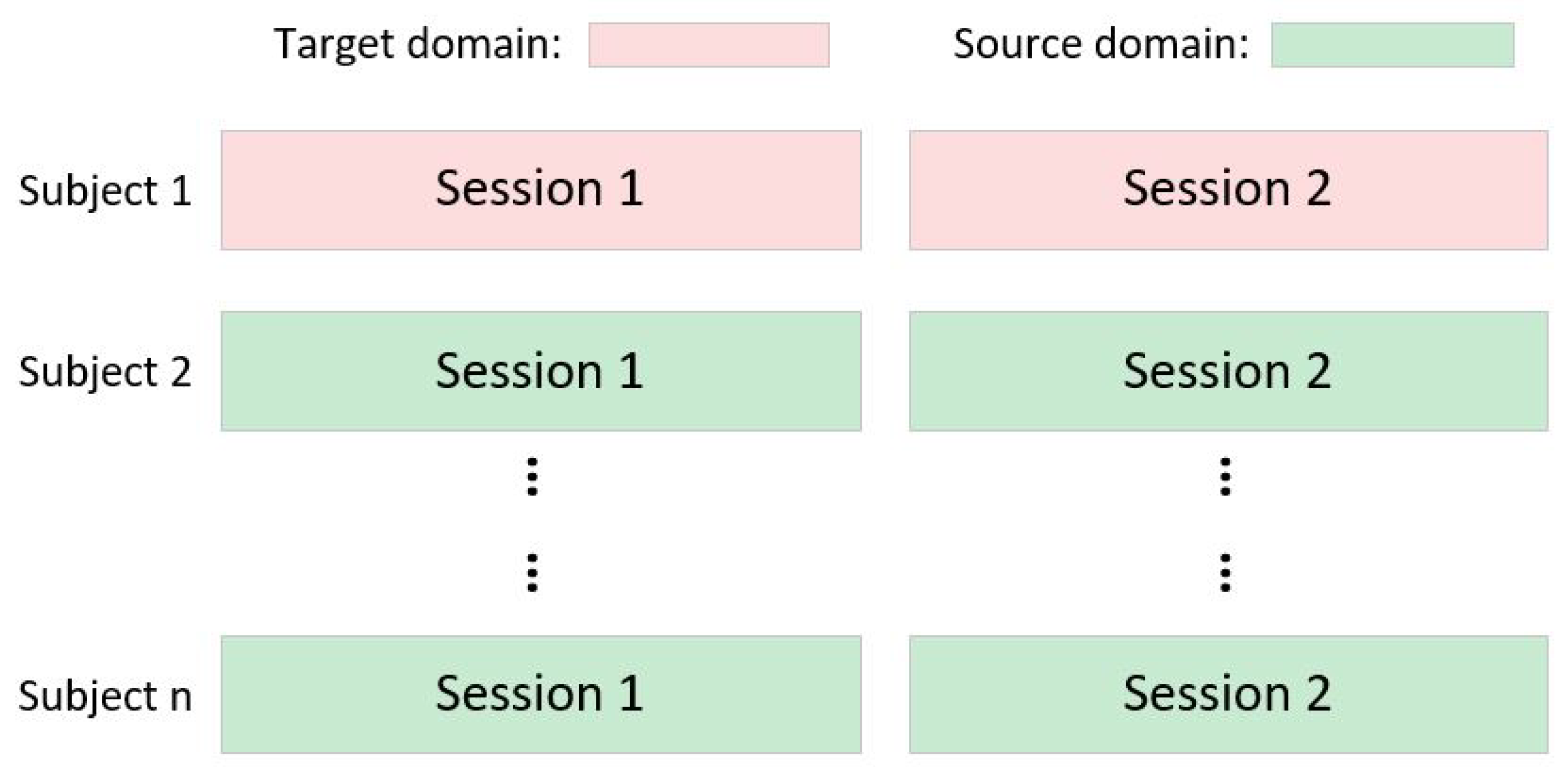
2.1. Definitions
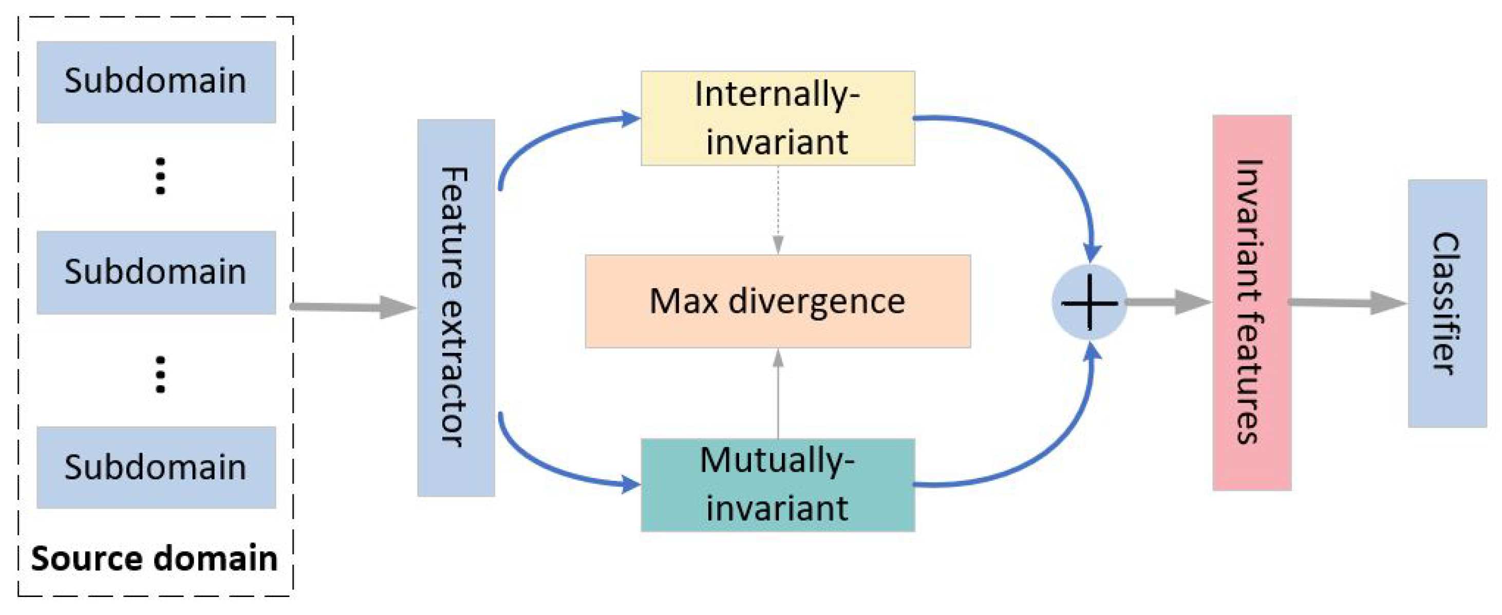
2.2. Framework
2.3. Internally Invariant Features
2.3.1. Spectral Feature Fusion
2.3.2. Feature Extractor
2.3.3. Classifier
2.4. Mutually Invariant Features
3. Experiments and Results
3.1. Datasets
3.1.1. Dataset I
3.1.2. Dataset II
3.2. Training Procedure
3.3. Baseline Models
3.3.1. Machine Learning Approaches
3.3.2. CNN-Based Approaches
3.3.3. Dynamic CNN-Based Approaches
3.4. Experimental Results
3.5. Ablation Study
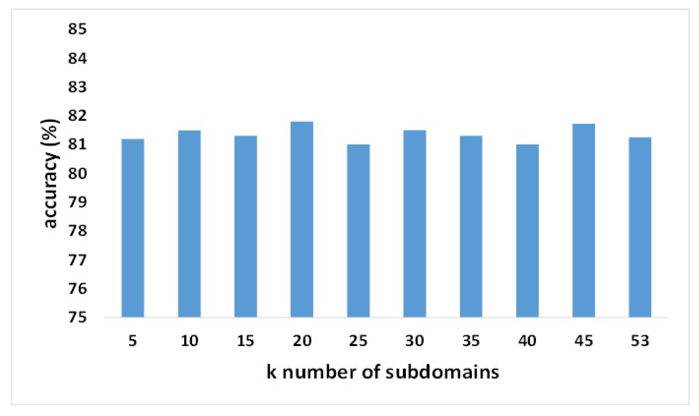
3.6. Parameter Sensitivity
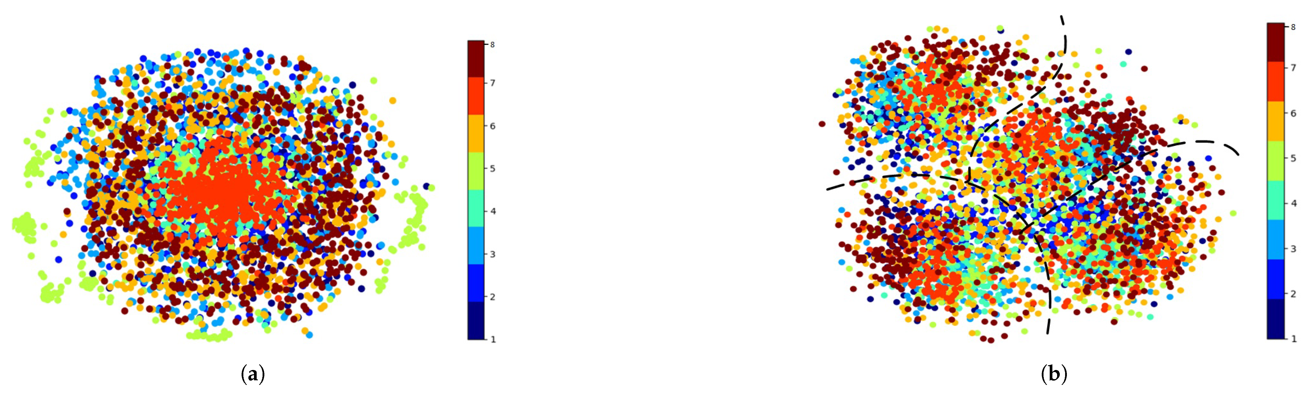
3.7. Visualization
3.8. Limitations
4. Discussion
5. Conclusions
Author Contributions
Funding
Data Availability Statement
Acknowledgments
Conflicts of Interest
References
- Teplan, M. Fundamentals of EEG measurement. Meas. Sci. Rev. 2002, 2, 1–11. [Google Scholar]
- Buzsáki, G.; Anastassiou, C.A.; Koch, C. The origin of extracellular fields and currents—EEG, ECoG, LFP and spikes. Nat. Rev. Neurosci. 2012, 13, 407–420. [Google Scholar] [CrossRef]
- Abdelhameed, A.M.; Bayoumi, M. Semi-supervised deep learning system for epileptic seizures onset prediction. In Proceedings of the 2018 17th IEEE International Conference on Machine Learning and Applications (ICMLA), Orlando, FL, USA, 17–20 December 2018; pp. 1186–1191. [Google Scholar]
- Jeong, J. EEG dynamics in patients with Alzheimer’s disease. Clin. Neurophysiol. 2004, 115, 1490–1505. [Google Scholar] [CrossRef]
- Sánchez-Reyes, L.M.; Rodríguez-Reséndiz, J.; Avecilla-Ramírez, G.N.; García-Gomar, M.L.; Robles-Ocampo, J.B. Impact of eeg parameters detecting dementia diseases: A systematic review. IEEE Access 2021, 9, 78060–78074. [Google Scholar] [CrossRef]
- Chowdhury, P.; Shakim, S.K.; Karim, M.R.; Rhaman, M.K. Cognitive efficiency in robot control by Emotiv EPOC. In Proceedings of the 2014 International Conference on Informatics, Electronics & Vision (ICIEV), Dhaka, Bangladesh, 23–24 May 2014; pp. 1–6. [Google Scholar]
- Grude, S.; Freeland, M.; Yang, C.; Ma, H. Controlling mobile Spykee robot using Emotiv neuro headset. In Proceedings of the 32nd Chinese Control Conference, Xi’an, China, 26–28 July 2013; pp. 5927–5932. [Google Scholar]
- Shao, L.; Zhang, L.; Belkacem, A.N.; Zhang, Y.; Chen, X.; Li, J.; Liu, H. EEG-controlled wall-crawling cleaning robot using SSVEP-based brain-computer interface. J. Healthc. Eng. 2020, 2020, 6968713. [Google Scholar] [CrossRef]
- Suhaimi, N.S.; Mountstephens, J.; Teo, J. EEG-based emotion recognition: A state-of-the-art review of current trends and opportunities. Comput. Intell. Neurosci. 2020, 2020, 8875426. [Google Scholar] [CrossRef]
- Mane, R.; Chew, E.; Phua, K.S.; Ang, K.K.; Robinson, N.; Vinod, A.; Guan, C. Prognostic and monitory EEG-biomarkers for BCI upper-limb stroke rehabilitation. IEEE Trans. Neural Syst. Rehabil. Eng. 2019, 27, 1654–1664. [Google Scholar] [CrossRef] [PubMed]
- Mane, R.; Chouhan, T.; Guan, C. BCI for stroke rehabilitation: Motor and beyond. J. Neural Eng. 2020, 17, 041001. [Google Scholar] [CrossRef] [PubMed]
- Al-Qazzaz, N.K.; Alyasseri, Z.A.A.; Abdulkareem, K.H.; Ali, N.S.; Al-Mhiqani, M.N.; Guger, C. EEG feature fusion for motor imagery: A new robust framework towards stroke patients rehabilitation. Comput. Biol. Med. 2021, 137, 104799. [Google Scholar] [CrossRef]
- Craik, A.; He, Y.; Contreras-Vidal, J.L. Deep learning for electroencephalogram (EEG) classification tasks: A review. J. Neural Eng. 2019, 16, 031001. [Google Scholar] [CrossRef]
- Pfurtscheller, G.; Neuper, C. Motor imagery and direct brain-computer communication. Proc. IEEE 2001, 89, 1123–1134. [Google Scholar] [CrossRef]
- Lemm, S.; Blankertz, B.; Curio, G.; Muller, K.R. Spatio-spectral filters for improving the classification of single trial EEG. IEEE Trans. Biomed. Eng. 2005, 52, 1541–1548. [Google Scholar] [CrossRef] [PubMed]
- Novi, Q.; Guan, C.; Dat, T.H.; Xue, P. Sub-band common spatial pattern (SBCSP) for brain-computer interface. In Proceedings of the 2007 3rd International IEEE/EMBS Conference on Neural Engineering, Kohala Coast, HI, USA, 2–5 May 2007; pp. 204–207. [Google Scholar]
- Ang, K.K.; Chin, Z.Y.; Zhang, H.; Guan, C. Filter bank common spatial pattern (FBCSP) in brain-computer interface. In Proceedings of the 2008 IEEE International Joint Conference on Neural Networks (IEEE World Congress on Computational Intelligence), Hong Kong, China, 1–8 June 2008; pp. 2390–2397. [Google Scholar]
- Subasi, A.; Gursoy, M.I. EEG signal classification using PCA, ICA, LDA and support vector machines. Expert Syst. Appl. 2010, 37, 8659–8666. [Google Scholar] [CrossRef]
- Schirrmeister, R.T.; Springenberg, J.T.; Fiederer, L.D.J.; Glasstetter, M.; Eggensperger, K.; Tangermann, M.; Hutter, F.; Burgard, W.; Ball, T. Deep learning with convolutional neural networks for EEG decoding and visualization. Hum. Brain Mapp. 2017, 38, 5391–5420. [Google Scholar] [CrossRef]
- Lawhern, V.J.; Solon, A.J.; Waytowich, N.R.; Gordon, S.M.; Hung, C.P.; Lance, B.J. EEGNet: A compact convolutional neural network for EEG-based brain–computer interfaces. J. Neural Eng. 2018, 15, 056013. [Google Scholar] [CrossRef] [PubMed]
- Mane, R.; Robinson, N.; Vinod, A.P.; Lee, S.W.; Guan, C. A multi-view CNN with novel variance layer for motor imagery brain computer interface. In Proceedings of the 2020 42nd Annual International Conference of the IEEE Engineering in Medicine & Biology Society (EMBC), Montreal, QC, Canada, 20–24 July 2020; pp. 2950–2953. [Google Scholar]
- Li, Y.; Guo, L.; Liu, Y.; Liu, J.; Meng, F. A temporal-spectral-based squeeze-and-excitation feature fusion network for motor imagery EEG decoding. IEEE Trans. Neural Syst. Rehabil. Eng. 2021, 29, 1534–1545. [Google Scholar] [CrossRef]
- Song, Y.; Zheng, Q.; Liu, B.; Gao, X. EEG Conformer: Convolutional Transformer for EEG Decoding and Visualization. IEEE Trans. Neural Syst. Rehabil. Eng. 2022, 31, 710–719. [Google Scholar] [CrossRef]
- Vaswani, A.; Shazeer, N.; Parmar, N.; Uszkoreit, J.; Jones, L.; Gomez, A.N.; Kaiser, Ł.; Polosukhin, I. Attention is all you need. Adv. Neural Inf. Process. Syst. 2017, 30. [Google Scholar]
- Roy, Y.; Banville, H.; Albuquerque, I.; Gramfort, A.; Falk, T.H.; Faubert, J. Deep learning-based electroencephalography analysis: A systematic review. J. Neural Eng. 2019, 16, 051001. [Google Scholar] [CrossRef]
- Wang, M.; Deng, W. Deep visual domain adaptation: A survey. Neurocomputing 2018, 312, 135–153. [Google Scholar] [CrossRef]
- Chen, Y.; Hang, W.; Liang, S.; Liu, X.; Li, G.; Wang, Q.; Qin, J.; Choi, K.S. A novel transfer support matrix machine for motor imagery-based brain computer interface. Front. Neurosci. 2020, 14, 606949. [Google Scholar] [CrossRef] [PubMed]
- Wei, F.; Xu, X.; Jia, T.; Zhang, D.; Wu, X. A Multi-Source Transfer Joint Matching Method for Inter-Subject Motor Imagery Decoding. IEEE Trans. Neural Syst. Rehabil. Eng. 2023, 31, 1258–1267. [Google Scholar] [CrossRef] [PubMed]
- Liang, Y.; Ma, Y. Calibrating EEG features in motor imagery classification tasks with a small amount of current data using multisource fusion transfer learning. Biomed. Signal Process. Control 2020, 62, 102101. [Google Scholar] [CrossRef]
- Zhuang, F.; Qi, Z.; Duan, K.; Xi, D.; Zhu, Y.; Zhu, H.; Xiong, H.; He, Q. A comprehensive survey on transfer learning. Proc. IEEE 2020, 109, 43–76. [Google Scholar] [CrossRef]
- Hang, W.; Feng, W.; Du, R.; Liang, S.; Chen, Y.; Wang, Q.; Liu, X. Cross-subject EEG signal recognition using deep domain adaptation network. IEEE Access 2019, 7, 128273–128282. [Google Scholar] [CrossRef]
- Chen, P.; Gao, Z.; Yin, M.; Wu, J.; Ma, K.; Grebogi, C. Multiattention adaptation network for motor imagery recognition. IEEE Trans. Syst. Man Cybern. Syst. 2021, 52, 5127–5139. [Google Scholar] [CrossRef]
- Hong, X.; Zheng, Q.; Liu, L.; Chen, P.; Ma, K.; Gao, Z.; Zheng, Y. Dynamic joint domain adaptation network for motor imagery classification. IEEE Trans. Neural Syst. Rehabil. Eng. 2021, 29, 556–565. [Google Scholar] [CrossRef] [PubMed]
- Dose, H.; Møller, J.S.; Iversen, H.K.; Puthusserypady, S. An end-to-end deep learning approach to MI-EEG signal classification for BCIs. Expert Syst. Appl. 2018, 114, 532–542. [Google Scholar] [CrossRef]
- Zhang, K.; Robinson, N.; Lee, S.W.; Guan, C. Adaptive transfer learning for EEG motor imagery classification with deep convolutional neural network. Neural Netw. 2021, 136, 1–10. [Google Scholar] [CrossRef]
- Tobin, J.; Fong, R.; Ray, A.; Schneider, J.; Zaremba, W.; Abbeel, P. Domain randomization for transferring deep neural networks from simulation to the real world. In Proceedings of the 2017 IEEE/RSJ International Conference on Intelligent Robots and Systems (IROS), Vancouver, BC, Canada, 24–28 September 2017; pp. 23–30. [Google Scholar]
- Zhang, H.; Cisse, M.; Dauphin, Y.N.; Lopez-Paz, D. mixup: Beyond empirical risk minimization. arXiv 2017, arXiv:1710.09412. [Google Scholar]
- Wang, J.; Lan, C.; Liu, C.; Ouyang, Y.; Qin, T.; Lu, W.; Chen, Y.; Zeng, W.; Yu, P.S. Generalizing to Unseen Domains: A Survey on Domain Generalization. IEEE Trans. Knowl. Data Eng. 2023, 35, 8052–8072. [Google Scholar] [CrossRef]
- Grubinger, T.; Birlutiu, A.; Schöner, H.; Natschläger, T.; Heskes, T. Domain generalization based on transfer component analysis. In Proceedings of the Advances in Computational Intelligence: 13th International Work-Conference on Artificial Neural Networks, IWANN 2015, Palma de Mallorca, Spain, 10–12 June 2015; pp. 325–334. [Google Scholar]
- Pan, S.J.; Tsang, I.W.; Kwok, J.T.; Yang, Q. Domain adaptation via transfer component analysis. IEEE Trans. Neural Netw. 2010, 22, 199–210. [Google Scholar] [CrossRef] [PubMed]
- Muandet, K.; Balduzzi, D.; Schölkopf, B. Domain Generalization via Invariant Feature Representation. In Proceedings of the 30th International Conference on Machine Learning, Atlanta, GA, USA, 17–19 June 2013; Dasgupta, S., McAllester, D., Eds.; Proceedings of Machine Learning Research. Volume 28, pp. 10–18. [Google Scholar]
- Ghifary, M.; Balduzzi, D.; Kleijn, W.B.; Zhang, M. Scatter Component Analysis: A Unified Framework for Domain Adaptation and Domain Generalization. IEEE Trans. Pattern Anal. Mach. Intell. 2017, 39, 1414–1430. [Google Scholar] [CrossRef] [PubMed]
- Li, Y.; Tian, X.; Gong, M.; Liu, Y.; Liu, T.; Zhang, K.; Tao, D. Deep Domain Generalization via Conditional Invariant Adversarial Networks. In Proceedings of the European Conference on Computer Vision (ECCV), Munich, Germany, 8–14 September 2018. [Google Scholar]
- Chawla, N.V.; Bowyer, K.W.; Hall, L.O.; Kegelmeyer, W.P. SMOTE: Synthetic minority over-sampling technique. J. Artif. Intell. Res. 2002, 16, 321–357. [Google Scholar] [CrossRef]
- Freer, D.; Yang, G.Z. Data augmentation for self-paced motor imagery classification with C-LSTM. J. Neural Eng. 2020, 17, 016041. [Google Scholar] [CrossRef]
- Raoof, I.; Gupta, M.K. Domain-independent short-term calibration based hybrid approach for motor imagery electroencephalograph classification: A comprehensive review. Multimed. Tools Appl. 2023, 83, 9181–9226. [Google Scholar] [CrossRef]
- Lu, W.; Wang, J.; Li, H.; Chen, Y.; Xie, X. Domain-invariant feature exploration for domain generalization. arXiv 2022, arXiv:2207.12020. [Google Scholar]
- Sun, B.; Saenko, K. Deep coral: Correlation alignment for deep domain adaptation. In Proceedings of the Computer Vision—ECCV 2016 Workshops, Amsterdam, The Netherlands, 8–10 and 15–16 October 2016; pp. 443–450. [Google Scholar]
- Jasper, H.H.; Andrews, H.L. Electro-encephalography: III. Normal differentiation of occipital and precentral regions in man. Arch. Neurol. Psychiatry 1938, 39, 96–115. [Google Scholar] [CrossRef]
- Jasper, H.; Penfield, W. Electrocorticograms in man: Effect of voluntary movement upon the electrical activity of the precentral gyrus. Arch. Psychiatr. Nervenkrankh. 1949, 183, 163–174. [Google Scholar] [CrossRef]
- Ahn, M.; Cho, H.; Ahn, S.; Jun, S.C. High theta and low alpha powers may be indicative of BCI-illiteracy in motor imagery. PLoS ONE 2013, 8, e80886. [Google Scholar] [CrossRef]
- Trambaiolli, L.R.; Dean, P.J.; Cravo, A.M.; Sterr, A.; Sato, J.R. On-task theta power is correlated to motor imagery performance. In Proceedings of the 2019 IEEE International Conference on Systems, Man and Cybernetics (SMC), Bari, Italy, 6–9 October 2019; pp. 3937–3942. [Google Scholar]
- Zhang, J.; Li, K. A multi-view CNN encoding for motor imagery EEG signals. Biomed. Signal Process. Control 2023, 85, 105063. [Google Scholar] [CrossRef]
- Wang, J.; Yao, L.; Wang, Y. IFNet: An Interactive Frequency Convolutional Neural Network for Enhancing Motor Imagery Decoding From EEG. IEEE Trans. Neural Syst. Rehabil. Eng. 2023, 31, 1900–1911. [Google Scholar] [CrossRef] [PubMed]
- Tangermann, M.; Müller, K.R.; Aertsen, A.; Birbaumer, N.; Braun, C.; Brunner, C.; Leeb, R.; Mehring, C.; Miller, K.J.; Mueller-Putz, G.; et al. Review of the BCI competition IV. Front. Neurosci. 2012, 6, 55. [Google Scholar] [CrossRef] [PubMed]
- Lee, M.H.; Kwon, O.Y.; Kim, Y.J.; Kim, H.K.; Lee, Y.E.; Williamson, J.; Fazli, S.; Lee, S.W. EEG dataset and OpenBMI toolbox for three BCI paradigms: An investigation into BCI illiteracy. GigaScience 2019, 8, giz002. [Google Scholar] [CrossRef]
- Barmpas, K.; Panagakis, Y.; Bakas, S.; Adamos, D.A.; Laskaris, N.; Zafeiriou, S. Improving Generalization of CNN-based Motor-Imagery EEG Decoders via Dynamic Convolutions. IEEE Trans. Neural Syst. Rehabil. Eng. 2023, 31, 1997–2005. [Google Scholar] [CrossRef]


| Block | Layer | Filters | Size | Output | Activation | Options |
|---|---|---|---|---|---|---|
| Spectral feature fusion | Input | (1, C, T) | ||||
| Concatenate (filtered) | (N, C, T) | |||||
| Pointwise Conv 2D | 1 | (1, 1) | (1, C, T) | Linear | ||
| Feature extractor | Conv 2D | F1 | (1, C1) | (F1, C, T) | Linear | padding = same |
| Batch Normalization | ||||||
| Depthwise Conv 2D | D × F1 | (C, 1) | (F1, 1, T) | ELU | padding = same, depth = D | |
| Batch Normalization | ||||||
| (Dense Unit 1) | Conv 2D | F2 | (1, C2) | (F1 + F2, 1, T) | ELU | padding = same |
| Batch Normalization | ||||||
| Dropout | ||||||
| Conv 2D | F2 | (1, C2) | (F1 + 2 × F2, 1, T) | ELU | padding = same | |
| Batch Normalization | ||||||
| Dropout | ||||||
| Conv 2D | F2 | (1, C2) | (F1 + 3 × F2, 1, T) | ELU | padding = same | |
| Batch Normalization | ||||||
| Dropout | ||||||
| Average Pooling | (1, 5) | (F1 + 3 × F2, 1, T // 5) | ||||
| (Dense Unit 2) | F2 | (1, C3) | (F1 + 6 × F2, 1, T // 25) | |||
| Classifier | Conv 1D | F3 | (1, 1) | (F3, 1, T // 25) | ELU | |
| Flatten | ||||||
| Dense | N × (F3 × T // 25) | N | Softmax | max norm = 0.25 |
| Subject | CSP | FBCSP | Shallow ConvNet | EEGNet | FBCNet | Proposed Model |
|---|---|---|---|---|---|---|
| 1 | 32.36 | 42.5 | 70.78 | 54.83 | 49.55 | 74.65 |
| 2 | 25.8 | 26.27 | 37.73 | 30.94 | 31.02 | 44.96 |
| 3 | 35.82 | 51.49 | 64.65 | 60.38 | 58.68 | 64.06 |
| 4 | 33.23 | 31.88 | 47.97 | 38.87 | 41.41 | 51.73 |
| 5 | 24.91 | 26.51 | 29.25 | 28.8 | 28.3 | 52.95 |
| 6 | 26.15 | 27.01 | 33.82 | 26.64 | 32.17 | 44.44 |
| 7 | 28.96 | 23.65 | 44.58 | 32.03 | 28.58 | 69.27 |
| 8 | 49.53 | 51.37 | 70.78 | 63.29 | 51.25 | 74.3 |
| 9 | 32.03 | 38.35 | 60.68 | 54.96 | 50.49 | 64.23 |
| Avg | 32.09 ** | 35.45 ** | 51.14 * | 43.42 ** | 41.27 ** | 60.07 |
| Std | 7.55 | 10.93 | 16.04 | 14.78 | 11.58 | 11.86 |
| CSP | FBCSP | Shallow ConvNet | EEGNet | FBCNet | Dynamic Shallow ConvNet | Dynamic EEGNet | Dynamic EEGInception | Proposel Model | |
|---|---|---|---|---|---|---|---|---|---|
| Avg | 56.08 ** | 65.19 ** | 74.62 ** | 72.23 ** | 71.54 ** | 70.30 ** | 71.90 ** | 77.40 ** | 81.80 |
| Std | 6.82 | 13.04 | 12.15 | 13.93 | 14.07 | 11.10 | 12.10 | 10.00 | 10.70 |
| BCIC-IV-2a (SD) | KU (SD) | |
|---|---|---|
| w./o Inter | 54.61 (10.31) | 81.00 (11.12) |
| w./o Mutual | 57.50 (12.28) | 80.52 (11.09) |
| w./o Div | 56.19 (12.61) | 75.85 (9.34) |
| w./o General | 55.12 (12.00) | 79.32 (10.56) |
| Proposed model | 60.07 (11.86) | 81.80 (10.70) |
Disclaimer/Publisher’s Note: The statements, opinions and data contained in all publications are solely those of the individual author(s) and contributor(s) and not of MDPI and/or the editor(s). MDPI and/or the editor(s) disclaim responsibility for any injury to people or property resulting from any ideas, methods, instructions or products referred to in the content. |
© 2025 by the authors. Licensee MDPI, Basel, Switzerland. This article is an open access article distributed under the terms and conditions of the Creative Commons Attribution (CC BY) license (https://creativecommons.org/licenses/by/4.0/).
Share and Cite
Zheng, Y.; Wu, S.; Chen, J.; Yao, Q.; Zheng, S. Cross-Subject Motor Imagery Electroencephalogram Decoding with Domain Generalization. Bioengineering 2025, 12, 495. https://doi.org/10.3390/bioengineering12050495
Zheng Y, Wu S, Chen J, Yao Q, Zheng S. Cross-Subject Motor Imagery Electroencephalogram Decoding with Domain Generalization. Bioengineering. 2025; 12(5):495. https://doi.org/10.3390/bioengineering12050495
Chicago/Turabian StyleZheng, Yanyan, Senxiang Wu, Jie Chen, Qiong Yao, and Siyu Zheng. 2025. "Cross-Subject Motor Imagery Electroencephalogram Decoding with Domain Generalization" Bioengineering 12, no. 5: 495. https://doi.org/10.3390/bioengineering12050495
APA StyleZheng, Y., Wu, S., Chen, J., Yao, Q., & Zheng, S. (2025). Cross-Subject Motor Imagery Electroencephalogram Decoding with Domain Generalization. Bioengineering, 12(5), 495. https://doi.org/10.3390/bioengineering12050495