


Optimizing Input Feature Sets Using Catch-22 and Personalization for an Accurate and Reliable Estimation of Continuous, Cuffless Blood Pressure
 ,
,
Abstract
1. Introduction
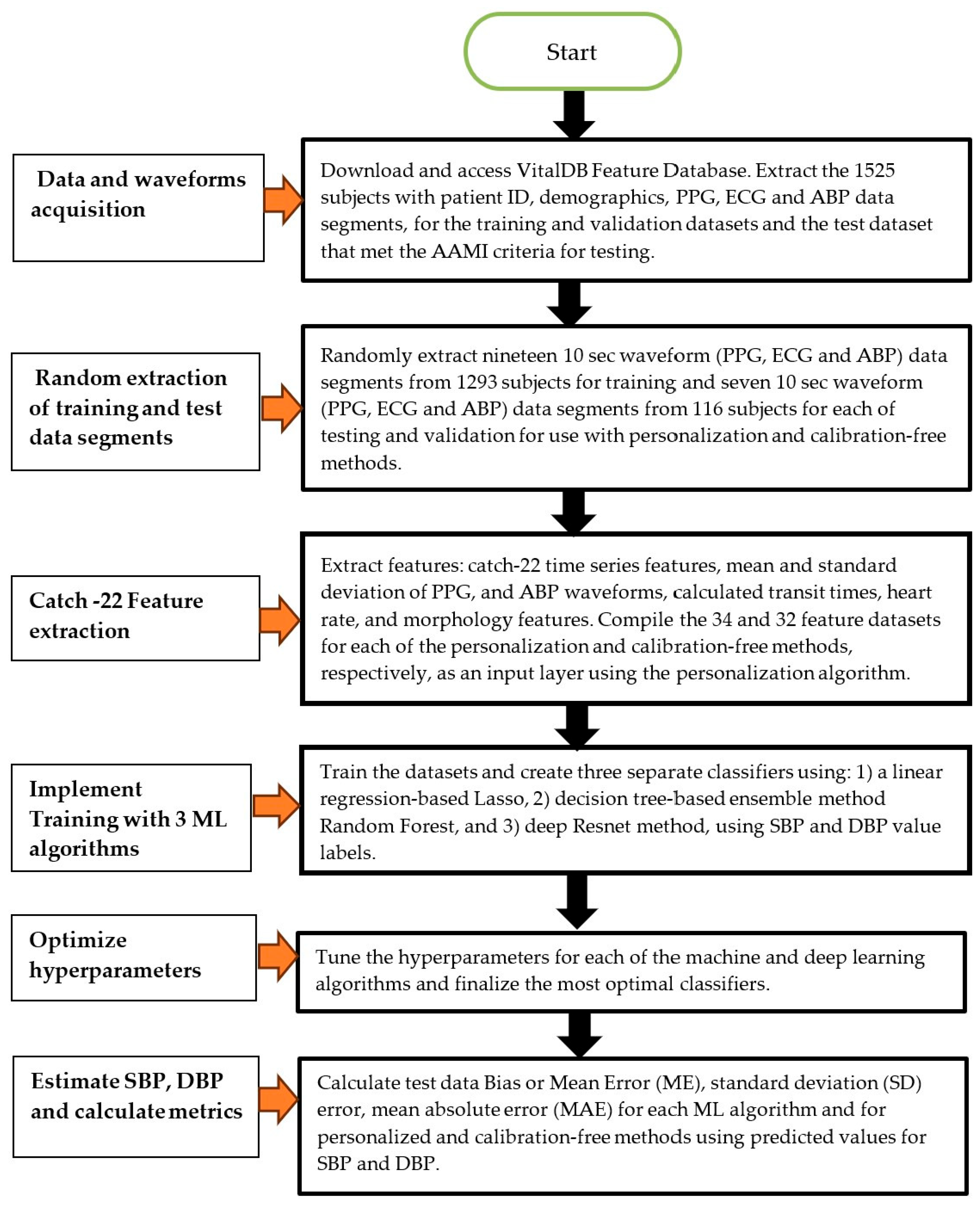
2. Methods
2.1. Human Data Ethical Statement
2.2. Patient Data
2.3. Feature Extraction
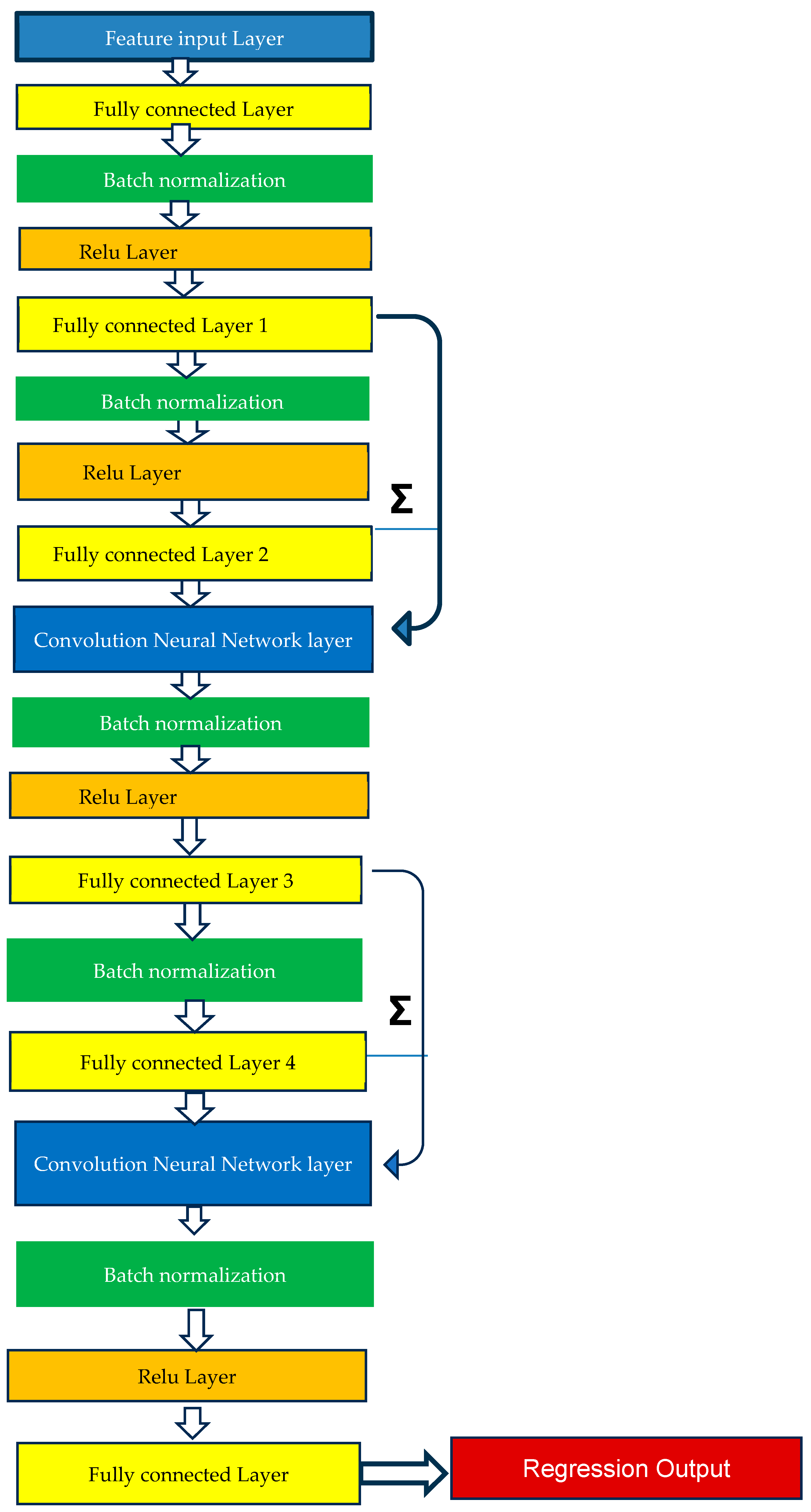
2.4. Method of Analysis—Machine Learning Model Training
2.5. Method of Analysis—Personalized and Calibration-Free Model Testing
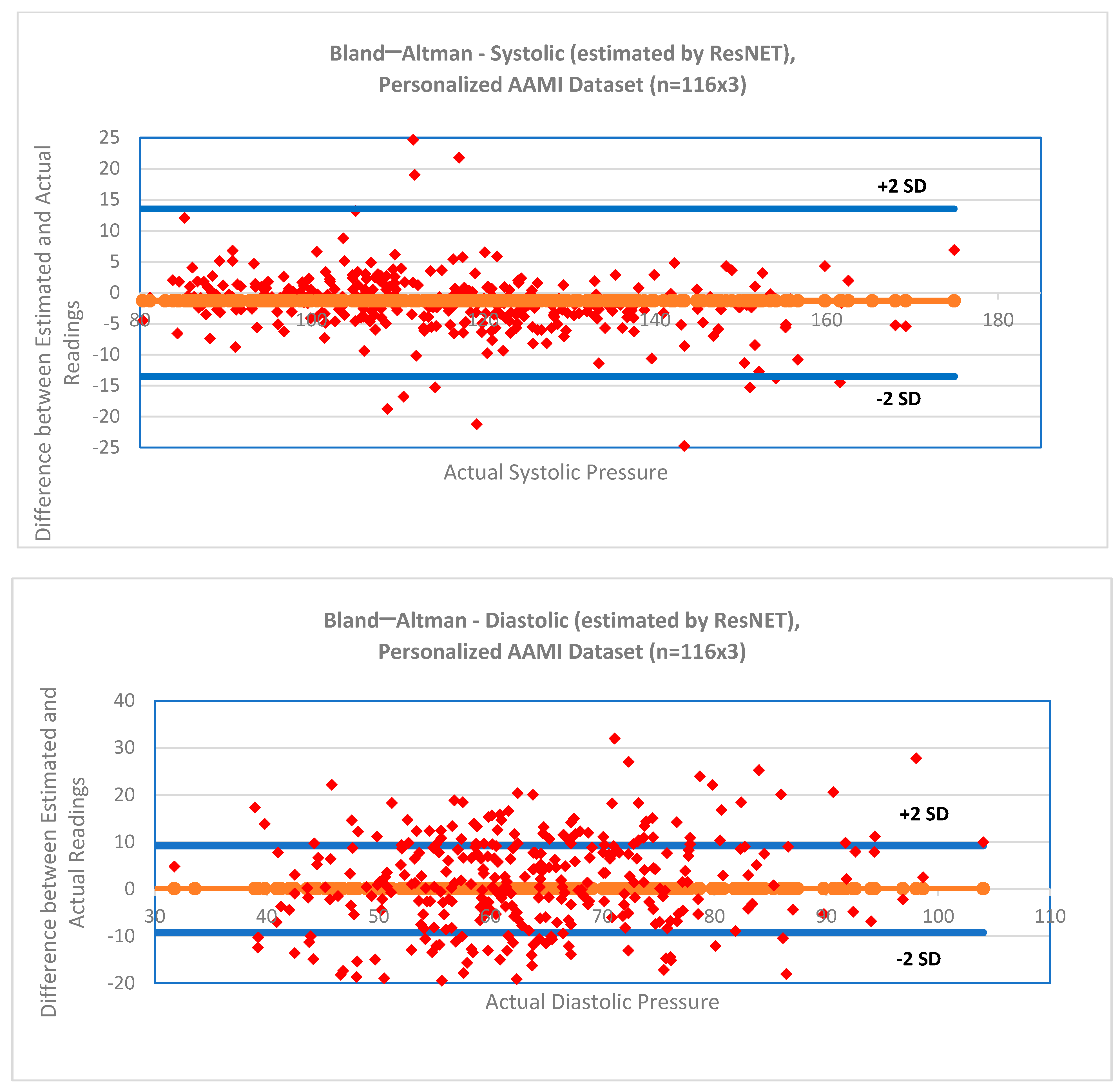
2.6. Statistical Analysis
3. Results
4. Discussion
Author Contributions
Funding
Institutional Review Board Statement
Informed Consent Statement
Data Availability Statement
Acknowledgments
Conflicts of Interest
Appendix A. Catch-22 Detailed Description

| # | Feature Name | Description |
|---|---|---|
| I. | Distribution-related features | |
| 1 | DN_HistogramMode_5 | Mode of z-scored distribution (5-bin histogram) |
| 2 | DN_HistogramMode_10 | Mode of z-scored distribution (10-bin histogram) |
| II. | Simple temporal statistics | |
| 3 | SB_BinaryStats_mean_longstretch1 | Longest period of consecutive values above the mean |
| 4 | DN_OutlierInclude_p_001_mdrmd | Time intervals between successive extreme events above the mean |
| 5 | DN_OutlierInclude_n_001_mdrmd | Time intervals between successive extreme events below the mean |
| III. | Linear autocorrelation | |
| 6 | CO_flecac | First 1/e crossing of autocorrelation function |
| 7 | CO_FirstMin_ac | First minimum of autocorrelation function |
| 8 | SP_Summaries_welch_rect_area_5_1 | Total power in lowest fifth of frequencies in the Fourier power spectrum |
| 9 | SP_Summaries_welch_rect_centroid | Centroid of the Fourier power spectrum |
| 10 | FC_LocalSimple_mean3_stderr | Mean error from a rolling 3-sample mean forecasting |
| IV. | Non-linear autocorrelation | |
| 11 | CO_trev_1_num | Time reversibility statistic |
| 12 | CO_HistogramAMI_even_2_5 | Automutual information, m = 2, r = 5 |
| 13 | IN_AutoMutualInfoStats_40_gaussian_fnni | First minimum of the automutual information function |
| V. | Successive differences | |
| 14 | MD_hrv_classic_pnn40 | Proportion of successive differences exceeding 0.04σ |
| 15 | SB_BinaryStats_mean_longstretch0 | Longest period of successive incremental decreases |
| 16 | SB_MotifThree_quantile_hh | Shannon entropy of two successive letters in equiprobable 3-letter symbolization |
| 17 | FC_LocalSimple_mean3_stderr | Change in correlation length after iterative differencing |
| 18 | CO_embed2_Dist_tau_d_expfit_meandiff | Exponential fit to successive distances in 2-d embedding space |
| VI. | Fluctuation analysis | |
| 19 | SC_FlucAnal_2_dfa_50_1_2_logi_prop_r1 | Proportion of slower timescale fluctuations that scale with DFA (50% sampling) |
| 20 | SC_FlucAnal_2_rsrangefit_50_1_logi_prop_r1 | Proportion of slower timescale fluctuations that scale with linearly rescaled range fits |
| V | Others | |
| 21 | SB_TransitionMatrix_3ac_sumdiagcov | Trace of covariance of transition matrix between symbols in 3-letter alphabet |
| 22 | PD_PeriodicityWang_th0_01 | Periodicity measure |
References
- Zhao, L.; Liang, C.; Huang, Y.; Zhou, G.; Xiao, Y.; Ji, N.; Zhang, Y.T.; Zhao, N. Emerging sensing and modeling technologies for wearable and cuffless blood pressure monitoring. NPJ Digit. Med. 2023, 6, 93. [Google Scholar] [CrossRef] [PubMed]
- Allen, J. Photoplethysmography and its application in clinical physiological measurement. Physiol. Meas. 2007, 28, R1–R39. [Google Scholar] [CrossRef] [PubMed]
- Kario, K.; Hoshide, S.; Mizuno, H.; Kabutoya, T.; Nishizawa, M.; Yoshida, T.; Abe, H.; Katsuya, T.; Fujita, Y.; Okazaki, O.; et al. Nighttime blood pressure phenotype and cardiovascular prognosis: Practitioner-based nationwide JAMP study. Circulation 2020, 142, 1810–1820. [Google Scholar] [CrossRef] [PubMed]
- Parati, G. Nocturnal Hypertension and associated mechanisms. In Proceedings of the 32nd European Meeting on Hypertension and Cardiovascular Protection, Milan, Italy, 23–26 June 2023. [Google Scholar]
- Mukkamalla, S.K.R.; Kashyap, S.; Recio-Boiles, A.; Babiker, H.M. Gallbladder Carcinoma. In StatPearls; StatPearls Publishing: Treasure Island, FL, USA, 2023. [Google Scholar]
- Sola, A.M.; David, A.P.; Rosbe, K.W.; Baba, A.; Ramirez-Avila, L.; Chan, D.K. Prevalence of SARS-CoV-2 infection in children without symptoms of coronavirus disease 2019. JAMA Pediatr. 2021, 175, 198–201. [Google Scholar] [CrossRef]
- Stergiou, G.S.; Mukkamala, R.; Avolio, A.; Kyriakoulis, K.G.; Mieke, S.; Murray, A.; Parati, G.; Schutte, A.E.; Sharman, J.E.; Asmar, R.; et al. Cuffless blood pressure measuring devices: Review and statement by the European Society of Hypertension working group on blood pressure monitoring and cardiovascular variability. J. Hypertens. 2022, 40, 1449–1460. [Google Scholar] [CrossRef]
- The Aurora-BP Study and Dataset. Available online: https://github.com/microsoft/aurorabp-sample-data/ (accessed on 2 November 2022).
- Stergiou, G.S.; Avolio, A.P.; Palatini, P.; Kyriakoulis, K.G.; Schutte, A.E.; Mieke, S.; Kollias, A.; Parati, G.; Asmar, R.; Pantazis, N.; et al. European Society of Hypertension recommendations for the validation of cuffless blood pressure measuring devices. J. Hypertens. 2023, 12, 10–97. [Google Scholar]
- Tanveer, M.S.; Hasan, M.K. Cuffless blood pressure estimation from electrocardiogram and photoplethysmogram using waveform-based ANN-LSTM network. Biomed. Signal Process. Control 2019, 51, 382–392. [Google Scholar] [CrossRef]
- Eom, H.; Lee, D.; Han, S.; Hariyani, Y.S.; Lim, Y.; Sohn, I.; Park, K.; Park, C. End-To-End Deep Learning Architecture for Continuous Blood Pressure Estimation Using Attention Mechanism. Sensors 2020, 20, 2338. [Google Scholar] [CrossRef]
- Sadrawi, M.; Lin, Y.-T.; Lin, C.-H.; Mathunjwa, B.; Fan, S.-Z.; Abbod, M.F.; Shieh, J.-S. Genetic Deep Convolutional Autoencoder Applied for Generative Continuous Arterial Blood Pressure via Photoplethysmography. Sensors 2020, 20, 3829. [Google Scholar] [CrossRef]
- Athaya, T.; Choi, S. An Estimation Method of Continuous Non-Invasive Arterial Blood Pressure Waveform Using Photoplethysmography: A U-Net Architecture-Based Approach. Sensors 2021, 21, 1867. [Google Scholar] [CrossRef]
- Jeong, D.U.; Lim, K.M. Combined deep CNN-LSTM network-based multitasking learning architecture for noninvasive continuous blood pressure estimation using difference in ECG-PPG features. Sci. Rep. 2021, 11, 13539. [Google Scholar] [CrossRef] [PubMed]
- Fan, X.; Wang, H.; Zhao, Y.; Li, Y.; Tsui, K.L. An Adaptive Weight Learning-Based Multitask Deep Network for Continuous Blood Pressure Estimation Using Electrocardiogram Signals. Sensors 2021, 21, 1595. [Google Scholar] [CrossRef] [PubMed]
- Hu, Q.; Wang, D.; Yang, C. PPG-based blood pressure estimation can benefit from scalable multi-scale fusion neural networks and multi-task learning. Biomed. Signal Process. Control 2022, 78, 103891. [Google Scholar] [CrossRef]
- Ibtehaz, N.; Mahmud, S.; Chowdhury, M.E.H.; Khandakar, A.; Khan, M.S.; Ayari, M.A.; Tahir, A.M.; Rahman, M.S. PPG2ABP: Translating Photoplethysmogram (PPG) Signals to Arterial Blood Pressure (ABP) Waveforms. Bioengineering 2022, 9, 692. [Google Scholar] [CrossRef]
- Jiang, H.; Zou, L.; Huang, D.; Feng, Q. Continuous Blood Pressure Estimation Based on Multi-Scale Feature Extraction by the Neural Network with Multi-Task Learning. Front. Neurosci. 2022, 16, 883693. [Google Scholar] [CrossRef]
- Mahmud, S.; Ibtehaz, N.; Khandakar, A.; Tahir, A.M.; Rahman, T.; Islam, K.R.; Hossain, M.S.; Rahman, M.S.; Musharavati, F.; Ayari, M.A.; et al. A Shallow U-Net Architecture for Reliably Predicting Blood Pressure (BP) from Photoplethysmogram (PPG) and Electrocardiogram (ECG) Signals. Sensors 2022, 22, 919. [Google Scholar] [CrossRef]
- Seok, W.; Lee, K.J.; Cho, D.; Roh, J.; Kim, S. Blood Pressure Monitoring System Using a Two-Channel Ballistocardiogram and Convolutional Neural Networks. Sensors 2021, 21, 2303. [Google Scholar] [CrossRef]
- Treebupachatsakul, T.; Boosamalee, A.; Shinnakerdchoke, S.; Pechprasarn, S.; Thongpance, N. Cuff-Less Blood Pressure Prediction from ECG and PPG Signals Using Fourier Transformation and Amplitude Randomization Preprocessing for Context Aggregation Network Training. Biosensors 2022, 12, 159. [Google Scholar] [CrossRef]
- Kachuee, M.; Kiani, M.M.; Mohammadzade, H.; Shabany, M. Cuff-less high-accuracy calibration-free blood pressure estimation using pulse transit time. In Proceedings of the 2015 IEEE International Symposium on Circuits and Systems (ISCAS), Lisbon, Portugal, 24–27 May 2015; pp. 1006–1009. [Google Scholar]
- Mahardika, T.N.Q.; Fuadah, Y.N.; Jeong, D.U.; Lim, K.M. PPG Signals-Based Blood-Pressure Estimation Using Grid Search in Hyperparameter Optimization of CNN–LSTM. Diagnostics 2023, 13, 2566. [Google Scholar] [CrossRef]
- van Vliet, M.; Monnink, S.H.; Kuiper, M.J.; Constandse, J.C.; Hoftijzer, D.; Ronner, E. Evaluation of a novel cuffless photoplethysmography-based wristband for measuring blood pressure according to the regulatory standards. Eur. Heart J.—Digit. Health 2024, 5, 335–343. [Google Scholar] [CrossRef]
- Huang, Y.; Chen, L.; Li, C.; Peng, J.; Hu, Q.; Sun, Y.; Ren, H.; Lyu, W.; Jin, W.; Tian, J.; et al. AI-driven system for non-contact continuous nocturnal blood pressure monitoring using fiber optic ballistocardiography. Commun. Eng. 2024, 3, 183. [Google Scholar] [CrossRef] [PubMed]
- Liu, S.-H.; Sun, Y.; Wu, B.-Y.; Chen, W.; Zhu, X. Using machine learning models for cuffless blood pressure estimation with ballistocardiogram and impedance plethysmogram. Front. Digit. Health 2025, 7, 1511667. [Google Scholar] [CrossRef] [PubMed]
- Kasbekar, R.S.; Ji, S.; Clancy, E.A.; Goel, A. Optimizing the input feature sets and machine learning algorithms for reliable and accurate estimation of continuous, cuffless blood pressure. Sci. Rep. 2023, 13, 7750. [Google Scholar] [CrossRef] [PubMed]
- Elgendi, M. Optimal signal quality index for photoplethysmogram signals. Bioengineering 2016, 3, 21. [Google Scholar] [CrossRef]
- Kasbekar, R.S.; Mendelson, Y. Evaluation of key design parameters for mitigating motion artefact in the mobile reflectance PPG signal to improve estimation of arterial oxygenation. Physiol. Meas. 2018, 39, 075008. [Google Scholar] [CrossRef]
- Wang, W.; Mohseni, P.; Kilgore, K.L.; Najafizadeh, L. PulseDB: A large, cleaned dataset based on MIMIC-III and VitalDB for benchmarking cuff-less blood pressure estimation methods. Front. Digit. Health 2023, 4, 1090854. [Google Scholar] [CrossRef]
- Lee, H.-C.; Park, Y.; Yoon, S.B.; Yang, S.M.; Park, D.; Jung, C.-W. VitalDB, a high-fidelity multi-parameter vital signs database in surgical patients. Sci. Data 2022, 9, 1–9. [Google Scholar] [CrossRef]
- Pan, J.; Tompkins, W.J. A real-time QRS detection algorithm. IEEE Trans. Biomed. Eng. 1985, 32, 230–236. [Google Scholar] [CrossRef]
- Elgendi, M.; Norton, I.; Brearley, M.; Abbott, D.; Schuurmans, D. Systolic peak detection in acceleration photoplethysmograms measured from emergency responders in tropical conditions. PLoS ONE 2013, 8, e76585. [Google Scholar] [CrossRef]
- IEC/AAMI 80601-2-30:2018; Medical Electrical Equipment—Part 2–30: Requirements for Basic Safety and Essential Performance of Automated Non-Invasive Sphygmomanometers. International Electrotechnical Commission (IEC): Geneva, Switzerland, 2018.
- Lubba, C.H.; Sethi, S.S.; Knaute, P.; Schultz, S.R.; Fulcher, B.D.; Jones, N.S. catch22: CAnonical Time-series CHaracteristics: Selected through highly comparative time-series analysis. Data Min. Knowl. Discov. 2019, 33, 1821–1852. [Google Scholar] [CrossRef]
- Bland, J.M.; Altman, D.G. Statistical methods for assessing agreement between two methods of clinical measurement. Lancet 1986, 327, 307–310. [Google Scholar] [CrossRef]
- O’Brien, E.; Petrie, J.; Littler, W.; de Swiet, M.; Padfield, P.L.; Altman, D.G.; Bland, M.; Coats, A.; Atkins, N. An outline of the revised British Hypertension Society protocol for the evaluation of blood pressure measuring devices. J. Hypertens. 1993, 11, 677–679. [Google Scholar] [CrossRef] [PubMed]
- Schrumpf, F.; Frenzel, P.; Aust, C.; Osterhoff, G.; Fuchs, M. Assessment of Non-Invasive Blood Pressure Prediction from PPG and rPPG Signals Using Deep Learning. Sensors 2021, 21, 6022. [Google Scholar] [CrossRef] [PubMed]
- Leitner, J.J.; Chiang, P.-H.; Dey, S. Personalized blood pressure estimation using photoplethysmography: A transfer learning approach. IEEE J. Biomed. Health Inform. 2022, 26, 218–228. [Google Scholar] [CrossRef]
- Bresch, E.; Derkx, R.; Paulussen, I.; Noordergraaf, G.J.; Schmitt, L.; Muehlsteff, J. Personalization of pulse arrival time-based blood pressure surrogates through single spot check measurements. In Proceedings of the 2021 43rd Annual International Conference of the IEEE Engineering in Medicine & Biology Society (EMBC), Guadalajara, Mexico, 1–5 November 2021; pp. 5437–5440. [Google Scholar]
- Samartkit, P.; Pullteap, S.; Bernal, O. A non-invasive heart rate and blood pressure monitoring system using piezoelectric and photoplethysmographic sensors. Measurement 2022, 196, 111211. [Google Scholar] [CrossRef]
- Lin, Q.; Huang, J.; Yang, J.; Huang, Y.; Zhang, Y.; Wang, Y.; Zhang, J.; Wang, Y.; Yuan, L.; Cai, M.; et al. Highly sensitive flexible iontronic pressure sensor for fingertip pulse monitoring. Adv. Healthc. Mater. 2020, 9, 2001023. [Google Scholar] [CrossRef]
- Nichols, W.W. Clinical measurement of arterial stiffness obtained from noninvasive pressure waveforms. Am. J. Hypertens. 2005, 18, 3S–10S. [Google Scholar] [CrossRef]
| Authors | Year | Sensor Signal | Method Used | Sample Size | Data Source | Study Duration | Mean ± SD Errors (mm Hg) |
|---|---|---|---|---|---|---|---|
| Tanveer et al. | [10]/2019 | ECG, PPG | Artificial neural network-long short-term memory network | 39 (hemodynamically compromised) | Prospective | Short term (40 s) | SBP: 1.10 (MAE) DBP: 0.58 (MAE) |
| Eom et al. | [11]/2020 | PPG | Convolution neural network and bi-directional gated recurrent network | 15 (healthy) | Prospective | Short term (<1 h) | SBP: −0.20 ± 5.83 DBP: −0.02 ± 4.91 |
| Sadrawi et al. | [12]/2020 | PPG | Genetic deep convolution autoencoder | 18 (healthy, hemodynamically compromised) | Prospective | Short term (<6 h) | SBP: −1.66 ± 7.496 DBP: 0.66 ± 3.31 |
| Athaya et al. | [13]/2021 | PPG | U-net deep learning architecture | 100 (hemodynamically compromised) | MIMIC, MIMIC III | Short term (3.4 h) | SBP: 3.68 ± 4.42 DBP: 1.97 ± 2.92 MAP: 2.17 ± 3.06 |
| Jeong et al. | [14]/2021 | ECG, PPG | Convolution neural network-long short-term memory combination | 48 (healthy) | Prospective | Short Term (<800 s) | SBP: 0.2 ± 1.3 DBP: 0.0 ± 1.6 |
| Fan et al. | [15]/2021 | ECG | Bi-layer long short-term memory network | 942 (hemodynamically compromised) | MIMIC II | Short Term (~230 s) | SBP: 7.69 ±10.83 DBP: 4.36 ± 5.90 MAP: 4.76 ± 6.47 |
| Hu Q et al. | [16]/2022 | PPG | Convolution neural network with attention mechanism, multi-task learning | 1825 (hemodynamically compromised) | UC, Irvine database | Short Term (<20 min) | SBP: 0.97 ± 8.87 DBP: 0.55 ± 4.23 |
| Ibtehaz et al. | [17]/2022 | PPG | Two-stage cascaded convolution neural network | 942 (healthy and hemodynamically compromised) | MIMIC III | Short Term (<30 min) | SBP: 5.7 ± 9.2 DBP: 3.4 ± 6.1 MAP: 2.3 ± 4.4 |
| Jiang et al. | [18]/2022 | ECG, PPG | Neural network with multi-task learning | 3000 (hemodynamically compromised) | MIMIC-II | Short Term (60 h) | SBP: 4.04 ± 5.8 DBP: 2.29 ± 3.55 MAP: 2.46 ± 3.58 |
| Mahmud et al. | [19]/2022 | ECG, PPG | Shallow one-dimensional auto-encoder (U-net architecture) | 942 (hemodynamically compromised) | MIMIC II | Short Term (<21 min) | SBP: 2.73 (MAE) DBP: 1.17 (MAE) |
| Seok et al. | [20]/2021 | BCG | Convolution neural network | 30 (healthy) | Prospective | Short Term (<10 s) | SBP: 0.93 ± 6.24 DBP: 0.21 ± 5.42 |
| Treebupachatsakul et al. | [21]/2022 | ECG, PPG | Fourier transformation followed by deep learning | >2500 (healthy and hemodynamically compromised) | Kachuee et al., 2015 [22] | Short Term (<30 min) | SBP: 7 DBP: 6 |
| Mahardika et al. | [23]/2023 | PPG, ABP | Convolution neural network, long short-term memory network | 55 | MIMIC-III | Short Term (<5 min) | SBP: 0.13 ± 7.04 DBP: 0.48 ± 3.79 |
| Vliet et al. | [24]/2024 | PPG | Machine learning algorithm—exact method not disclosed | 124 | Prospective | Short Term (<30 s) | SBP: ±3.7 ± 4.4 DBP: ±2.5 ± 3.7 |
| Huang et al. | [25]/2024 | BCG | Deep learning UUNet | 40 (nighttime) | Kansas dataset | Short term (<30 min) | SBP: −0.19 ± 8.31 DBP: −0.04 ± 4.48 |
| Liu et al. | [26]/2025 | BCG, IPG | Random forest, XGBoost | 17 | Prospective (healthy) | Short term (<18 min) | SBP, MAD: 3.54 DBP, MAD: 2.57 |
| Lasso | Random Forest | ResNET | |
|---|---|---|---|
| Type | Machine Learning | Machine Learning | Deep Learning |
| Principle | Based on least square multiple regression adjusted for overfitting | Based on an ensemble of decision trees based on bagging or boosting these trees | Based on multiple layers (18) of convolution neural networks with batch normalization and ReLU activation function |
| Cross-validation | Yes—10-fold | Yes—10-fold | Yes—5-fold |
| Complexity | Low | Medium | High |
| Hyperparameter | Alpha—Lasso to ridge ratio | Learning rate, leaf size, learning cycles, splits and features to sample | Number of epochs, learning rate |
| Computation time | Low | High | High |
| Input feature type | Binary, numerical | Binary, numerical | Binary, numerical, and categorical |
| Fit parameters | 100 | 492 | 840 |
| Data amount (>10 times fit parameter) | Can work with relatively less data | Needs more data for effective performance | Needs large amounts of data |
| Descriptor | Training Subjects | Validation Subjects | Test Subjects |
|---|---|---|---|
| Male | 751 (58%) | 69 (59%) | 69 (59%) |
| Female | 542 (42%) | 47 (41%) | 47 (41%) |
| Age (>40 years) | 1137 (88%) | 103 (89%) | 103 (89%) |
| Total | 1293 | 116 | 116 |
| (a) | ||||||
| Lasso | Random Forest | ResNET | ||||
| μ ± SD | (MAE) | μ ± SD | (MAE) | μ ± SD | (MAE) | |
| SBP | −2.11 ± 18.78 | 14.25 | −1.08 ± 18.76 | 14.20 | −1.86 ± 19.55 | 14.69 |
| DBP | −0.68 ± 11.77 | 9.18 | −0.24 ± 11.06 | 8.56 | 0.11 ± 11.55 | 9.06 |
| (b) | ||||||
| Lasso | Random Forest | ResNET | ||||
| μ ± SD | (MAE) | μ ± SD | (MAE) | μ ± SD | (MAE) | |
| SBP * | −1.51 ± 8.04 | 4.88 | −1.32 ± 7.97 | 4.95 | −1.31 ± 7.91 | 4.83 |
| DBP * | −0.52 ± 4.69 | 2.62 | −0.43 ± 4.62 | 2.60 | 0.10 ± 4.59 | 2.65 |
| (c) | ||||||
| Absolute Difference | ||||||
| ≤5 mm Hg | ≤10 mm Hg | ≤15 mm Hg | Grade | |||
| BHS Standard | SBP, DBP | 60% | 85% | 95% | A | |
| 50% | 75% | 90% | B | |||
| 40% | 65% | 80% | C | |||
| Worse than C | D | |||||
| Proposed Model: Personalized, ResNET | SBP | 65.8% | 91.7% | 95% | A | |
| DBP | 85.9% | 96.8% | 98.6% | A | ||
| Method | SBP | DBP |
|---|---|---|
| F-Statistic, p-Value | F-Statistic, p-Value | |
| Machine Learning Algorithm | F(1) = 0.00, 0.99 | F(1) = 0.19, 0.82 |
| Method (Calibration-free vs. Personalized) | F(2) = 45.9, 0.00 | F(2) = 46.9, 0.00 |
| Method | Systolic BP Estimation Errors | Diastolic BP Estimation Errors | ||||
|---|---|---|---|---|---|---|
| Bias | SD | MAE | Bias | SD | MAE | |
| Estimated by algorithm (in mm Hg) | −1.31 | 7.91 | 4.83 | 0.10 | 4.59 | 2.65 |
| Estimated using ”ground truth” (in mm Hg) | −1.21 | 19.46 | 14.75 | −0.40 | 13.68 | 9.87 |
| p-values and F-statistic, bias (ANOVA) | F = 1.28, p = 0.26 | F = 2.06, p = 0.15 | ||||
| p-values and F-statistic, variance (Levene’s test) | F = 91.42, p = 0.00 | F = 99.04, p = 0.00 | ||||
Disclaimer/Publisher’s Note: The statements, opinions and data contained in all publications are solely those of the individual author(s) and contributor(s) and not of MDPI and/or the editor(s). MDPI and/or the editor(s) disclaim responsibility for any injury to people or property resulting from any ideas, methods, instructions or products referred to in the content. |
© 2025 by the authors. Licensee MDPI, Basel, Switzerland. This article is an open access article distributed under the terms and conditions of the Creative Commons Attribution (CC BY) license (https://creativecommons.org/licenses/by/4.0/).
Share and Cite
Kasbekar, R.S.; Radhakrishnan, S.; Ji, S.; Goel, A.; Clancy, E.A. Optimizing Input Feature Sets Using Catch-22 and Personalization for an Accurate and Reliable Estimation of Continuous, Cuffless Blood Pressure. Bioengineering 2025, 12, 493. https://doi.org/10.3390/bioengineering12050493
Kasbekar RS, Radhakrishnan S, Ji S, Goel A, Clancy EA. Optimizing Input Feature Sets Using Catch-22 and Personalization for an Accurate and Reliable Estimation of Continuous, Cuffless Blood Pressure. Bioengineering. 2025; 12(5):493. https://doi.org/10.3390/bioengineering12050493
Chicago/Turabian StyleKasbekar, Rajesh S., Srinivasan Radhakrishnan, Songbai Ji, Anita Goel, and Edward A. Clancy. 2025. "Optimizing Input Feature Sets Using Catch-22 and Personalization for an Accurate and Reliable Estimation of Continuous, Cuffless Blood Pressure" Bioengineering 12, no. 5: 493. https://doi.org/10.3390/bioengineering12050493
APA StyleKasbekar, R. S., Radhakrishnan, S., Ji, S., Goel, A., & Clancy, E. A. (2025). Optimizing Input Feature Sets Using Catch-22 and Personalization for an Accurate and Reliable Estimation of Continuous, Cuffless Blood Pressure. Bioengineering, 12(5), 493. https://doi.org/10.3390/bioengineering12050493