
Stroke Lesion Segmentation and Deep Learning: A Comprehensive Review

 , ,
, , 
 and
and 
Abstract

1. Introduction

| Aspect | MRI | CT |
|---|---|---|
| Time Constraints | An MRI scan may require up to an hour to conclude its findings [15]. However, some medical centres have reduced the time to up to 10 min using different protocols [16]. | A CT typically takes between 5 and 15 min per scan. |
| Cost Effective | MRI costs almost double compared to a CT [17]. | A CT costs half the amount of an MRI [17]. |
| Ischaemic Lesion Detection | Since MRI scans produce detailed images, detecting small lesions is easier [18]. | CT scans are good at detecting large ischaemic lesions. It might be challenging to catch a small lesion earlier using a CT scan [18]. |
| Haemorrhage Detection | MRI scans are suitable for detecting small or chronic haemorrhages [18]. | CT scans perform well while detecting acute or larger haemorrhages. [19]. |
| Lesion Visibility | As an MRI produces a more detailed image, it is easier to detect and visualise a lesion. A lesion is more evident in the hyperintense region using a DWI map [20]. | Due to low contrast, a lesion is harder to visualise in a CT scan [20]. |
| Easier segmentation | It is easier to segment a lesion using an MRI scan manually. The different modalities, such as DWI, FLAIR, and T2-weighted, can be used to perform segmentation more accurately [21]. | Due to the low tissue contrast, it is harder to manually segment a lesion using a CT scan [21]. |
| Health Concerns | The magnetic rays emitted by the MRI scanner can disrupt the working of different implanted devices. | Since CT scanners use ionising radiation, they can cause cellular damage. |
2. Previous Literature Surveys
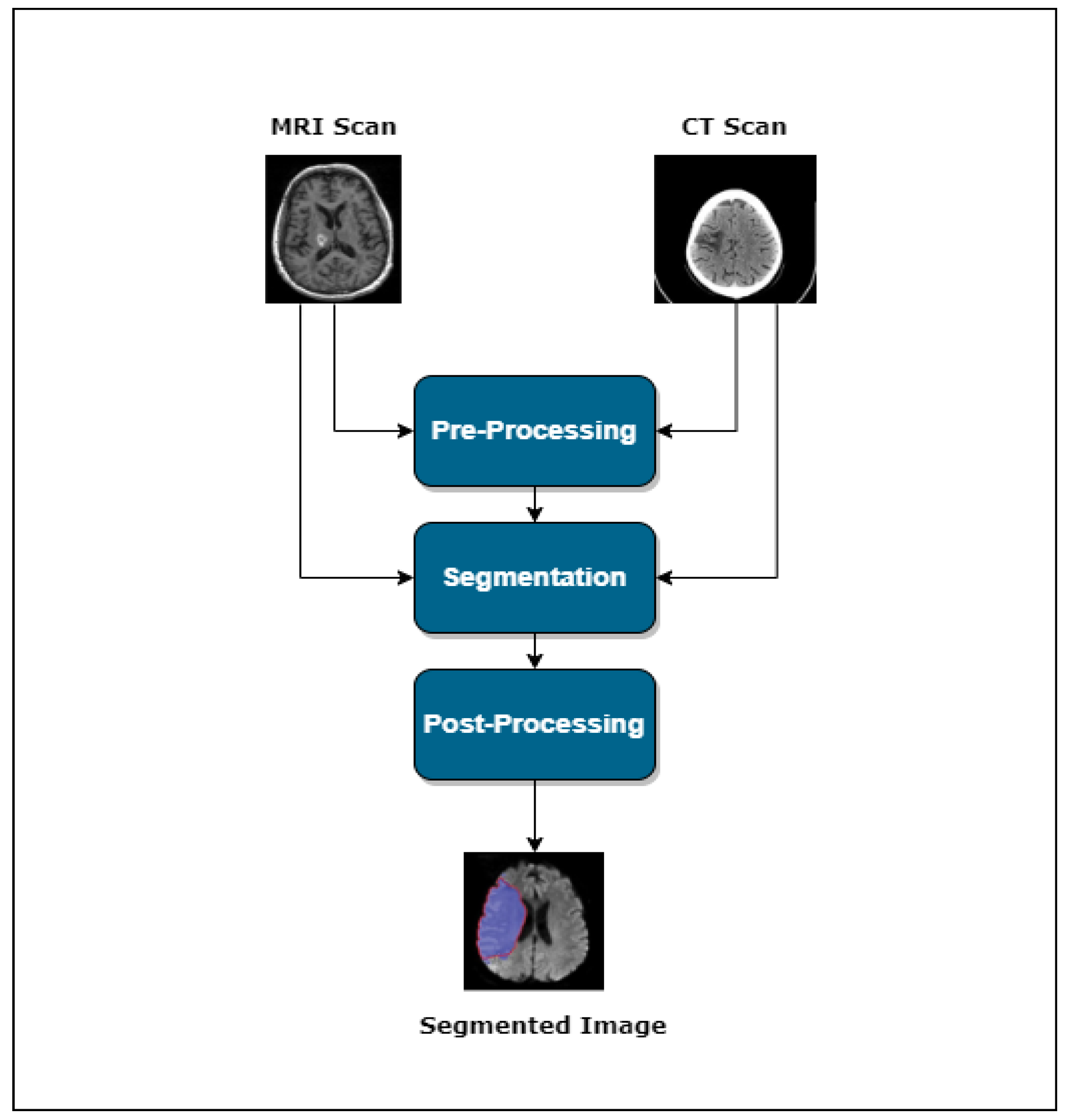
3. Stroke Lesion Segmentation
- Pre-processing
- Segmentation
- Post-processing
3.1. The Role of Pre-Processing in Stroke Lesion Segmentation
3.2. Advancements and Diverse Architectures in Automated Lesion Segmentation
3.2.1. Supervised Learning
3.2.2. Semi-Supervised Learning
3.2.3. Unsupervised Learning
4. Results and Future Directions
4.1. Data Dimensionality and Its Processing Techniques
4.2. Data Pre-Processing
4.3. Data Augmentation Trends
4.4. Enhancing Segmentation Using Transfer Learning
5. Limitations
6. Conclusions
Supplementary Materials
Author Contributions
Funding
Institutional Review Board Statement
Acknowledgments
Conflicts of Interest
References
- Feigin, V.L.; Owolabi, M.O.; Abanto, C.; Addissie, A.; Adeleye, A.O.; Adilbekov, Y.; Topcuoglu, M.A. Pragmatic Solutions to Reduce the Global Burden of Stroke: A World Stroke Organization—Lancet Neurology Commission. Lancet Neurol. 2023, 10, 142–149. [Google Scholar] [CrossRef] [PubMed]
- Feigin, V.L.; Brainin, M.; Norrving, B.; Martins, S.; Sacco, R.L.; Hacke, W.; Lindsay, P. World Stroke Organization (WSO): Global Stroke Fact Sheet 2022. Int. J. Stroke 2022, 17, 18–29. [Google Scholar] [CrossRef]
- Ortiz, G.A.; Sacco, R.L. National Institutes of Health Stroke Scale (NIHSS). In Wiley Encyclopedia of Clinical Trials; D’Agostino, R.B., Sullivan, L., Massaro, J., Eds.; Wiley-Interscience: Hoboken, NJ, USA, 2008; pp. 1–9. [Google Scholar]
- Kothari, R.U.; Pancioli, A.; Liu, T.; Brott, T.; Broderick, J. Cincinnati Prehospital Stroke Scale: Reproducibility and Validity. Ann. Emerg. Med. 1999, 33, 373–378. [Google Scholar] [CrossRef]
- Wang, J.; Zhu, H.; Wang, S.H.; Zhang, Y.D. A Review of Deep Learning on Medical Image Analysis. Mob. Netw. Appl. 2021, 26, 351–380. [Google Scholar] [CrossRef]
- Zhang, Y.; Liu, S.; Li, C.; Wang, J. Application of Deep Learning Method on Ischemic Stroke Lesion Segmentation. J. Shanghai Jiaotong Univ. (Sci.) 2022, 27, 99–111. [Google Scholar] [CrossRef]
- Chen, C.; Yuan, K.; Fang, Y.; Bao, S.; Tong, R.K.Y. Hierarchically Spatial Encoding Module for Chronic Stroke Lesion Segmentation. In Proceedings of the 2021 10th International IEEE/EMBS Conference on Neural Engineering (NER), Virtual Conference, 10–13 May 2021; pp. 1000–1003. [Google Scholar]
- Pieper, S.; Halle, M.; Kikinis, R. 3D Slicer. In Proceedings of the 2004 2nd IEEE International Symposium on Biomedical Imaging: Nano to Macro (IEEE Cat No. 04EX821), Arlington, VA, USA, 18 April 2004; Volume 1, pp. 632–635. [Google Scholar]
- Yushkevich, P.A.; Gao, Y.; Gerig, G. ITK-SNAP: An interactive tool for semi-automatic segmentation of multi-modality biomedical images. In Proceedings of the 2016 38th Annual International Conference of the IEEE Engineering in Medicine and Biology Society (EMBC), Orlando, FL, USA, 16–20 August 2016; pp. 3342–3345. [Google Scholar]
- Stalling, D.; Westerhoff, M.; Hege, H.C. Amira: A Highly Interactive System for Visual Data Analysis. Visualization 2005, 38, 749–767. [Google Scholar]
- McAuliffe, M.J.; Lalonde, F.M.; McGarry, D.; Gandler, W.; Csaky, K.; Trus, B.L. Medical image processing, analysis and visualization in clinical research. In Proceedings of the 14th IEEE Symposium on Computer-Based Medical Systems, CBMS 2001, Bethesda, MD, USA, 26–27 July 2001; pp. 381–386. [Google Scholar]
- Zhang, X.; Xu, H.; Liu, Y.; Liao, J.; Cai, G.; Su, J.; Song, Y. A Multiple Encoders Network for Stroke Lesion Segmentation. In Proceedings of the Chinese Conference on Pattern Recognition and Computer Vision (PRCV), Virtual Conference, 29 October–1 November 2021; Springer International Publishing: Cham, Switzerland, 2021; pp. 524–535. [Google Scholar]
- Li, C. Stroke Lesion Segmentation with Visual Cortex Anatomy Alike Neural Nets. arXiv 2021, arXiv:2105.06544. [Google Scholar]
- Cerdá-Alberich, L.; Solana, J.; Mallol, P.; Ribas, G.; García-Junco, M.; Alberich-Bayarri, A.; Marti-Bonmati, L. MAIC—10 brief quality checklist for publications using artificial intelligence and medical images. Insights Imaging 2023, 14, 11. [Google Scholar] [CrossRef]
- Birenbaum, D.; Bancroft, L.W.; Felsberg, G.J. Imaging in Acute Stroke. West. J. Emerg. Med. 2011, 12, 67–76. [Google Scholar]
- Provost, C.; Soudant, M.; Legrand, L.; Hassen, W.B.; Xie, Y.; Soize, S.; Bourcier, R.; Benzakoun, J.; Edjlali, M.; Boulouis, G.; et al. Magnetic Resonance Imaging or Computed Tomography Before Treatment in Acute Ischemic Stroke: Effect on Workflow and Functional Outcome. Stroke 2019, 50, 659–664. [Google Scholar] [CrossRef]
- Tatlisumak, T. Is CT or MRI the Method of Choice for Imaging Patients with Acute Stroke? Why Should Men Divide if Fate Has United? Stroke 2002, 33, 2144–2145. [Google Scholar] [CrossRef]
- Vitali, P.; Savoldi, F.; Segati, F.; Melazzini, L.; Zanardo, M.; Fedeli, M.P.; Benedek, A.; Di Leo, G.; Menicanti, L.; Sardanelli, F. MRI versus CT in the Detection of Brain Lesions in Patients with Infective Endocarditis Before or After Cardiac Surgery. Neuroradiology 2022, 64, 905–913. [Google Scholar] [CrossRef]
- Vymazal, J.; Rulseh, A.M.; Keller, J.; Janouskova, L. Comparison of CT and MR imaging in ischemic stroke. Insights Imaging 2012, 3, 619–627. [Google Scholar] [CrossRef] [PubMed]
- Rubin, J.; Abulnaga, S.M. CT-To-MR conditional generative adversarial networks for ischemic stroke lesion segmentation. In Proceedings of the 2019 IEEE International Conference on Healthcare Informatics (ICHI), Xi’an, China, 10–13 June 2019; pp. 1–7. [Google Scholar]
- Muir, K.W.; Buchan, A.; von Kummer, R.; Rother, J.; Baron, J.C. Imaging of Acute Stroke. Lancet Neurol. 2006, 5, 755–768. [Google Scholar] [CrossRef] [PubMed]
- Rani, S.; Singh, B.K.; Koundal, D.; Athavale, V.A. Localization of stroke lesion in MRI images using object detection techniques: A comprehensive review. Neurosci. Inform. 2022, 2, 100070. [Google Scholar] [CrossRef]
- Girshick, R.; Donahue, J.; Darrell, T.; Malik, J. Rich feature hierarchies for accurate object detection and semantic segmentation. In Proceedings of the IEEE Conference on Computer Vision and Pattern Recognition, Columbus, OH, USA, 23–28 June 2014; pp. 580–587. [Google Scholar]
- Redmon, J.; Divvala, S.; Girshick, R.; Farhadi, A. You only look once: Unified, real-time object detection. In Proceedings of the IEEE Conference on Computer Vision and Pattern Recognition, Las Vegas, NV, USA, 27–30 June 2016; pp. 779–788. [Google Scholar]
- Liu, W.; Anguelov, D.; Erhan, D.; Szegedy, C.; Reed, S.; Fu, C.Y.; Berg, A.C. SSD: Single Shot Multibox Detector. In Proceedings of the 14th European Conference on Computer Vision (ECCV 2016), Part I, Amsterdam, The Netherlands, 11–14 October 2016; Springer International Publishing: Cham, Switzerland, 2016; pp. 21–37. [Google Scholar]
- Tan, M.; Pang, R.; Le, Q.V. EfficientDet: Scalable and Efficient Object Detection. In Proceedings of the IEEE/CVF Conference on Computer Vision and Pattern Recognition, Virtual Conference, 13–19 June 2020; pp. 10781–10790. [Google Scholar]
- Karthik, R.; Menaka, R.; Johnson, A.; Anand, S. Neuroimaging and deep learning for brain stroke detection—A review of recent advancements and future prospects. Comput. Methods Programs Biomed. 2020, 197, 105728. [Google Scholar] [CrossRef]
- Thiyagarajan, S.K.; Murugan, K. A systematic review on techniques adapted for segmentation and classification of ischemic stroke lesions from brain MR images. Wirel. Pers. Commun. 2021, 118, 1225–1244. [Google Scholar] [CrossRef]
- Karthik, R.; Menaka, R. Computer-aided detection and characterization of stroke lesion—A short review on the current state-of-the-art methods. Imaging Sci. J. 2018, 66, 1–22. [Google Scholar] [CrossRef]
- Wang, X.; Fan, Y.; Zhang, N.; Li, J.; Duan, Y.; Yang, B. Performance of machine learning for tissue outcome prediction in acute ischemic stroke: A systematic review and meta-analysis. Front. Neurol. 2022, 13, 910259. [Google Scholar] [CrossRef]
- Abbasi, H.; Orouskhani, M.; Asgari, S.; Zadeh, S.S. Automatic Brain Ischemic Stroke Segmentation with Deep Learning: A Review. Neurosci. Inform. 2023, 3, 100145. [Google Scholar] [CrossRef]
- Styner, M.A.; Charles, H.C.; Park, J.; Gerig, G. Multisite Validation of Image Analysis Methods: Assessing Intra- and Intersite Variability. In Proceedings of the Medical Imaging 2002: Image Processing, San Diego, CA, USA, 23–28 February 2002; Volume 4684, pp. 278–286. [Google Scholar]
- Clèrigues, A.; Valverde, S.; Bernal, J.; Freixenet, J.; Oliver, A.; Lladó, X. Acute and sub-acute stroke lesion segmentation from multimodal MRI. Comput. Methods Programs Biomed. 2020, 194, 105521. [Google Scholar] [CrossRef]
- Soltanpour, M.; Greiner, R.; Boulanger, P.; Buck, B. Improvement of automatic ischemic stroke lesion segmentation in CT perfusion maps using a learned deep neural network. Comput. Biol. Med. 2021, 137, 104849. [Google Scholar] [CrossRef] [PubMed]
- Sheng, M.; Xu, W.; Yang, J.; Chen, Z. Cross-Attention and Deep Supervision UNet for Lesion Segmentation of Chronic Stroke. Front. Neurosci. 2022, 16, 836412. [Google Scholar] [CrossRef]
- Goshtasby, A.A. 2-D and 3-D Image Registration: For Medical, Remote Sensing, and Industrial Applications; John Wiley & Sons: Hoboken, NJ, USA, 2005. [Google Scholar]
- Brown, L.G. A survey of image registration techniques. Acm Comput. Surv. (CSUR) 1992, 24, 325–376. [Google Scholar] [CrossRef]
- Oliveira, F.P.; Tavares, J.M.R. Medical image registration: A review. Comput. Methods Biomech. Biomed. Eng. 2014, 17, 73–93. [Google Scholar] [CrossRef] [PubMed]
- Fu, Y.; Lei, Y.; Wang, T.; Curran, W.J.; Liu, T.; Yang, X. Deep learning in medical image registration: A review. Phys. Med. Biol. 2020, 65, 20TR01. [Google Scholar] [CrossRef] [PubMed]
- Hui, H.; Zhang, X.; Wu, Z.; Li, F. Dual-path attention compensation U-Net for stroke lesion segmentation. Comput. Intell. Neurosci. 2021, 2021, 7552185. [Google Scholar] [CrossRef] [PubMed]
- Liu, X.; Yang, H.; Qi, K.; Dong, P.; Liu, Q.; Liu, X.; Wang, R.; Wang, S. MSDF-Net: Multi-scale deep fusion network for stroke lesion segmentation. IEEE Access 2019, 7, 178486–178495. [Google Scholar] [CrossRef]
- Wu, Z.; Zhang, X.; Li, F.; Wang, S.; Huang, L.; Li, J. W-Net: A boundary-enhanced segmentation network for stroke lesions. Expert Syst. Appl. 2023, 230, 120637. [Google Scholar] [CrossRef]
- Isa, A.M.A.A.A.; Kipli, K.; Mahmood, M.H.; Jobli, A.T.; Sahari, S.K.; Muhammad, M.S.; Chong, S.K.; Al-Kharabsheh, B.N.I. A Review of MRI Acute Ischemic Stroke Lesion Segmentation. Int. J. Integr. Eng. 2020, 12, 117–127. [Google Scholar]
- Gao, Y.; Li, J.; Xu, H.; Wang, M.; Liu, C.; Cheng, Y.; Li, M.; Yang, J.; Li, X. A multi-view pyramid network for skull stripping on neonatal T1-weighted MRI. Magn. Reson. Imaging 2019, 63, 70–79. [Google Scholar] [CrossRef]
- Tsai, C.; Manjunath, B.S.; Jagadeesan, B. Automated segmentation of brain MR images. Pattern Recognit. 1995, 28, 1825–1837. [Google Scholar] [CrossRef]
- Atkins, M.S.; Mackiewich, B.T. Fully automatic segmentation of the brain in MRI. IEEE Trans. Med. Imaging 1998, 17, 98–107. [Google Scholar] [CrossRef] [PubMed]
- Cox, R.W. AFNI: Software for analysis and visualization of functional magnetic resonance neuroimages. Comput. Biomed. Res. 1996, 29, 162–173. [Google Scholar] [CrossRef] [PubMed]
- Roy, S.; Butman, J.A.; Pham, D.L.; Alzheimer’s Disease Neuroimaging Initiative. Robust skull stripping using multiple MR image contrasts insensitive to pathology. NeuroImage 2017, 146, 132–147. [Google Scholar] [CrossRef]
- Fatima, A.; Shahid, A.R.; Raza, B.; Madni, T.M.; Janjua, U.I. State-of-the-Art Traditional to the Machine-and Deep-Learning-Based Skull Stripping Techniques, Models, and Algorithms. J. Digit. Imaging 2020, 33, 1443–1464. [Google Scholar] [CrossRef]
- Hazarika, R.A.; Kharkongor, K.; Sanyal, S.; Maji, A.K. A comparative study on different skull stripping techniques from brain magnetic resonance imaging. In International Conference on Innovative Computing and Communications (ICICC) 2019, Volume 1; Springer: Singapore, 2019; pp. 279–288. [Google Scholar]
- Rehman, H.Z.U.; Hwang, H.; Lee, S. Conventional and deep learning methods for skull stripping in brain MRI. Appl. Sci. 2020, 10, 1773. [Google Scholar] [CrossRef]
- Anand, V.K.; Khened, M.; Alex, V.; Krishnamurthi, G. Fully automatic segmentation for ischemic stroke using CT perfusion maps. In Brainlesion: Glioma, Multiple Sclerosis, Stroke and Traumatic Brain Injuries: 4th International Workshop, BrainLes 2018, Held in Conjunction with MICCAI 2018, Granada, Spain, 16 September 2018; Revised Selected Papers, Part I; Springer International Publishing: Cham, Switzerland, 2019; pp. 328–334. [Google Scholar]
- Cui, W.; Liu, Y.; Li, Y.; Guo, M.; Li, Y.; Li, X.; Wang, T.; Zeng, X.; Ye, C. Semi-supervised brain lesion segmentation with an adapted mean teacher model. In Information Processing in Medical Imaging, Proceedings of the 26th International Conference, IPMI 2019, Hong Kong, China, 2–7 June 2019; Proceedings 26; Springer International Publishing: Cham, Switzerland, 2019; pp. 554–565. [Google Scholar]
- Karthik, R.; Gupta, U.; Jha, A.; Rajalakshmi, R.; Menaka, R. A deep supervised approach for ischemic lesion segmentation from multimodal MRI using Fully Convolutional Network. Appl. Soft Comput. 2019, 84, 105685. [Google Scholar] [CrossRef]
- Ahmad, P.; Jin, H.; Alroobaea, R.; Qamar, S.; Zheng, R.; Alnajjar, F.; Aboudi, F. MH UNet: A multi-scale hierarchical based architecture for medical image segmentation. IEEE Access 2021, 9, 148384–148408. [Google Scholar] [CrossRef]
- Tureckova, A.; Rodríguez-Sánchez, A.J. ISLES challenge: U-shaped convolutional neural network with dilated convolution for 3D stroke lesion segmentation. In Brainlesion: Glioma, Multiple Sclerosis, Stroke and Traumatic Brain Injuries, Proceedings of the 4th International Workshop, BrainLes 2018, Held in Conjunction with MICCAI 2018, Granada, Spain, 16 September 2018; Revised Selected Papers, Part I; Springer International Publishing: Cham, Switzerland, 2019; pp. 319–327. [Google Scholar]
- Song, S.; Zheng, Y.; He, Y. A review of methods for bias correction in medical images. Biomed. Eng. Rev. 2017, 1, 1–10. [Google Scholar] [CrossRef]
- Xu, Y.; Hu, S.; Du, Y. Bias correction of multiple MRI images based on an improved nonparametric maximum likelihood method. IEEE Access 2019, 7, 166762–166775. [Google Scholar] [CrossRef]
- Matsoukas, C.; Haslum, J.F.; Sorkhei, M.; Söderberg, M.; Smith, K. What makes transfer learning work for medical images: Feature reuse & other factors. In Proceedings of the IEEE/CVF Conference on Computer Vision and Pattern Recognition, New Orleans, LA, USA, 18–24 June 2022. [Google Scholar]
- Philipsen, R.H.; Maduskar, P.; Hogeweg, L.; Melendez, J.; Sánchez, C.I.; van Ginneken, B. Localized energy-based normalization of medical images: Application to chest radiography. IEEE Trans. Med. Imaging 2015, 34, 1965–1975. [Google Scholar] [CrossRef] [PubMed]
- Hong, G. Image Fusion, Image Registration and Radiometric Normalization for High-Resolution Image Processing. Ph.D. Thesis, University of New Brunswick, Fredericton, NB, Canada, 2023. [Google Scholar]
- Delisle, P.L.; Anctil-Robitaille, B.; Desrosiers, C.; Lombaert, H. Realistic image normalization for multi-domain segmentation. Med. Image Anal. 2021, 74, 102191. [Google Scholar] [CrossRef]
- Modanwal, G.; Vellal, A.; Mazurowski, M.A. Normalization of breast MRIs using cycle-consistent generative adversarial networks. Comput. Methods Programs Biomed. 2021, 208, 106225. [Google Scholar] [CrossRef]
- Zhou, Y.; Huang, W.; Dong, P.; Xia, Y.; Wang, S. D-UNet: A dimension-fusion U shape network for chronic stroke lesion segmentation. IEEE/ACM Trans. Comput. Biol. Bioinform. 2019, 18, 940–950. [Google Scholar] [CrossRef] [PubMed]
- Dolz, J.; Ben Ayed, I.; Desrosiers, C. Dense multi-path U-Net for ischemic stroke lesion segmentation in multiple image modalities. In Brainlesion: Glioma, Multiple Sclerosis, Stroke and Traumatic Brain Injuries, Proceedings of the 4th International Workshop, BrainLes 2018, Held in Conjunction with MICCAI 2018, Granada, Spain, 16 September 2018; Revised Selected Papers, Part I; Springer International Publishing: Cham, Switzerland, 2019; pp. 271–282. [Google Scholar]
- Wang, G.; Song, T.; Dong, Q.; Cui, M.; Huang, N.; Zhang, S. Automatic ischemic stroke lesion segmentation from computed tomography perfusion images by image synthesis and attention-based deep neural networks. Med. Image Anal. 2020, 65, 101787. [Google Scholar] [CrossRef]
- Ronneberger, O.; Fischer, P.; Brox, T. U-net: Convolutional networks for biomedical image segmentation. In Medical Image Computing and Computer-Assisted Intervention–MICCAI 2015, Proceedings of the 18th International Conference, Munich, Germany, 5–9 October 2015; Proceedings, Part III; Springer International Publishing: Cham, Switzerland, 2015; pp. 234–241. [Google Scholar]
- Ou, Y.; Yuan, Y.; Huang, X.; Wong, K.; Volpi, J.; Wang, J.Z.; Wong, S.T. Lambdaunet: 2.5D stroke lesion segmentation of diffusion-weighted MR images. In Medical Image Computing and Computer Assisted Intervention—MICCAI 2021, Proceedings of the 24th International Conference, Strasbourg, France, 27 September–1 October 2021; Proceedings, Part I; Springer International Publishing: Cham, Switzerland, 2021; pp. 731–741. [Google Scholar]
- Bello, I. Lambdanetworks: Modeling long-range interactions without attention. arXiv 2021, arXiv:2102.08602. [Google Scholar]
- Ibtehaz, N.; Rahman, M.S. MultiResUNet: Rethinking the U-Net architecture for multimodal biomedical image segmentation. Neural Netw. 2020, 121, 74–87. [Google Scholar] [CrossRef]
- Liu, L.; Yang, S.; Meng, L.; Li, M.; Wang, J. Multi-scale deep convolutional neural network for stroke lesions segmentation on CT images. In Brainlesion: Glioma, Multiple Sclerosis, Stroke and Traumatic Brain Injuries, Proceedings of the 4th International Workshop, BrainLes 2018, Held in Conjunction with MICCAI 2018, Granada, Spain, 16 September 2018; Revised Selected Papers, Part I; Springer International Publishing: Cham, Switzerland, 2019; pp. 283–291. [Google Scholar]
- Huang, G.; Liu, Z.; Van Der Maaten, L.; Weinberger, K.Q. Densely connected convolutional networks. In Proceedings of the IEEE Conference on Computer Vision and Pattern Recognition, Honolulu, HI, USA, 21–26 July 2017; pp. 4700–4708. [Google Scholar]
- Omarov, B.; Tursynova, A.; Postolache, O.; Gamry, K.; Batyrbekov, A.; Aldeshov, S.; Azhibekova, Z.; Nurtas, M.; Aliyeva, A.; Shiyapov, K. Modified UNet Model for Brain Stroke Lesion Segmentation on Computed Tomography Images. Comput. Mater. Contin. 2022, 71, 4701–4717. [Google Scholar] [CrossRef]
- Chen, L.C.; Papandreou, G.; Kokkinos, I.; Murphy, K.; Yuille, A.L. Deeplab: Semantic image segmentation with deep convolutional nets, atrous convolution, and fully connected crfs. IEEE Trans. Pattern Anal. Mach. Intell. 2017, 40, 834–848. [Google Scholar] [CrossRef]
- Sabour, S.; Frosst, N.; Hinton, G.E. Dynamic routing between capsules. Adv. Neural Inf. Process. Syst. 2017, 30, 3856–3866. [Google Scholar]
- Qi, K.; Yang, H.; Li, C.; Liu, Z.; Wang, M.; Liu, Q.; Wang, S. X-net: Brain stroke lesion segmentation based on depthwise separable convolution and long-range dependencies. In Medical Image Computing and Computer Assisted Intervention—Proceedings of the MICCAI 2019: 22nd International Conference, Shenzhen, China, 13–17 October 2019; Proceedings, Part III; Springer International Publishing: Cham, Switzerland, 2019; pp. 247–255. [Google Scholar]
- Wu, Z.; Zhang, X.; Li, F.; Wang, S.; Huang, L. Multi-scale long-range interactive and regional attention network for stroke lesion segmentation. Comput. Electr. Eng. 2022, 103, 108345. [Google Scholar] [CrossRef]
- Karthik, R.; Menaka, R.; Hariharan, M.; Won, D. Ischemic lesion segmentation using ensemble of multi-scale region aligned CNN. Comput. Methods Programs Biomed. 2021, 200, 105831. [Google Scholar] [CrossRef]
- Liu, Z.; Cao, C.; Ding, S.; Liu, Z.; Han, T.; Liu, S. Towards clinical diagnosis: Automated stroke lesion segmentation on multi-spectral MR image using convolutional neural network. IEEE Access 2018, 6, 57006–57016. [Google Scholar] [CrossRef]
- Ou, Y.; Yuan, Y.; Huang, X.; Wong, S.T.; Volpi, J.; Wang, J.Z.; Wong, K. Patcher: Patch transformers with mixture of experts for precise medical image segmentation. In Proceedings of the International Conference on Medical Image Computing and Computer-Assisted Intervention, Singapore, 18–22 September 2022; Springer Nature Switzerland: Cham, Switzerland, 2022; pp. 475–484. [Google Scholar]
- Liew, S.L.; Anglin, J.M.; Banks, N.W.; Sondag, M.; Ito, K.L.; Kim, H.; Chan, J.; Ito, J.; Jung, C.; Khoshab, N.; et al. A large, open source dataset of stroke anatomical brain images and manual lesion segmentations. Sci. Data 2018, 5, 180011. [Google Scholar] [CrossRef] [PubMed]
- Liew, S.L.; Lo, B.P.; Donnelly, M.R.; Zavaliangos-Petropulu, A.; Jeong, J.N.; Barisano, G.; Hutton, A.; Simon, J.P.; Juliano, J.M.; Suri, A.; et al. A large, curated, open-source stroke neuroimaging dataset to improve lesion segmentation algorithms. Sci. Data 2022, 9, 320. [Google Scholar] [CrossRef] [PubMed]
- Maier, O.; Menze, B.H.; Von der Gablentz, J.; Häni, L.; Heinrich, M.P.; Liebrand, M.; Winzeck, S.; Basit, A.; Bentley, P.; Chen, L.; et al. ISLES 2015—A public evaluation benchmark for ischemic stroke lesion segmentation from multispectral MRI. Med. Image Anal. 2017, 35, 250–269. [Google Scholar] [CrossRef]
- Hernandez Petzsche, M.R.; de la Rosa, E.; Hanning, U.; Wiest, R.; Valenzuela, W.; Reyes, M.; Meyer, M.; Liew, S.-L.; Kofler, F.; Ezhov, I.; et al. ISLES 2022: A multi-center magnetic resonance imaging stroke lesion segmentation dataset. Sci. Data 2022, 9, 762. [Google Scholar] [CrossRef]
- Kamnitsas, K.; Ledig, C.; Newcombe, V.F.; Simpson, J.P.; Kane, A.D.; Menon, D.K.; Rueckert, D.; Glocker, B. Efficient multi-scale 3D CNN with fully connected CRF for accurate brain lesion segmentation. Med. Image Anal. 2017, 36, 61–78. [Google Scholar] [CrossRef]
- Zhao, B.; Liu, Z.; Liu, G.; Cao, C.; Jin, S.; Wu, H.; Ding, S. Deep learning-based acute ischemic stroke lesion segmentation method on multimodal MR images using a few fully labeled subjects. Comput. Math. Methods Med. 2021, 2021, 3628179. [Google Scholar] [CrossRef]
- Goceri, E. Medical image data augmentation: Techniques, comparisons and interpretations. Artif. Intell. Rev. 2023, 56, 12561–12605. [Google Scholar] [CrossRef] [PubMed]
- Goodfellow, I.; Pouget-Abadie, J.; Mirza, M.; Xu, B.; Warde-Farley, D.; Ozair, S.; Courville, A.; Bengio, Y. Generative adversarial nets. Adv. Neural Inf. Process. Syst. 2014, 27, 2672–2680. [Google Scholar]
- Islam, M.; Vaidyanathan, N.R.; Jose, V.J.M.; Ren, H. Ischemic stroke lesion segmentation using adversarial learning. In Brainlesion: Glioma, Multiple Sclerosis, Stroke and Traumatic Brain Injuries, Proceedings of the 4th International Workshop, BrainLes 2018, Held in Conjunction with MICCAI 2018, Granada, Spain, 16 September 2018; Revised Selected Papers, Part I; Springer International Publishing: Cham, Switzerland, 2019; pp. 292–300. [Google Scholar]
- Ou, Y.; Huang, S.X.; Wong, K.K.; Cummock, J.; Volpi, J.; Wang, J.Z.; Wong, S.T. BBox-Guided Segmentor: Leveraging expert knowledge for accurate stroke lesion segmentation using weakly supervised bounding box prior. Comput. Med. Imaging Graph. 2023, 107, 102236. [Google Scholar] [CrossRef] [PubMed]
- Wang, S.; Chen, Z.; You, S.; Wang, B.; Shen, Y.; Lei, B. Brain stroke lesion segmentation using consistent perception generative adversarial network. Neural Comput. Appl. 2022, 34, 8657–8669. [Google Scholar] [CrossRef]
- Castiglioni, I.; Rundo, L.; Codari, M.; Di Leo, G.; Salvatore, C.; Interlenghi, M.; Gallivanone, F.; Cozzi, A.; D’Amico, N.C.; Sardanelli, F. AI applications to medical images: From machine learning to deep learning. Phys. Medica 2021, 83, 9–24. [Google Scholar] [CrossRef]
- Han, D.; Yu, R.; Li, S.; Wang, J.; Yang, Y.; Zhao, Z.; Wei, Y.; Cong, S. MR Image Harmonization with Transformer. In Proceedings of the 2023 IEEE International Conference on Mechatronics and Automation (ICMA), Harbin, China, 6–9 August 2023; pp. 2448–2453. [Google Scholar]
- Yao, X.; Lou, A.; Li, H.; Hu, D.; Lu, D.; Liu, H.; Wang, J.; Stoebner, Z.; Johnson, H.; Long, J.D.; et al. Novel application of the attention mechanism on medical image harmonization. Med. Imaging 2023 Image Process. 2023, 12464, 184–194. [Google Scholar]
- Cirillo, M.D.; Abramian, D.; Eklund, A. What is the best data augmentation for 3D brain tumor segmentation? In Proceedings of the 2021 IEEE International Conference on Image Processing (ICIP), Anchorage, AK, USA, 19–22 September 2021; pp. 36–40. [Google Scholar]
- Shin, H.C.; Tenenholtz, N.A.; Rogers, J.K.; Schwarz, C.G.; Senjem, M.L.; Gunter, J.L.; Andriole, K.P.; Michalski, M. Medical image synthesis for data augmentation and anonymization using generative adversarial networks. In Simulation and Synthesis in Medical Imaging: Third International Workshop, SASHIMI 2018, Held in Conjunction with MICCAI 2018, Granada, Spain, 16 September 2018; Proceedings 3; Springer International Publishing: Cham, Switzerland, 2018; pp. 1–11. [Google Scholar]
- Sun, Y.; Yuan, P.; Sun, Y. MM-GAN: 3D MRI data augmentation for medical image segmentation via generative adversarial networks. In Proceedings of the 2020 IEEE International Conference on Knowledge Graph (ICKG), Nanjing, China, 9–11 August 2020; pp. 227–234. [Google Scholar]
- Onishi, Y.; Teramoto, A.; Tsujimoto, M.; Tsukamoto, T.; Saito, K.; Toyama, H.; Imaizumi, K.; Fujita, H. Multiplanar analysis for pulmonary nodule classification in CT images using deep convolutional neural network and generative adversarial networks. Int. J. Comput. Assist. Radiol. Surg. 2020, 15, 173–178. [Google Scholar] [CrossRef]
- Chen, Y.; Ruan, D.; Xiao, J.; Wang, L.; Sun, B.; Saouaf, R.; Yang, W.; Li, D.; Fan, Z. Fully automated multiorgan segmentation in abdominal magnetic resonance imaging with deep neural networks. Med. Phys. 2020, 47, 4971–4982. [Google Scholar] [CrossRef]
- Garcea, F.; Serra, A.; Lamberti, F.; Morra, L. Data augmentation for medical imaging: A systematic literature review. Comput. Biol. Med. 2022, 152, 106391. [Google Scholar] [CrossRef]
- Kim, H.E.; Cosa-Linan, A.; Santhanam, N.; Jannesari, M.; Maros, M.E.; Ganslandt, T. Transfer learning for medical image classification: A literature review. BMC Med. Imaging 2022, 22, 69. [Google Scholar] [CrossRef]
- Kornblith, S.; Shlens, J.; Le, Q.V. Do better ImageNet models transfer better? In Proceedings of the IEEE/CVF Conference on Computer Vision and Pattern Recognition, Long Beach, CA, USA, 15–20 June 2019; pp. 2661–2671. [Google Scholar]
- Yang, K.; Qinami, K.; Fei-Fei, L.; Deng, J.; Russakovsky, O. Towards fairer datasets: Filtering and balancing the distribution of the people subtree in the ImageNet hierarchy. In Proceedings of the 2020 Conference on Fairness, Accountability, and Transparency, Barcelona, Spain, 27–30 January 2020; pp. 547–558. [Google Scholar]
- Cadrin-Chênevert, A. Moving from ImageNet to RadImageNet for improved transfer learning and generalizability. Radiol. Artif. Intell. 2022, 4, e220126. [Google Scholar] [CrossRef] [PubMed]
- Mei, X.; Liu, Z.; Robson, P.M.; Marinelli, B.; Huang, M.; Doshi, A.; Jacobi, A.; Cao, C.; Link, K.E.; Yang, T.; et al. RadImageNet: An open radiologic deep learning research dataset for effective transfer learning. Radiol. Artif. Intell. 2022, 4, e210315. [Google Scholar] [CrossRef] [PubMed]
- Siddique, M.M.R.; Yang, D.; He, Y.; Xu, D.; Myronenko, A. Automated ischemic stroke lesion segmentation from 3D MRI. arXiv 2022, arXiv:2209.09546. [Google Scholar]
- Feigin, V.L.; Parmar, P.G.; Barker-Collo, S.; Bennett, D.A.; Anderson, C.S.; Thrift, A.G.; Stegmayr, B.; Rothwell, P.M.; Giroud, M.; Bejot, Y.; et al. Geomagnetic Storms Can Trigger Stroke: Evidence From 6 Large Population-Based Studies in Europe and Australasia. Stroke 2014, 45, 1639–1645. [Google Scholar] [CrossRef]
- Kasabov, N.; Feigin, V.; Hou, Z.G.; Chen, Y.; Liang, L.; Krishnamurthi, R.; Othman, M.; Parmar, P. Evolving Spiking Neural Networks for Personalised Modelling, Classification and Prediction of Spatio-Temporal Patterns with a Case Study on Stroke. Neurocomputing 2014, 134, 269–279. [Google Scholar] [CrossRef]
- Othman, M.; Kasabov, N.; Tu, E.; Feigin, V.; Krishnamurthi, R.; Hou, Z.; Chen, Y.; Hu, J. Improved predictive personalized modelling with the use of Spiking Neural Network system and a case study on stroke occurrences data. In Proceedings of the 2014 International Joint Conference on Neural Networks (IJCNN), Beijing, China, 6–11 July 2014; pp. 3197–3204. [Google Scholar]
- Kasabov, N.; Feigin, V.; Hou, Z.; Chen, Y. Improved Method and System for Predicting Outcomes Based on Spatio/Spectro-Temporal Data. PCT Patent WO2015/030606 A2. U.S. Patent US2016/0210552 A1, 21 July 2016. [Google Scholar]
- Kasabov, N.K. Time-Space, Spiking Neural Networks and Brain-Inspired Artificial Intelligence; Springer: Berlin/Heidelberg, Germany, 2019. [Google Scholar]
- Doborjeh, M.; Doborjeh, Z.; Merkin, A.; Krishnamurthi, R.; Enayatollahi, R.; Feigin, V.; Kasabov, N. Personalised Spiking Neural Network Models of Clinical and Environmental Factors to Predict Stroke. Cogn. Comput. 2022, 14, 2187–2202. [Google Scholar] [CrossRef]
| Previous Studies | Highlights |
|---|---|
| [22] |
|
| [27] |
|
| [6] |
|
| [28] |
|
| [29] |
|
| [30] |
|
| [31] |
|
| Reference | Input Modalities | Dataset | Pre-Processing | Structure | Loss Function | Performance Metrics | |||
|---|---|---|---|---|---|---|---|---|---|
| Feature Extraction | Segmentation | Dice-Coef | Precision | Recall | |||||
| [12] | MRI T1 | ATLAS v1.2 | Not Mentioned | CNN-based encoder with different scales | CNN-based decoder with residual encoder | Combination of binary cross-entropy loss and dice coefficient loss | 0.6627 | 0.6942 | 0.664 |
| [64] | MRI T1 | ATLAS v1.2 | Not Mentioned | CNN-based encoder with 3D convolutional layer | CNN-based decoder with dimension transformation block | Combination of focal loss and dice coefficient loss | 0.7231 | 0.6331 | 0.5243 |
| [76] | MRI T1 | ATLAS v1.2 | Not Mentioned | Depth-wise convolution-based encoder with a feature similarity module | Depth-wise CNN-based decoder | Sum of dice loss and cross-entropy loss | 0.4867 | 0.6 | 0.4752 |
| [33] | MRI T1, T2, FLAIR, DWI | ISLES 2015 | Symmetric modality; augmentation using image registration | CNN-based encoder with residual connections | CNN-based decoder | Focal loss |
| Not Mentioned | Not Mentioned |
| [65] | MRI DWI, MTT, CBV, CTP | ISLES (version not mentioned) | Normalization (min-max normalization) | CNN-based encoder with densely connected paths for each modality | CNN-based decoder | Not Mentioned | 0.635 | Not Mentioned | Not Mentioned |
| [41] | MRI T1 | ATLAS v1.2 | Normalized to MNI-152 space | CNN-based encoder with Multi-scale Deep Fusion unit | CNN-based decoder | Dice loss | 0.6875 | Not Mentioned | Not Mentioned |
| [42] | MRI T1, WI, ADC, DWI, and FLAIR | ATLAS v1.2 and ISLES 2022 | Transfer learning; normalized to MNI-152 space | Two encoders: CNN-based capturing local features and transformer-based for capturing global features with Boundary Deformation Module | CNN-based decoder with Boundary Constraint Module | Multi-task learning loss |
|
|
|
| [71] | CT CBV, CBF, , MTT | ISLES 2018 | Not Mentioned | CNN-based encoder with DenseNet-inspired blocks for each layer | CNN-based decoder | Combination of dice coefficient and cross-entropy function | 0.44 | 0.54 | 0.44 |
| [56] | CT CBV, CBF, , MTT | ISLES 2018 | Bias correction; Standardization (z-score normalization) | CNN-based encoder with dilated convolutions | CNN-based decoder | Not Mentioned | 0.37 | 0.44 | 0.44 |
| [77] | MRI T1 | ATLAS v1.2 | Transfer learning for transformer layer | CNN-based encoder with patch partition block and attention-based transformer | CNN-based decoder | Combination dice loss and weighted binary cross-entropy loss | 0.6119 | 0.633 | 0.6765 |
| [73] | CT CBV, CBF, , MTT | ISLES 2018 | Not Mentioned | CNN-based encoder with localized and dilated convolution layers | CNN-based decoder | Intersection over union | 0.58 | 0.68 | 0.6 |
| [55] | CT CBV, CBF, , MTT | ISLES 2018 | Bias correction; normalization | CNN-based encoder with residual inception block and dense blocks | CNN-based decoder with residual inception block and dense blocks | Combination dice loss and binary cross-entropy loss | 0.82 | 0.77 | 0.9 |
| [54] | MRI | ISLES 2015 | Skull stripping; Standardization (z-score normalization); transfer learning | CNN-based encoder | CNN-based decoder | Dice loss | 0.7 | Not Mentioned | Not Mentioned |
| [78] | MRI DWI, FLAIR, T1, T2 | ISLES 2015 | Not Mentioned | CNN-based encoder with Multi-Res Attention Block | CNN-based decoder with pixel majority class voting | Combination of dice coefficient and categorical cross-entropy loss | 0.7752 | 0.7513 | Not Mentioned |
| [34] | CT CBV, CBF, , MTT | ISLES 2018 | Intensity clipping; Bilinear interpolation; Standardization (z-score normalization) | CNN-based encoder with Multi-Res Blocks | CNN-based decoder with CNN shortcuts | Binary Cross-Entropy Loss | 0.68 | Not Mentioned | Not Mentioned |
| [40] | MRI T1 | ATLAS v1.2 | Normalized to MNI-152 space | Primary and auxiliary CNN-based encoders | Primary and auxiliary CNN-based decoders | WBCE-Tversky loss for primary encoder; tolerance loss for auxiliary encoder | 0.592 | 0.656 | 0.599 |
| [35] | MRI T1 | ATLAS v1.2 | Bilinear interpolation | CNN-based encoders with Cross-Spatial Attention Module | CNN-based decoder | Combination dice loss and binary cross-entropy loss | 0.5561 | 0.6368 | 0.5817 |
| [66] | CT CBV, CBF, , MTT | ISLES 2018 | Normalization (percentile clipping) | Temporal Sampling, Temporal MIP, and CNN-based encoder | CNN-based decoder | Combination of weighted cross-entropy and hardness-aware generalized dice loss | 0.51 | 0.55 | 0.55 |
| [13] | MRI T1 | ATLAS v1.2 | Not Mentioned | CNN-based model inspired from visual cortex | Combination of EML loss (proposed in [64]) with binary cross-entropy loss | 0.8449 | 0.5349 | Not Mentioned | |
| [79] | MRI DWI, ADC, T2W1 | Training: Internal dataset Evaluation: ISLES 2015 | Standardization (z-score normalization) | ResNet-inspired encoder | Global convolution network (GCN)-based decoder | Negative dice coefficient | 0.55 | 0.61 | 0.6 |
| [52] | CT CBV, CBF, , MTT | Internal dataset | Skull stripping; Standardization (z-score normalization); transfer learning | DenseNet-based encoder | CNN-based decoder | Combination of weighted cross-entropy and dice loss | 0.43 | 0.53 | 0.45 |
| [80] | MRI eADC, DWI | Internal dataset | Not Mentioned | Transformer-based encoder | MoE-based decoder | Intersection over union | 0.88 | Not Mentioned | Not Mentioned |
| [68] | MRI eADC, DWI | Internal dataset | Not Mentioned | Lambda layers-based encoder | CNN-based decoder | Binary cross-entropy loss | 0.8651 | 0.8939 | 0.8176 |
| [53] | MRI DWI | Internal dataset | Skull stripping; Standardization (z-score normalization); transfer learning | DeepMedic-based semi-supervised student–teacher model | Combination of soft dice loss (used for calculating loss of unannotated data) and cross-entropy loss (calculated for annotated data) | 0.6676 | Not Mentioned | Not Mentioned | |
| [86] | MRI DWI, ADC | Internal dataset | Standardization (z-score normalization) | Semi-supervised VVG-16-based model | Binary cross-entropy loss | 0.699 | 0.852 | 0.923 | |
| [89] | CT CBF, DPWI | ISLES 2018 | Not Mentioned | GAN with U-Net-based generator and FCN-based discriminator | Not Mentioned | 0.39 | 0.55 | 0.36 | |
| [91] | MRI T1 | ATLAS v1.2 | Not Mentioned | GAN using U-Net-based segmentation module | Segmentation model: dice loss; discriminator: hybrid Loss function | 0.617 | 0.63 | Not Mentioned | |
| [90] | Internal dataset: MRI eADC, DWI; ISLES 2022: MRI DWI, ADC, FLAIR | Internal dataset and ISLES 2022 | Not Mentioned | GAN with Patcher-based generator and FCN-based discriminator | Adversarial loss and cross-entropy loss | 0.8362 | Not Mentioned | Not Mentioned | |
Disclaimer/Publisher’s Note: The statements, opinions and data contained in all publications are solely those of the individual author(s) and contributor(s) and not of MDPI and/or the editor(s). MDPI and/or the editor(s) disclaim responsibility for any injury to people or property resulting from any ideas, methods, instructions or products referred to in the content. |
© 2024 by the authors. Licensee MDPI, Basel, Switzerland. This article is an open access article distributed under the terms and conditions of the Creative Commons Attribution (CC BY) license (https://creativecommons.org/licenses/by/4.0/).
Share and Cite
Malik, M.; Chong, B.; Fernandez, J.; Shim, V.; Kasabov, N.K.; Wang, A. Stroke Lesion Segmentation and Deep Learning: A Comprehensive Review. Bioengineering 2024, 11, 86. https://doi.org/10.3390/bioengineering11010086
Malik M, Chong B, Fernandez J, Shim V, Kasabov NK, Wang A. Stroke Lesion Segmentation and Deep Learning: A Comprehensive Review. Bioengineering. 2024; 11(1):86. https://doi.org/10.3390/bioengineering11010086
Chicago/Turabian StyleMalik, Mishaim, Benjamin Chong, Justin Fernandez, Vickie Shim, Nikola Kirilov Kasabov, and Alan Wang. 2024. "Stroke Lesion Segmentation and Deep Learning: A Comprehensive Review" Bioengineering 11, no. 1: 86. https://doi.org/10.3390/bioengineering11010086
APA StyleMalik, M., Chong, B., Fernandez, J., Shim, V., Kasabov, N. K., & Wang, A. (2024). Stroke Lesion Segmentation and Deep Learning: A Comprehensive Review. Bioengineering, 11(1), 86. https://doi.org/10.3390/bioengineering11010086