

Comparison, Analysis, and Molecular Dynamics Simulations of Structures of a Viral Protein Modeled Using Various Computational Tools

 , , and
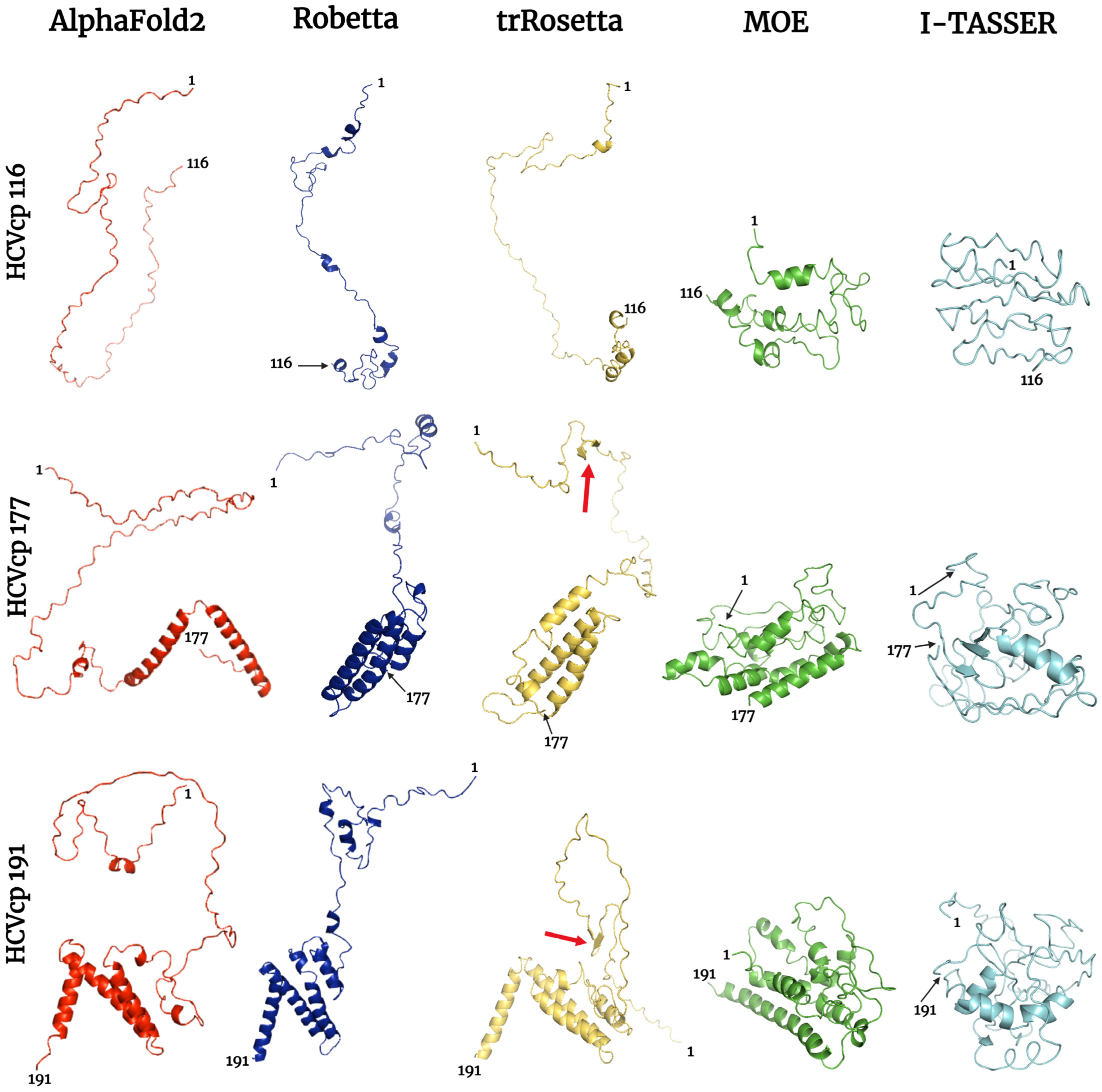
Abstract
1. Introduction
2. Materials and Methods
2.1. Amino Acid Sequence of HCVcp
2.2. Prediction of the Secondary Structures of HCVcp
2.3. Structural Modeling of HCVcp
2.4. Visualization and Analysis of the Predicted Models
2.5. MD Simulations
3. Results
3.1. HCVcp Models
3.2. Model Ranks and Structure Interpretations
3.3. Results of Stereochemical Analysis
3.4. Results of MD Simulations
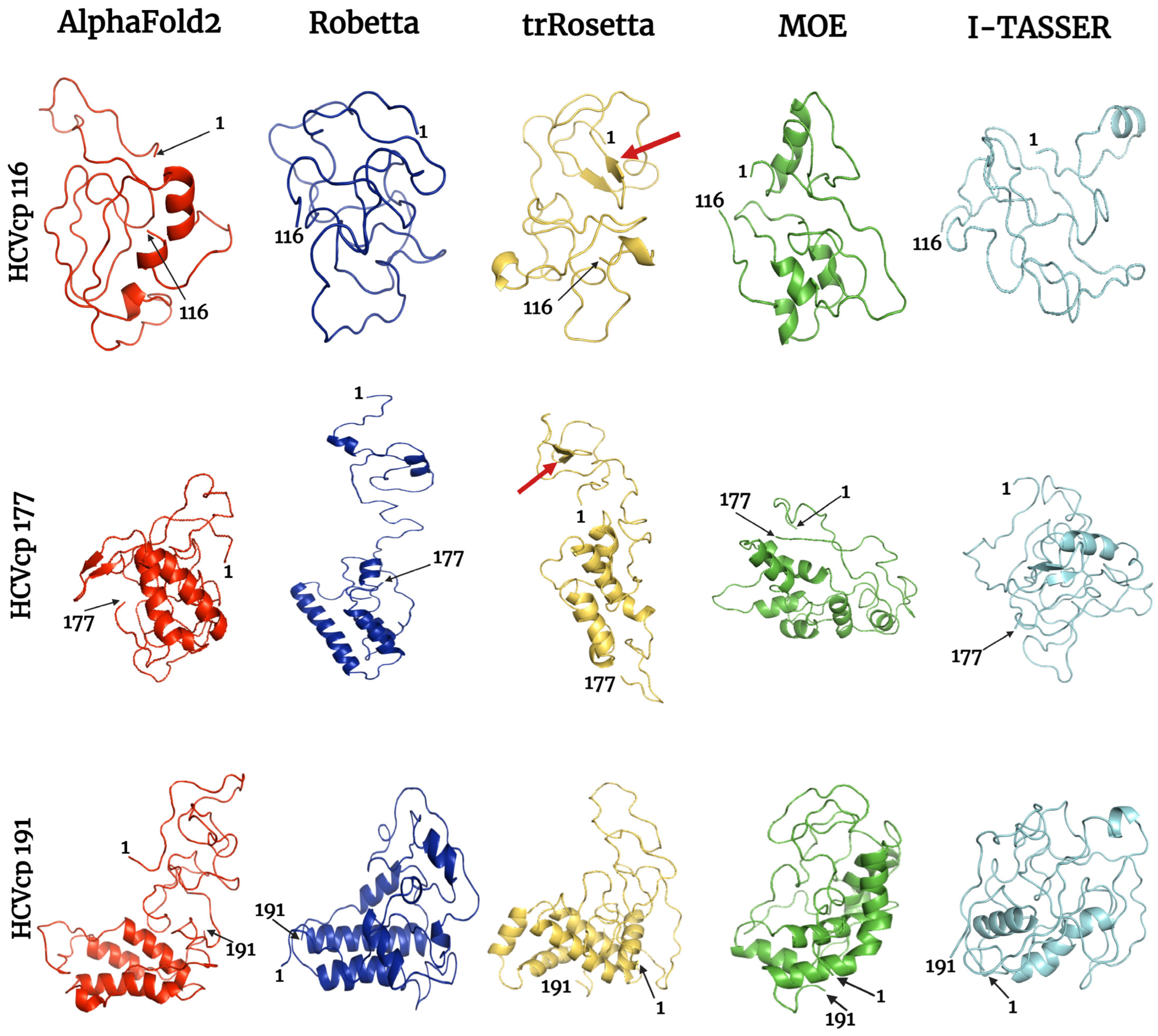
3.5. Results of Refined Structure Analysis
3.6. Results of Structural Validation
4. Discussion
Supplementary Materials
Author Contributions
Funding
Institutional Review Board Statement
Informed Consent Statement
Data Availability Statement
Acknowledgments
Conflicts of Interest
References
- Ornes, S. Researchers turn to deep learning to decode protein structures. Proc. Natl. Acad. Sci. USA 2022, 119, e2202107119. [Google Scholar] [CrossRef]
- Pakhrin, S.C.; Shrestha, B.; Adhikari, B.; Kc, D.B. Deep learning-based advances in protein structure prediction. Int. J. Mol. Sci. 2021, 22, 5553. [Google Scholar] [CrossRef] [PubMed]
- Pearce, R.; Zhang, Y. Deep learning techniques have significantly impacted protein structure prediction and protein design. Curr. Opin. Struct. Biol. 2021, 68, 194–207. [Google Scholar] [CrossRef]
- Pearce, R.; Zhang, Y. Toward the solution of the protein structure prediction problem. J. Biol. Chem. 2021, 297, 100870. [Google Scholar] [CrossRef] [PubMed]
- Cramer, P. AlphaFold2 and the future of structural biology. Nat. Struct. Mol. Biol. 2021, 28, 704–705. [Google Scholar] [CrossRef]
- Jumper, J.; Evans, R.; Pritzel, A.; Green, T.; Figurnov, M.; Ronneberger, O.; Tunyasuvunakool, K.; Bates, R.; Zidek, A.; Potapenko, A.; et al. Highly accurate protein structure prediction with AlphaFold. Nature 2021, 596, 583–589. [Google Scholar] [CrossRef] [PubMed]
- Moult, J.; Fidelis, K.; Kryshtafovych, A.; Schwede, T.; Topf, M. Critical Assessment of Techniques for Protein Structure Prediction, Fourteenth Round; CASP 14 Abstract Book; Protein Structure Prediction Center, University of California: Davis, CA, USA, 2020. [Google Scholar]
- Pereira, J.; Simpkin, A.J.; Hartmann, M.D.; Rigden, D.J.; Keegan, R.M.; Lupas, A.N. High-accuracy protein structure prediction in CASP14. Proteins 2021, 89, 1687–1699. [Google Scholar] [CrossRef]
- Elofsson, A. Progress at protein structure prediction, as seen in CASP15. Curr. Opin. Struct. Biol. 2023, 80, 102594. [Google Scholar] [CrossRef]
- Ding, Q.; Heller, B.; Capuccino, J.M.; Song, B.; Nimgaonkar, I.; Hrebikova, G.; Contreras, J.E.; Ploss, A. Hepatitis E virus ORF3 is a functional ion channel required for release of infectious particles. Proc. Natl. Acad. Sci. USA 2017, 114, 1147–1152. [Google Scholar] [CrossRef]
- Skolnick, J.; Gao, M.; Zhou, H.; Singh, S. AlphaFold 2: Why it works and its implications for understanding the relationships of protein sequence, structure, and function. J. Chem. Inf. Model 2021, 61, 4827–4831. [Google Scholar] [CrossRef]
- Baek, M.; DiMaio, F.; Anishchenko, I.; Dauparas, J.; Ovchinnikov, S.; Lee, G.R.; Wang, J.; Cong, Q.; Kinch, L.N.; Schaeffer, R.D.; et al. Accurate prediction of protein structures and interactions using a three-track neural network. Science 2021, 373, 871–876. [Google Scholar] [CrossRef] [PubMed]
- Lee, C.; Su, B.H.; Tseng, Y.J. Comparative studies of AlphaFold, RoseTTAFold and Modeller: A case study involving the use of G-protein-coupled receptors. Brief Bioinform. 2022, 23, bbac308. [Google Scholar] [CrossRef] [PubMed]
- Du, Z.; Su, H.; Wang, W.; Ye, L.; Wei, H.; Peng, Z.; Anishchenko, I.; Baker, D.; Yang, J. The trRosetta server for fast and accurate protein structure prediction. Nat. Protoc. 2021, 16, 5634–5651. [Google Scholar] [CrossRef]
- Haddad, Y.; Adam, V.; Heger, Z. Ten quick tips for homology modeling of high-resolution protein 3D structures. PLoS Comput. Biol. 2020, 16, e1007449. [Google Scholar] [CrossRef] [PubMed]
- Krieger, E.; Nabuurs, S.B.; Vriend, G. Homology modeling. Methods Biochem. Anal. 2003, 44, 509–523. [Google Scholar] [CrossRef]
- Zheng, W.; Zhang, C.; Li, Y.; Pearce, R.; Bell, E.W.; Zhang, Y. Folding non-homologous proteins by coupling deep-learning contact maps with I-TASSER assembly simulations. Cell Rep. Methods 2021, 1, 100014. [Google Scholar] [CrossRef] [PubMed]
- Yang, J.; Yan, R.; Roy, A.; Xu, D.; Poisson, J.; Zhang, Y. The I-TASSER Suite: Protein structure and function prediction. Nat. Methods 2015, 12, 7–8. [Google Scholar] [CrossRef]
- Yang, J.; Zhang, Y. I-TASSER server: New development for protein structure and function predictions. Nucleic Acids Res. 2015, 43, W174–W181. [Google Scholar] [CrossRef]
- Roy, A.; Kucukural, A.; Zhang, Y. I-TASSER: A unified platform for automated protein structure and function prediction. Nat. Protoc. 2010, 5, 725–738. [Google Scholar] [CrossRef]
- Zhang, Y. I-TASSER server for protein 3D structure prediction. BMC Bioinform. 2008, 9, 40. [Google Scholar] [CrossRef]
- Kao, C.C.; Yi, G.; Huang, H.C. The core of hepatitis C virus pathogenesis. Curr. Opin. Virol. 2016, 17, 66–73. [Google Scholar] [CrossRef]
- Moradpour, D.; Penin, F. Hepatitis C virus proteins: From structure to function. Curr. Top Microbiol. Immunol. 2013, 369, 113–142. [Google Scholar] [CrossRef] [PubMed]
- Chinnaswamy, S.; Yarbrough, I.; Palaninathan, S.; Kumar, C.T.; Vijayaraghavan, V.; Demeler, B.; Lemon, S.M.; Sacchettini, J.C.; Kao, C.C. A locking mechanism regulates RNA synthesis and host protein interaction by the hepatitis C virus polymerase. J. Biol. Chem. 2008, 283, 20535–20546. [Google Scholar] [CrossRef] [PubMed]
- Mani, H.; Chen, Y.C.; Chen, Y.K.; Liu, W.L.; Lo, S.Y.; Lin, S.H.; Liou, J.W. Nanosized particles assembled by a recombinant virus protein are able to encapsulate negatively charged molecules and structured RNA. Polymers 2021, 13, 858. [Google Scholar] [CrossRef] [PubMed]
- Mani, H.; Yen, J.H.; Hsu, H.J.; Chang, C.C.; Liou, J.W. Hepatitis C virus core protein: Not just a nucleocapsid building block, but an immunity and inflammation modulator. Tzu Chi. Med. J. 2022, 34, 139–147. [Google Scholar] [CrossRef]
- Wang, X.; Zhou, Y.; Wang, C.; Zhao, Y.; Cheng, Y.; Yu, S.; Li, X.; Zhang, W.; Zhang, Y.; Quan, H. HCV Core protein represses DKK3 expression via epigenetic silencing and activates the Wnt/beta-catenin signaling pathway during the progression of HCC. Clin. Transl. Oncol. 2022, 24, 1998–2009. [Google Scholar] [CrossRef]
- Xu, H.; Li, G.; Yue, Z.; Li, C. HCV core protein-induced upregulation of microRNA-196a promotes aberrant proliferation in hepatocellular carcinoma by targeting FOXO1. Mol. Med. Rep. 2016, 13, 5223–5229. [Google Scholar] [CrossRef]
- Rajalakshmy, A.R.; Malathi, J.; Madhavan, H.N.; Srinivasan, B.; Iyer, G.K. Hepatitis C virus core and NS3 antigens induced conjunctival inflammation via toll-like receptor-mediated signaling. Mol. Vis. 2014, 20, 1388–1397. [Google Scholar]
- Kawasaki, T.; Kawai, T. Toll-like receptor signaling pathways. Front. Immunol. 2014, 5, 461. [Google Scholar] [CrossRef]
- Strosberg, A.D.; Kota, S.; Takahashi, V.; Snyder, J.K.; Mousseau, G. Core as a novel viral target for hepatitis C drugs. Viruses 2010, 2, 1734–1751. [Google Scholar] [CrossRef]
- Fromentin, R.; Majeau, N.; Laliberte Gagne, M.E.; Boivin, A.; Duvignaud, J.B.; Leclerc, D. A method for in vitro assembly of hepatitis C virus core protein and for screening of inhibitors. Anal. Biochem. 2007, 366, 37–45. [Google Scholar] [CrossRef]
- Uversky, V.N. Intrinsically disordered proteins from A to Z. Int. J. Biochem. Cell Biol. 2011, 43, 1090–1103. [Google Scholar] [CrossRef]
- Boni, S.; Lavergne, J.P.; Boulant, S.; Cahour, A. Hepatitis C virus core protein acts as a trans-modulating factor on internal translation initiation of the viral RNA. J. Biol. Chem. 2005, 280, 17737–17748. [Google Scholar] [CrossRef] [PubMed]
- Afzal, M.S.; Alsaleh, K.; Farhat, R.; Belouzard, S.; Danneels, A.; Descamps, V.; Duverlie, G.; Wychowski, C.; Zaidi, N.; Dubuisson, J.; et al. Regulation of core expression during the hepatitis C virus life cycle. J. Gen. Virol. 2015, 96, 311–321. [Google Scholar] [CrossRef] [PubMed]
- Jhaveri, R.; Qiang, G.; Diehl, A.M. Domain 3 of hepatitis C virus core protein is sufficient for intracellular lipid accumulation. J. Infect. Dis. 2009, 200, 1781–1788. [Google Scholar] [CrossRef][Green Version]
- Jhaveri, R.; McHutchison, J.; Patel, K.; Qiang, G.; Diehl, A.M. Specific polymorphisms in hepatitis C virus genotype 3 core protein associated with intracellular lipid accumulation. J. Infect. Dis. 2008, 197, 283–291. [Google Scholar] [CrossRef]
- Yanagi, M.; Purcell, R.H.; Emerson, S.U.; Bukh, J. Transcripts from a single full-length cDNA clone of hepatitis C virus are infectious when directly transfected into the liver of a chimpanzee. Proc. Natl. Acad. Sci. USA 1997, 94, 8738–8743. [Google Scholar] [CrossRef] [PubMed]
- Jones, D.T. Protein secondary structure prediction based on position-specific scoring matrices. J. Mol. Biol. 1999, 292, 195–202. [Google Scholar] [CrossRef]
- Buchan, D.W.A.; Jones, D.T. The PSIPRED Protein Analysis Workbench: 20 years on. Nucleic Acids Res. 2019, 47, W402–W407. [Google Scholar] [CrossRef]
- Su, H.; Wang, W.; Du, Z.; Peng, Z.; Gao, S.H.; Cheng, M.M.; Yang, J. Improved protein structure prediction using a new multi-scale network and homologous templates. Adv. Sci. 2021, 8, e2102592. [Google Scholar] [CrossRef] [PubMed]
- Yang, J.; Anishchenko, I.; Park, H.; Peng, Z.; Ovchinnikov, S.; Baker, D. Improved protein structure prediction using predicted interresidue orientations. Proc. Natl. Acad. Sci. USA 2020, 117, 1496–1503. [Google Scholar] [CrossRef]
- Mount, D.W. Using the Basic Local Alignment Search Tool (BLAST). Cold Spring Harb. Protoc. 2007, 2007, pdb.top17. [Google Scholar] [CrossRef]
- Colovos, C.; Yeates, T.O. Verification of protein structures: Patterns of nonbonded atomic interactions. Protein Sci. 1993, 2, 1511–1519. [Google Scholar] [CrossRef]
- Wiederstein, M.; Sippl, M.J. ProSA-web: Interactive web service for the recognition of errors in three-dimensional structures of proteins. Nucleic Acids Res. 2007, 35, W407–W410. [Google Scholar] [CrossRef]
- Schmid, N.; Eichenberger, A.P.; Choutko, A.; Riniker, S.; Winger, M.; Mark, A.E.; van Gunsteren, W.F. Definition and testing of the GROMOS force-field versions 54A7 and 54B7. Eur. Biophys. J. 2011, 40, 843–856. [Google Scholar] [CrossRef] [PubMed]
- Chang, C.C.; Liou, J.W.; Dass, K.T.P.; Li, Y.T.; Jiang, S.J.; Pan, S.F.; Yeh, Y.C.; Hsu, H.J. Internal water channel formation in CXCR4 is crucial for G i-protein coupling upon activation by CXCL12. Commun. Chem. 2020, 3, 133. [Google Scholar] [CrossRef] [PubMed]
- Chang, C.C.; Hsu, H.J.; Yen, J.H.; Lo, S.Y.; Liou, J.W. A Sequence in the loop domain of hepatitis C virus E2 protein identified in silico as crucial for the selective binding to human CD81. PLoS ONE 2017, 12, e0177383. [Google Scholar] [CrossRef] [PubMed]
- Lin, Z.; van Gunsteren, W.F. Refinement of the application of the GROMOS 54A7 force field to beta-peptides. J. Comput. Chem. 2013, 34, 2796–2805. [Google Scholar] [CrossRef]
- Berendsen, H.J.C.; Postma, J.P.M.; Gunsteren, W.F.v.; Hermans, J. Interaction models for water in relation to protein hydration. In Intermolecular Forces; Pullman, B., Ed.; Springer: Berlin/Heidelberg, Germany, 1981; pp. 331–342. [Google Scholar] [CrossRef]
- Teleman, O.; Jonsson, B.; Engstrom, S. A molecular dynamics simulation of a water model with intramolecular degrees of freedom. Mol. Phys. 1987, 60, 193–203. [Google Scholar] [CrossRef]
- Mark, P.; Nilsson, L. Structure and dynamics of the TIP3P, SPC, and SPC/E water models at 298 K. J. Phys. Chem. A 2001, 105, 9954–9960. [Google Scholar] [CrossRef]
- GROMACS—Development-Team. Gmx Solvate. Available online: https://manual.gromacs.org/current/onlinehelp/gmx-solvate.html (accessed on 8 August 2023).
- GROMACS—Development-Team. Energy Minimization, GROMACS. Available online: https://manual.gromacs.org/current/reference-manual/algorithms/energy-minimization.html (accessed on 20 June 2023).
- Maiorov, V.N.; Crippen, G.M. Size-independent comparison of protein three-dimensional structures. Proteins 1995, 22, 273–283. [Google Scholar] [CrossRef]
- Beckstein, O.; Dotson, D.L.; Detlefs, J. Calculating Root Mean Square Quantities. Available online: https://docs.mdanalysis.org/stable/documentation_pages/analysis/rms.html (accessed on 8 August 2023).
- Mukherjee, S.; Kar, R.K.; Nanga, R.P.R.; Mroue, K.H.; Ramamoorthy, A.; Bhunia, A. Accelerated molecular dynamics simulation analysis of MSI-594 in a lipid bilayer. Phys. Chem. Chem. Phys. 2017, 19, 19289–19299. [Google Scholar] [CrossRef] [PubMed]
- Forrest, L.R.; Tang, C.L.; Honig, B. On the accuracy of homology modeling and sequence alignment methods applied to membrane proteins. Biophys. J. 2006, 91, 508–517. [Google Scholar] [CrossRef] [PubMed]
- Xiang, Z. Advances in homology protein structure modeling. Curr. Protein Pept. Sci. 2006, 7, 217–227. [Google Scholar] [CrossRef]
- Nayeem, A.; Sitkoff, D.; Krystek, S., Jr. A comparative study of available software for high-accuracy homology modeling: From sequence alignments to structural models. Protein Sci. 2006, 15, 808–824. [Google Scholar] [CrossRef]
- Bryson, K.; McGuffin, L.J.; Marsden, R.L.; Ward, J.J.; Sodhi, J.S.; Jones, D.T. Protein structure prediction servers at University College London. Nucleic Acids Res. 2005, 33, W36–W38. [Google Scholar] [CrossRef] [PubMed]
- Wang, S.; Peng, J.; Ma, J.; Xu, J. Protein secondary structure prediction using deep convolutional neural fields. Sci. Rep. 2016, 6, 18962. [Google Scholar] [CrossRef]
- McGuffin, L.J.; Bryson, K.; Jones, D.T. The PSIPRED protein structure prediction server. Bioinformatics 2000, 16, 404–405. [Google Scholar] [CrossRef]
- Boulant, S.; Vanbelle, C.; Ebel, C.; Penin, F.; Lavergne, J.P. Hepatitis C virus core protein is a dimeric alpha-helical protein exhibiting membrane protein features. J. Virol. 2005, 79, 11353–11365. [Google Scholar] [CrossRef]
- Hollingsworth, S.A.; Karplus, P.A. A fresh look at the Ramachandran plot and the occurrence of standard structures in proteins. Biomol. Concepts 2010, 1, 271–283. [Google Scholar] [CrossRef]
- Wlodawer, A. Stereochemistry and validation of macromolecular structures. Methods Mol. Biol. 2017, 1607, 595–610. [Google Scholar] [CrossRef] [PubMed]
- Sims, G.E.; Kim, S.H. A method for evaluating the structural quality of protein models by using higher-order phi-psi pairs scoring. Proc. Natl. Acad. Sci. USA 2006, 103, 4428–4432. [Google Scholar] [CrossRef] [PubMed]
- Fan, H.; Mark, A.E. Refinement of homology-based protein structures by molecular dynamics simulation techniques. Protein Sci. 2004, 13, 211–220. [Google Scholar] [CrossRef] [PubMed]
- Sippl, M.J. Recognition of errors in three-dimensional structures of proteins. Proteins 1993, 17, 355–362. [Google Scholar] [CrossRef] [PubMed]
- McPherson, A.; Gavira, J.A. Introduction to protein crystallization. Acta Crystallogr. F Struct. Biol. Commun. 2014, 70, 2–20. [Google Scholar] [CrossRef]
- Kosol, S.; Contreras-Martos, S.; Cedeno, C.; Tompa, P. Structural characterization of intrinsically disordered proteins by NMR spectroscopy. Molecules 2013, 18, 10802–10828. [Google Scholar] [CrossRef]
- Hu, Y.; Cheng, K.; He, L.; Zhang, X.; Jiang, B.; Jiang, L.; Li, C.; Wang, G.; Yang, Y.; Liu, M. NMR-based methods for protein analysis. Anal. Chem. 2021, 93, 1866–1879. [Google Scholar] [CrossRef]
- Binshtein, E.; Ohi, M.D. Cryo-electron microscopy and the amazing race to atomic resolution. Biochemistry 2015, 54, 3133–3141. [Google Scholar] [CrossRef]
- Yip, K.M.; Fischer, N.; Paknia, E.; Chari, A.; Stark, H. Atomic-resolution protein structure determination by cryo-EM. Nature 2020, 587, 157–161. [Google Scholar] [CrossRef]
- Anfinsen, C.B.; Haber, E.; Sela, M.; White, F.H., Jr. The kinetics of formation of native ribonuclease during oxidation of the reduced polypeptide chain. Proc. Natl. Acad. Sci. USA 1961, 47, 1309–1314. [Google Scholar] [CrossRef]
- Anfinsen, C.B. Principles that govern the folding of protein chains. Science 1973, 181, 223–230. [Google Scholar] [CrossRef]
- Chowdhury, R.; Bouatta, N.; Biswas, S.; Floristean, C.; Kharkar, A.; Roy, K.; Rochereau, C.; Ahdritz, G.; Zhang, J.; Church, G.M.; et al. Publisher Correction: Single-sequence protein structure prediction using a language model and deep learning. Nat. Biotechnol. 2022, 40, 1692. [Google Scholar] [CrossRef] [PubMed]
- King, R.D.; Sternberg, M.J. Identification and application of the concepts important for accurate and reliable protein secondary structure prediction. Protein Sci. 1996, 5, 2298–2310. [Google Scholar] [CrossRef] [PubMed]
- Richardson, J.S.; Richardson, D.C. Amino acid preferences for specific locations at the ends of alpha helices. Science 1988, 240, 1648–1652. [Google Scholar] [CrossRef] [PubMed]
- Lim, V.I. Algorithms for prediction of alpha-helical and beta-structural regions in globular proteins. J. Mol. Biol. 1974, 88, 873–894. [Google Scholar] [CrossRef]
- Heo, L.; Feig, M. Experimental accuracy in protein structure refinement via molecular dynamics simulations. Proc. Natl. Acad. Sci. USA 2018, 115, 13276–13281. [Google Scholar] [CrossRef]
- Azzaz, F.; Yahi, N.; Chahinian, H.; Fantini, J. The epigenetic dimension of protein structure is an intrinsic weakness of the AlphaFold program. Biomolecules 2022, 12, 1527. [Google Scholar] [CrossRef]
- Dolan, P.T.; Roth, A.P.; Xue, B.; Sun, R.; Dunker, A.K.; Uversky, V.N.; LaCount, D.J. Intrinsic disorder mediates hepatitis C virus core-host cell protein interactions. Protein Sci. 2015, 24, 221–235. [Google Scholar] [CrossRef]
- Chodera, J.D.; Noe, F. Markov state models of biomolecular conformational dynamics. Curr. Opin. Struct. Biol. 2014, 25, 135–144. [Google Scholar] [CrossRef]
- Bernardi, R.C.; Melo, M.C.R.; Schulten, K. Enhanced sampling techniques in molecular dynamics simulations of biological systems. Biochim. Biophys. Acta 2015, 1850, 872–877. [Google Scholar] [CrossRef]
- Sugita, Y.; Okamoto, Y. Replica-exchange molecular dynamics method for protein folding. Chem. Phys. Lett. 1999, 314, 141–151. [Google Scholar] [CrossRef]
- Laio, A.; Parrinello, M. Escaping free-energy minima. Proc. Natl. Acad. Sci. USA 2002, 99, 12562–12566. [Google Scholar] [CrossRef] [PubMed]


Disclaimer/Publisher’s Note: The statements, opinions and data contained in all publications are solely those of the individual author(s) and contributor(s) and not of MDPI and/or the editor(s). MDPI and/or the editor(s) disclaim responsibility for any injury to people or property resulting from any ideas, methods, instructions or products referred to in the content. |
© 2023 by the authors. Licensee MDPI, Basel, Switzerland. This article is an open access article distributed under the terms and conditions of the Creative Commons Attribution (CC BY) license (https://creativecommons.org/licenses/by/4.0/).
Share and Cite
Mani, H.; Chang, C.-C.; Hsu, H.-J.; Yang, C.-H.; Yen, J.-H.; Liou, J.-W. Comparison, Analysis, and Molecular Dynamics Simulations of Structures of a Viral Protein Modeled Using Various Computational Tools. Bioengineering 2023, 10, 1004. https://doi.org/10.3390/bioengineering10091004
Mani H, Chang C-C, Hsu H-J, Yang C-H, Yen J-H, Liou J-W. Comparison, Analysis, and Molecular Dynamics Simulations of Structures of a Viral Protein Modeled Using Various Computational Tools. Bioengineering. 2023; 10(9):1004. https://doi.org/10.3390/bioengineering10091004
Chicago/Turabian StyleMani, Hemalatha, Chun-Chun Chang, Hao-Jen Hsu, Chin-Hao Yang, Jui-Hung Yen, and Je-Wen Liou. 2023. "Comparison, Analysis, and Molecular Dynamics Simulations of Structures of a Viral Protein Modeled Using Various Computational Tools" Bioengineering 10, no. 9: 1004. https://doi.org/10.3390/bioengineering10091004
APA StyleMani, H., Chang, C.-C., Hsu, H.-J., Yang, C.-H., Yen, J.-H., & Liou, J.-W. (2023). Comparison, Analysis, and Molecular Dynamics Simulations of Structures of a Viral Protein Modeled Using Various Computational Tools. Bioengineering, 10(9), 1004. https://doi.org/10.3390/bioengineering10091004