
Deep Learning-Based Reconstruction for Cardiac MRI: A Review

 , , , , and
Abstract
1. Introduction
2. Image Reconstruction Theory
2.1. General Model
2.2. Low Rank plus Sparse Model
2.3. Partial Separability Model
3. Deep Learning-Based Reconstruction
3.1. Learning and Evaluation Procedure
3.2. Unrolled Networks
3.2.1. Neural Proximal Gradient Descent
3.2.2. Model-Based Reconstruction Using Deep-Learned Priors
3.2.3. Deep Low Rank plus Sparse
3.2.4. Deep Subspace Learning
3.3. Other Networks
4. CMR-Specific Challenges
4.1. Increased Dimensionality
4.2. Limited Training Data
5. Application-Specific Methods
5.1. Cardiovascular Blood Velocity and Flow Quantification
5.2. Late Gadolinium Enhancement
5.3. Tissue Characterization
6. Pitfalls and Future Outlook
6.1. Instabilities and Hallucinations
6.2. Interpretability
6.3. Performance Gaps
6.4. Downstream Tasks
6.5. Increased Computational Cost
6.6. Improved Models and Losses
7. Conclusions
Author Contributions
Funding
Institutional Review Board Statement
Informed Consent Statement
Data Availability Statement
Conflicts of Interest
Abbreviations
| CMR | Cardiac Magnetic Resonance |
| DL | Deep Learning |
| LV | Left Ventricle |
| MRI | Magnetic Resonance Imaging |
| L+S | Low Rank plus Sparse |
| FOV | Field of view |
| 1D | One Dimensional |
| 2D | Two Dimensional |
| 3D | Three Dimensional |
| MoDL | Model-Based Deep Learning |
| CNN | Convolutional Neural Network |
| SToRM | SmooThness Regularization on Manifolds |
| CS | Compressed Sensing |
| GPU | Graphics Processing Unit |
| NRMSE | Normalized Root Mean Squared Error |
| SSIM | Structural Similarity Index Measure |
| PSNR | Peak Signal-to-Noise Ratio |
| MSE | Mean Squared Error |
| SR | Super Resolution |
| bSSFP | Balanced Steady-State Free Precession |
| SMORE | Synthetic Multi-Orientation Resolution Enhancement |
| MEL | Memory-Efficient Learning |
| GLEAM | Greedy LEarning for Accelerated MRI |
| DIP | Deep Image Prior |
| MapNet | Mapping Network |
| TD-DIP | Time-dependent Deep Image Prior |
| PC-MRI | Phase Contrast Magnetic Resonance Imaging |
| PI | Parallel Imaging |
| LOA | Limits of Agreement |
| aAO | Ascending Aorta |
| ECG | Electrocardiogram |
| RelErr | Relative Error |
| 95%-CIs | 95 percent Confidence Intervals |
| LGE | Late Gadolinium Enhancement |
| SD | Standard Deviation |
| T1 | Longitudinal Relaxation Time |
| T2 | Transverse Relaxation Time |
| DCE | Dynamic Contrast Enhanced |
References
- Bustin, A.; Fuin, N.; Botnar, R.M.; Prieto, C. From compressed-sensing to artificial intelligence-based cardiac MRI reconstruction. Front. Cardiovasc. Med. 2020, 7, 17. [Google Scholar] [CrossRef] [PubMed]
- Ismail, T.F.; Strugnell, W.; Coletti, C.; Božić-Iven, M.; Weingärtner, S.; Hammernik, K.; Correia, T.; Küstner, T. Cardiac MR: From theory to practice. Front. Cardiovasc. Med. 2022, 9, 826283. [Google Scholar] [CrossRef] [PubMed]
- McDonagh, T.A.; Metra, M.; Adamo, M.; Gardner, R.S.; Baumbach, A.; Böhm, M.; Burri, H.; Butler, J.; Čelutkienė, J.; Chioncel, O.; et al. 2021 ESC Guidelines for the diagnosis and treatment of acute and chronic heart failure. Eur. Heart J. 2021, 42, 3599–3726. [Google Scholar] [CrossRef] [PubMed]
- Amano, Y.; Takayama, M.; Kumita, S. Contrast-enhanced myocardial T1-weighted scout (Look–Locker) imaging for the detection of myocardial damages in hypertrophic cardiomyopathy. J. Magn. Reson. 2009, 30, 778–784. [Google Scholar] [CrossRef]
- Kellman, P.; Arai, A.E.; McVeigh, E.R.; Aletras, A.H. Phase-sensitive inversion recovery for detecting myocardial infarction using gadolinium-delayed hyperenhancement. Magn. Reson. Med. 2002, 47, 372–383. [Google Scholar] [CrossRef]
- Haaf, P.; Garg, P.; Messroghli, D.R.; Broadbent, D.A.; Greenwood, J.P.; Plein, S. Cardiac T1 mapping and extracellular volume (ECV) in clinical practice: A comprehensive review. J. Cardiovasc. Magn. Reson. 2017, 18, 1–12. [Google Scholar] [CrossRef]
- Messroghli, D.R.; Radjenovic, A.; Kozerke, S.; Higgins, D.M.; Sivananthan, M.U.; Ridgway, J.P. Modified Look-Locker inversion recovery (MOLLI) for high-resolution T1 mapping of the heart. Magn. Reson. Med. 2004, 52, 141–146. [Google Scholar] [CrossRef]
- Kellman, P.; Hansen, M.S. T1-mapping in the heart: Accuracy and precision. J. Cardiovasc. Magn. Reson. 2014, 16, 1–20. [Google Scholar] [CrossRef]
- Chow, K.; Flewitt, J.A.; Green, J.D.; Pagano, J.J.; Friedrich, M.G.; Thompson, R.B. Saturation recovery single-shot acquisition (SASHA) for myocardial T1 mapping. Magn. Reson. Med. 2014, 71, 2082–2095. [Google Scholar] [CrossRef]
- Huang, T.Y.; Liu, Y.J.; Stemmer, A.; Poncelet, B.P. T2 measurement of the human myocardium using a T2-prepared transient-state TrueFISP sequence. Magn. Reson. Med. 2007, 57, 960–966. [Google Scholar] [CrossRef]
- Anderson, L.; Holden, S.; Davis, B.; Prescott, E.; Charrier, C.; Bunce, N.; Firmin, D.; Wonke, B.; Porter, J.; Walker, J.; et al. Cardiovascular T2-star (T2*) magnetic resonance for the early diagnosis of myocardial iron overload. Eur. Heart J. 2001, 22, 2171–2179. [Google Scholar] [CrossRef] [PubMed]
- Babu-Narayan, S.V.; Giannakoulas, G.; Valente, A.M.; Li, W.; Gatzoulis, M.A. Imaging of congenital heart disease in adults. Eur. Heart J. 2016, 37, 1182–1195. [Google Scholar] [CrossRef] [PubMed]
- Marelli, A.J.; Mackie, A.S.; Ionescu-Ittu, R.; Rahme, E.; Pilote, L. Congenital heart disease in the general population: Changing prevalence and age distribution. Circ 2007, 115, 163–172. [Google Scholar] [CrossRef] [PubMed]
- Ntsinjana, H.N.; Hughes, M.L.; Taylor, A.M. The role of cardiovascular magnetic resonance in pediatric congenital heart disease. J. Cardiovasc. Magn. Reson. 2011, 13, 1–20. [Google Scholar] [CrossRef] [PubMed]
- Cheng, J.Y.; Hanneman, K.; Zhang, T.; Alley, M.T.; Lai, P.; Tamir, J.I.; Uecker, M.; Pauly, J.M.; Lustig, M.; Vasanawala, S.S. Comprehensive motion-compensated highly accelerated 4D flow MRI with ferumoxytol enhancement for pediatric congenital heart disease. J. Magn. Reson. 2016, 43, 1355–1368. [Google Scholar] [CrossRef]
- Wang, Y.; Watts, R.; Mitchell, I.R.; Nguyen, T.D.; Bezanson, J.W.; Bergman, G.W.; Prince, M.R. Coronary MR angiography: Selection of acquisition window of minimal cardiac motion with electrocardiography-triggered navigator cardiac motion prescanning—Initial results. Radiology 2001, 218, 580–585. [Google Scholar] [CrossRef]
- Bluemke, D.A.; Boxerman, J.L.; Atalar, E.; McVeigh, E.R. Segmented K-space cine breath-hold cardiovascular MR imaging: Part 1. Principles and technique. AJR Am. J. Roentgenol. 1997, 169, 395. [Google Scholar] [CrossRef]
- Weiger, M.; Börnert, P.; Proksa, R.; Schäffter, T.; Haase, A. Motion-adapted gating based on k-space weighting for reduction of respiratory motion artifacts. Magn. Reson. Med. 1997, 38, 322–333. [Google Scholar] [CrossRef]
- Pruessmann, K.P.; Weiger, M.; Scheidegger, M.B.; Boesiger, P. SENSE: Sensitivity encoding for fast MRI. Magn. Reson. Med. 1999, 42, 952–962. [Google Scholar] [CrossRef]
- Griswold, M.A.; Jakob, P.M.; Heidemann, R.M.; Nittka, M.; Jellus, V.; Wang, J.; Kiefer, B.; Haase, A. Generalized autocalibrating partially parallel acquisitions (GRAPPA). Magn. Reson. Med. 2002, 47, 1202–1210. [Google Scholar] [CrossRef]
- Sodickson, D.K.; Manning, W.J. Simultaneous acquisition of spatial harmonics (SMASH): Fast imaging with radiofrequency coil arrays. Magn. Reson. Med. 1997, 38, 591–603. [Google Scholar] [CrossRef] [PubMed]
- Lustig, M.; Donoho, D.; Pauly, J.M. Sparse MRI: The application of compressed sensing for rapid MR imaging. Magn. Reson. Med. 2007, 58, 1182–1195. [Google Scholar] [CrossRef]
- Tariq, U.; Hsiao, A.; Alley, M.; Zhang, T.; Lustig, M.; Vasanawala, S.S. Venous and arterial flow quantification are equally accurate and precise with parallel imaging compressed sensing 4D phase contrast MRI. J. Magn. Reson. 2013, 37, 1419–1426. [Google Scholar] [CrossRef]
- Otazo, R.; Kim, D.; Axel, L.; Sodickson, D.K. Combination of compressed sensing and parallel imaging for highly accelerated first-pass cardiac perfusion MRI. Magn. Reson. Med. 2010, 64, 767–776. [Google Scholar] [CrossRef] [PubMed]
- Hsiao, A.; Lustig, M.; Alley, M.T.; Murphy, M.; Chan, F.P.; Herfkens, R.J.; Vasanawala, S.S. Rapid pediatric cardiac assessment of flow and ventricular volume with compressed sensing parallel imaging volumetric cine phase-contrast MRI. AJR Am. J. Roentgenol. 2012, 198, W250. [Google Scholar] [CrossRef]
- Otazo, R.; Candes, E.; Sodickson, D.K. Low-rank plus sparse matrix decomposition for accelerated dynamic MRI with separation of background and dynamic components. Magn. Reson. Med. 2015, 73, 1125–1136. [Google Scholar] [CrossRef]
- Knoll, F.; Murrell, T.; Sriram, A.; Yakubova, N.; Zbontar, J.; Rabbat, M.; Defazio, A.; Muckley, M.J.; Sodickson, D.K.; Zitnick, C.L.; et al. Advancing machine learning for MR image reconstruction with an open competition: Overview of the 2019 fastMRI challenge. Magn. Reson. Med. 2020, 84, 3054–3070. [Google Scholar] [CrossRef] [PubMed]
- Muckley, M.J.; Riemenschneider, B.; Radmanesh, A.; Kim, S.; Jeong, G.; Ko, J.; Jun, Y.; Shin, H.; Hwang, D.; Mostapha, M.; et al. Results of the 2020 fastmri challenge for machine learning mr image reconstruction. IEEE Trans. Med. Imaging 2021, 40, 2306–2317. [Google Scholar] [CrossRef] [PubMed]
- Knoll, F.; Hammernik, K.; Zhang, C.; Moeller, S.; Pock, T.; Sodickson, D.K.; Akcakaya, M. Deep-learning methods for parallel magnetic resonance imaging reconstruction: A survey of the current approaches, trends, and issues. IEEE Signal Process. Mag. 2020, 37, 128–140. [Google Scholar] [CrossRef]
- Hammernik, K.; Schlemper, J.; Qin, C.; Duan, J.; Summers, R.M.; Rueckert, D. Systematic evaluation of iterative deep neural networks for fast parallel MRI reconstruction with sensitivity-weighted coil combination. Magn. Reson. Med. 2021, 86, 1859–1872. [Google Scholar] [CrossRef]
- Donoho, D.L. Compressed sensing. IEEE Trans. Inf. Theory 2006, 52, 1289–1306. [Google Scholar] [CrossRef]
- Candès, E.J.; Romberg, J.; Tao, T. Robust uncertainty principles: Exact signal reconstruction from highly incomplete frequency information. IEEE Trans. Inf. Theory 2006, 52, 489–509. [Google Scholar] [CrossRef]
- Hammernik, K.; Klatzer, T.; Kobler, E.; Recht, M.P.; Sodickson, D.K.; Pock, T.; Knoll, F. Learning a variational network for reconstruction of accelerated MRI data. Mag. Reson. Med. 2018, 79, 3055–3071. [Google Scholar] [CrossRef] [PubMed]
- Aggarwal, H.K.; Mani, M.P.; Jacob, M. MoDL: Model-based deep learning architecture for inverse problems. IEEE Trans. Med. Imaging 2018, 38, 394–405. [Google Scholar] [CrossRef]
- Mardani, M.; Sun, Q.; Donoho, D.; Papyan, V.; Monajemi, H.; Vasanawala, S.; Pauly, J. Neural proximal gradient descent for compressive imaging. Adv. Neural. Inf. Process. Syst. 2018, 31. Available online: https://proceedings.neurips.cc/paper/2018/hash/61d009da208a34ae155420e55f97abc7-Abstract.html (accessed on 2 March 2023).
- Sandino, C.M.; Cheng, J.Y.; Chen, F.; Mardani, M.; Pauly, J.M.; Vasanawala, S.S. Compressed sensing: From research to clinical practice with deep neural networks: Shortening scan times for magnetic resonance imaging. IEEE Signal Process. Mag. 2020, 37, 117–127. [Google Scholar] [CrossRef]
- Sandino, C.M.; Lai, P.; Vasanawala, S.S.; Cheng, J.Y. Accelerating cardiac cine MRI using a deep learning-based ESPIRiT reconstruction. Magn. Reson. Med. 2021, 85, 152–167. [Google Scholar] [CrossRef]
- Zucker, E.J.; Sandino, C.M.; Kino, A.; Lai, P.; Vasanawala, S.S. Free-breathing Accelerated Cardiac MRI Using Deep Learning: Validation in Children and Young Adults. Radiology 2021, 300, 539–548. [Google Scholar] [CrossRef]
- Oscanoa, J.A.; Middione, M.J.; Syed, A.B.; Sandino, C.M.; Vasanawala, S.S.; Ennis, D.B. Accelerated two-dimensional phase-contrast for cardiovascular MRI using deep learning-based reconstruction with complex difference estimation. Mag. Reson. Med. 2023, 89, 356–369. [Google Scholar] [CrossRef] [PubMed]
- Küstner, T.; Fuin, N.; Hammernik, K.; Bustin, A.; Qi, H.; Hajhosseiny, R.; Masci, P.G.; Neji, R.; Rueckert, D.; Botnar, R.M.; et al. CINENet: Deep learning-based 3D cardiac CINE MRI reconstruction with multi-coil complex-valued 4D spatio-temporal convolutions. Sci. Rep. 2020, 10, 1–13. [Google Scholar] [CrossRef] [PubMed]
- Biswas, S.; Aggarwal, H.K.; Jacob, M. Dynamic MRI using model-based deep learning and SToRM priors: MoDL-SToRM. Magn. Reson. Med. 2019, 82, 485–494. [Google Scholar] [CrossRef] [PubMed]
- Huang, W.; Ke, Z.; Cui, Z.X.; Cheng, J.; Qiu, Z.; Jia, S.; Ying, L.; Zhu, Y.; Liang, D. Deep low-rank plus sparse network for dynamic MR imaging. Med. Image Anal. 2021, 73, 102190. [Google Scholar] [CrossRef]
- Ozturkler, B.; Sahiner, A.; Ergen, T.; Desai, A.D.; Sandino, C.M.; Vasanawala, S.; Pauly, J.M.; Mardani, M.; Pilanci, M. GLEAM: Greedy Learning for Large-Scale Accelerated MRI Reconstruction. arXiv 2022, arXiv:2207.08393. [Google Scholar]
- Wang, K.; Kellman, M.; Sandino, C.M.; Zhang, K.; Vasanawala, S.S.; Tamir, J.I.; Yu, S.X.; Lustig, M. Memory-efficient Learning for High-Dimensional MRI Reconstruction. In Proceedings of the International Conference on Medical Image Computing and Computer-Assisted Intervention, Strasbourg, France, 27 September–1 October 2021; pp. 461–470. [Google Scholar]
- Ulyanov, D.; Vedaldi, A.; Lempitsky, V. Deep image prior. In Proceedings of the IEEE Conference on Computer Vision and Pattern Recognition, Salt Lake City, UT, USA, 18 June–23 June 2018; pp. 9446–9454. [Google Scholar]
- Acar, M.; Çukur, T.; Öksüz, İ. Self-supervised dynamic mri reconstruction. In Proceedings of the Machine Learning for Medical Image Reconstruction: 4th International Workshop, MLMIR 2021, Held in Conjunction with MICCAI 2021, Strasbourg, France, 1 October 2021; pp. 35–44. [Google Scholar]
- Haldar, J.P.; Liang, Z.P. Spatiotemporal imaging with partially separable functions: A matrix recovery approach. In Proceedings of the 2010 IEEE International Symposium on Biomedical Imaging: From Nano to Macro, Rotterdam, The Netherlands, 4–17 April 2010; pp. 716–719. [Google Scholar]
- Ong, F.; Zhu, X.; Cheng, J.Y.; Johnson, K.M.; Larson, P.E.; Vasanawala, S.S.; Lustig, M. Extreme MRI: Large-scale volumetric dynamic imaging from continuous non-gated acquisitions. Magn. Reson. Med. 2020, 84, 1763–1780. [Google Scholar] [CrossRef] [PubMed]
- Sandino, C.M.; Ong, F.; Iyer, S.S.; Bush, A.; Vasanawala, S. Deep subspace learning for efficient reconstruction of spatiotemporal imaging data. In Proceedings of the NeurIPS 2021Workshop on Deep Learning and Inverse Problems, 2021. Available online: https://openreview.net/forum?id=pjeFySy4240 (accessed on 2 March 2023).
- Lustig, M.; Santos, J.M.; Donoho, D.L.; Pauly, J.M. SPARSE: High frame rate dynamic MRI exploiting spatio-temporal sparsity.In Proceedings of the 13th Annual Meeting of the International Society for Magnetic Resonance in Medicine, 2006; Volume 2420. Available online: https://citeseerx.ist.psu.edu/document?repid=rep1&type=pdf&doi=be7217aac865de3801e3f35ee13520888aad597d (accessed on 2 March 2023).
- Usman, M.; Atkinson, D.; Odille, F.; Kolbitsch, C.; Vaillant, G.; Schaeffter, T.; Batchelor, P.G.; Prieto, C. Motion corrected compressed sensing for free-breathing dynamic cardiac MRI. Magn. Reson. Med. 2013, 70, 504–516. [Google Scholar] [CrossRef] [PubMed]
- Wetzl, J.; Schmidt, M.; Pontana, F.; Longère, B.; Lugauer, F.; Maier, A.; Hornegger, J.; Forman, C. Single-breath-hold 3-D CINE imaging of the left ventricle using Cartesian sampling. Magn. Reson. Mater. Phys. 2018, 31, 19–31. [Google Scholar] [CrossRef] [PubMed]
- Caballero, J.; Price, A.N.; Rueckert, D.; Hajnal, J.V. Dictionary learning and time sparsity for dynamic MR data reconstruction. IEEE Trans. Med. Imaging 2014, 33, 979–994. [Google Scholar] [CrossRef]
- Montefusco, L.B.; Lazzaro, D.; Papi, S.; Guerrini, C. A fast compressed sensing approach to 3D MR image reconstruction. IEEE Trans. Med. Imaging 2010, 30, 1064–1075. [Google Scholar] [CrossRef]
- Chen, C.; Li, Y.; Axel, L.; Huang, J. Real time dynamic MRI by exploiting spatial and temporal sparsity. Magn. Reson. Imaging 2016, 34, 473–482. [Google Scholar] [CrossRef]
- Pedersen, H.; Kozerke, S.; Ringgaard, S.; Nehrke, K.; Kim, W.Y. k-t PCA: Temporally constrained k-t BLAST reconstruction using principal component analysis. Magn. Reson. Med. 2009, 62, 706–716. [Google Scholar] [CrossRef]
- Zhao, B.; Haldar, J.P.; Brinegar, C.; Liang, Z.P. Low rank matrix recovery for real-time cardiac MRI. In Proceedings of the 2010 IEEE International Symposium on Biomedical Imaging: From Nano to Macro, Rotterdam, The Netherlands, 14–17 April 2010; pp. 996–999. [Google Scholar]
- Goud, S.; Hu, Y.; Jacob, M. Real-time cardiac MRI using low-rank and sparsity penalties. In Proceedings of the 2010 IEEE International Symposium on Biomedical Imaging: From Nano to Macro, Rotterdam, The Netherlands, 14–17 April 2010; pp. 988–991. [Google Scholar]
- Lingala, S.G.; Hu, Y.; DiBella, E.; Jacob, M. Accelerated dynamic MRI exploiting sparsity and low-rank structure: kt SLR. IEEE Trans. Med. Imaging 2011, 30, 1042–1054. [Google Scholar] [CrossRef] [PubMed]
- Zhao, B.; Haldar, J.P.; Christodoulou, A.G.; Liang, Z.P. Image reconstruction from highly undersampled (k, t)-space data with joint partial separability and sparsity constraints. IEEE Trans. Med. Imaging 2012, 31, 1809–1820. [Google Scholar] [CrossRef] [PubMed]
- Miao, X.; Lingala, S.G.; Guo, Y.; Jao, T.; Usman, M.; Prieto, C.; Nayak, K.S. Accelerated cardiac cine MRI using locally low rank and finite difference constraints. Magn. Reson. Imaging 2016, 34, 707–714. [Google Scholar] [CrossRef] [PubMed]
- Parikh, N.; Boyd, S. Proximal algorithms. Found. Trends Opt. 2014, 1, 127–239. [Google Scholar] [CrossRef]
- Beck, A.; Teboulle, M. A fast iterative shrinkage-thresholding algorithm for linear inverse problems. SIAM J. Imaging Sci. 2009, 2, 183–202. [Google Scholar] [CrossRef]
- Boyd, S.; Parikh, N.; Chu, E.; Peleato, B.; Eckstein, J. Distributed optimization and statistical learning via the alternating direction method of multipliers. Found. Trends Mach. Learn. 2011, 3, 1–122. [Google Scholar] [CrossRef]
- Chambolle, A.; Pock, T. A first-order primal-dual algorithm for convex problems with applications to imaging. J. Math. Imaging Vis. 2011, 40, 120–145. [Google Scholar] [CrossRef]
- Geman, D.; Yang, C. Nonlinear image recovery with half-quadratic regularization. IEEE Trans. Image Process. 1995, 4, 932–946. [Google Scholar] [CrossRef]
- Liang, Z.P. Spatiotemporal imaging with partially separable functions. In Proceedings of the 2007 IEEE International Symposium on Biomedical Imaging: From Nano to Macro, Washington, DC, USA, 12–16 April 2007; pp. 988–991. [Google Scholar]
- Wang, S.; Su, Z.; Ying, L.; Peng, X.; Zhu, S.; Liang, F.; Feng, D.; Liang, D. Accelerating magnetic resonance imaging via deep learning. In Proceedings of the 2016 IEEE International Symposium on Biomedical Imaging (ISBI) (ISBI), Prague, Czech Republic, 13–16 April 2016; pp. 514–517. [Google Scholar]
- Zhu, B.; Liu, J.Z.; Cauley, S.F.; Rosen, B.R.; Rosen, M.S. Image reconstruction by domain-transform manifold learning. Nature 2018, 555, 487–492. [Google Scholar] [CrossRef]
- Yang, G.; Yu, S.; Dong, H.; Slabaugh, G.; Dragotti, P.L.; Ye, X.; Liu, F.; Arridge, S.; Keegan, J.; Guo, Y.; et al. DAGAN: Deep de-aliasing generative adversarial networks for fast compressed sensing MRI reconstruction. IEEE Trans. Med. Imaging 2017, 37, 1310–1321. [Google Scholar] [CrossRef]
- Akçakaya, M.; Moeller, S.; Weingärtner, S.; Uğurbil, K. Scan-specific robust artificial-neural-networks for k-space interpolation (RAKI) reconstruction: Database-free deep learning for fast imaging. Magn. Reson. Med. 2019, 81, 439–453. [Google Scholar] [CrossRef] [PubMed]
- Ghodrati, V.; Shao, J.; Bydder, M.; Zhou, Z.; Yin, W.; Nguyen, K.L.; Yang, Y.; Hu, P. MR image reconstruction using deep learning: Evaluation of network structure and loss functions. Quant. Imaging Med. Surg. 2019, 9, 1516. [Google Scholar] [CrossRef]
- Kingma, D.P.; Ba, J. Adam: A method for stochastic optimization. In Proceedings of the International Conference on Learning Representations, San Diego, CA, USA, 7–9 May 2015; pp. 1–15. [Google Scholar]
- Shimron, E.; Tamir, J.I.; Wang, K.; Lustig, M. Implicit data crimes: Machine learning bias arising from misuse of public data. Proc. Natl. Acad. Sci. USA 2022, 119, e2117203119. [Google Scholar] [CrossRef] [PubMed]
- Fabian, Z.; Heckel, R.; Soltanolkotabi, M. Data augmentation for deep learning based accelerated MRI reconstruction with limited data. Proc. Mach. Learn. Res. 2021, 139, 3057–3067. [Google Scholar]
- Poddar, S.; Jacob, M. Dynamic MRI using smoothness regularization on manifolds (SToRM). IEEE Trans. Med. Imaging 2015, 35, 1106–1115. [Google Scholar] [CrossRef] [PubMed]
- Sandino, C.M.; Cheng, J.Y.; Alley, M.T.; Carl, M.; Vasanawala, S.S. Accelerated abdominal 4D flow MRI using 3D golden-angle cones trajectory. In Proceedings of the Proc Ann Mtg ISMRM, Honolulu, HI, USA, 22–27 April 2017. [Google Scholar]
- Ke, Z.; Cui, Z.X.; Huang, W.; Cheng, J.; Jia, S.; Ying, L.; Zhu, Y.; Liang, D. Deep Manifold Learning for Dynamic MR Imaging. IEEE Trans. Comput. Imaging 2021, 7, 1314–1327. [Google Scholar] [CrossRef]
- Ahmad, R.; Xue, H.; Giri, S.; Ding, Y.; Craft, J.; Simonetti, O.P. Variable density incoherent spatiotemporal acquisition (VISTA) for highly accelerated cardiac MRI. Magn. Reson. Med. 2015, 74, 1266–1278. [Google Scholar] [CrossRef] [PubMed]
- Bernstein, M.A.; Fain, S.B.; Riederer, S.J. Effect of windowing and zero-filled reconstruction of MRI data on spatial resolution and acquisition strategy. J. Magn. Reson. 2001, 14, 270–280. [Google Scholar] [CrossRef]
- Ashikaga, H.; Estner, H.L.; Herzka, D.A.; Mcveigh, E.R.; Halperin, H.R. Quantitative assessment of single-image super-resolution in myocardial scar imaging. IEEE J. Transl. Eng. Health Med. 2014, 2, 1–12. [Google Scholar] [CrossRef]
- Dong, C.; Loy, C.C.; He, K.; Tang, X. Learning a deep convolutional network for image super-resolution. In Proceedings of the European Conference on Computer Vision, Zurich, Switzerland, 6–12 September 2014; pp. 184–199. [Google Scholar]
- Yang, W.; Zhang, X.; Tian, Y.; Wang, W.; Xue, J.H.; Liao, Q. Deep learning for single image super-resolution: A brief review. IEEE Trans. Multimed. 2019, 21, 3106–3121. [Google Scholar] [CrossRef]
- Wang, Z.; Chen, J.; Hoi, S.C. Deep learning for image super-resolution: A survey. IEEE Trans. Pattern Anal. Mach. Intell. 2020, 43, 3365–3387. [Google Scholar] [CrossRef] [PubMed]
- Li, Y.; Sixou, B.; Peyrin, F. A review of the deep learning methods for medical images super resolution problems. IRBM 2021, 42, 120–133. [Google Scholar] [CrossRef]
- Masutani, E.M.; Bahrami, N.; Hsiao, A. Deep learning single-frame and multiframe super-resolution for cardiac MRI. Radiology 2020, 295, 552. [Google Scholar] [CrossRef] [PubMed]
- Ronneberger, O.; Fischer, P.; Brox, T. U-net: Convolutional networks for biomedical image segmentation. In Proceedings of the International Conference on Medical Image Computing and Computer-Assisted Intervention, Munich, Germany, 5–9 October 2015; pp. 234–241. [Google Scholar]
- Basty, N.; Grau, V. Super resolution of cardiac cine MRI sequences using deep learning. In Image Analysis for Moving Organ, Breast, and Thoracic Images; Springer: Berlin/Heidelberg, Germany, 2018; pp. 23–31. [Google Scholar]
- Zhao, C.; Dewey, B.E.; Pham, D.L.; Calabresi, P.A.; Reich, D.S.; Prince, J.L. SMORE: A self-supervised anti-aliasing and super-resolution algorithm for MRI using deep learning. IEEE Trans. Med. Imaging 2020, 40, 805–817. [Google Scholar] [CrossRef] [PubMed]
- Putzky, P.; Welling, M. Invert to learn to invert. Adv. Neural. Inf. Process. Syst. 2019, 32. Available online: https://proceedings.neurips.cc/paper/2019/hash/ac1dd209cbcc5e5d1c6e28598e8cbbe8-Abstract.html (accessed on 2 March 2023).
- Kellman, M.; Zhang, K.; Markley, E.; Tamir, J.; Bostan, E.; Lustig, M.; Waller, L. Memory-efficient learning for large-scale computational imaging. IEEE Trans. Comput. Imaging 2020, 6, 1403–1414. [Google Scholar] [CrossRef]
- Yoo, J.; Jin, K.H.; Gupta, H.; Yerly, J.; Stuber, M.; Unser, M. Time-dependent deep image prior for dynamic MRI. IEEE Trans. Med. Imaging 2021, 40, 3337–3348. [Google Scholar] [CrossRef]
- Firmin, D.; Nayler, G.; Klipstein, R.; Underwood, S.; Rees, R.; Longmore, D. In vivo validation of MR velocity imaging. J. Comput. Assist. Tomogr. 1987, 11, 751–756. [Google Scholar] [CrossRef]
- Attili, A.K.; Parish, V.; Valverde, I.; Greil, G.; Baker, E.; Beerbaum, P. Cardiovascular MRI in childhood. Arch. Dis. Child. 2011, 96, 1147–1155. [Google Scholar] [CrossRef] [PubMed]
- Nayak, K.S.; Nielsen, J.F.; Bernstein, M.A.; Markl, M.; Gatehouse, P.D.; Botnar, R.M.; Saloner, D.; Lorenz, C.; Wen, H.; Hu, B.S.; et al. Cardiovascular magnetic resonance phase contrast imaging. J. Cardiovasc. Magn. Reson. 2015, 17, 71. [Google Scholar] [CrossRef]
- Markl, M.; Frydrychowicz, A.; Kozerke, S.; Hope, M.; Wieben, O. 4D Flow MRI. J. Magn. Reson. Imaging 2012, 36, 1015–1036. [Google Scholar] [CrossRef]
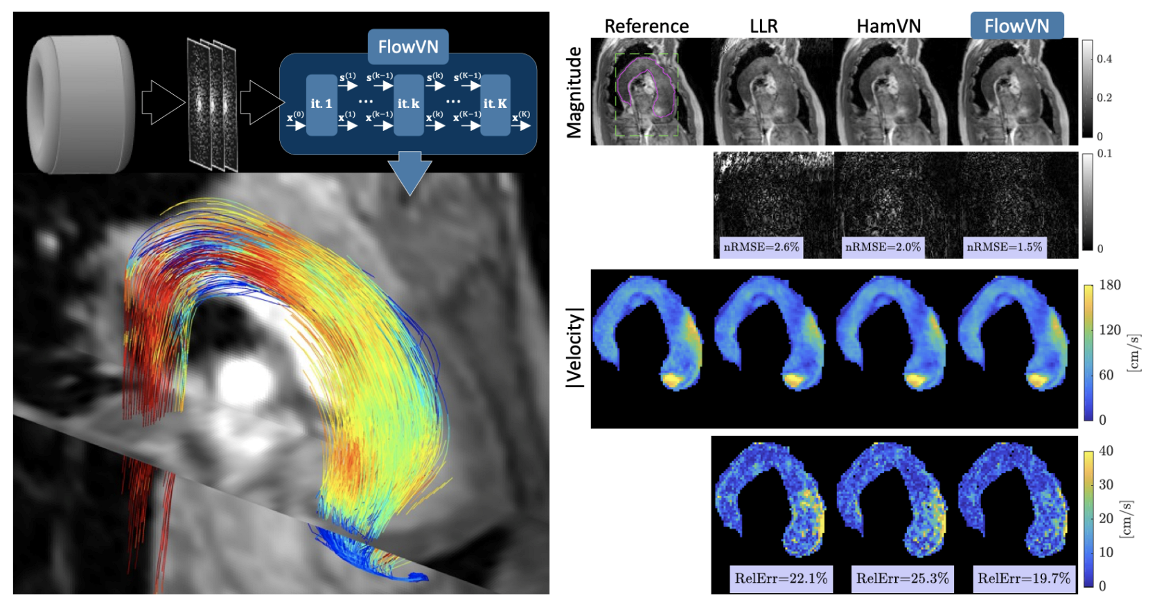
- Vishnevskiy, V.; Walheim, J.; Kozerke, S. Deep variational network for rapid 4D flow MRI reconstruction. Nat. Mach. Intell. 2020, 2, 228–235. [Google Scholar] [CrossRef]
- Haji-Valizadeh, H.; Guo, R.; Kucukseymen, S.; Paskavitz, A.; Cai, X.; Rodriguez, J.; Pierce, P.; Goddu, B.; Kim, D.; Manning, W.; et al. Highly accelerated free-breathing real-time phase contrast cardiovascular MRI via complex-difference deep learning. Mag. Reson. Med. 2021, 86, 804–819. [Google Scholar] [CrossRef] [PubMed]
- Cole, E.; Cheng, J.; Pauly, J.; Vasanawala, S. Analysis of deep complex-valued convolutional neural networks for MRI reconstruction and phase-focused applications. Mag. Reson. Med. 2021, 86, 1093–1109. [Google Scholar] [CrossRef]
- Jaubert, O.; Steeden, J.; Montalt-Tordera, J.; Arridge, S.; Kowalik, G.T.; Muthurangu, V. Deep artifact suppression for spiral real-time phase contrast cardiac magnetic resonance imaging in congenital heart disease. Mag. Reson. Med. 2021, 83, 125–132. [Google Scholar] [CrossRef]
- Jaubert, O.; Montalt-Tordera, J.; Brown, J.; Knight, D.; Arridge, S.; Steeden, J.; Muthurangu, V. FReSCO: Flow Reconstruction and Segmentation for low latency Cardiac Output monitoring using deep artifact suppression and segmentation. arXiv 2022, arXiv:2203.13729. [Google Scholar] [CrossRef] [PubMed]
- Kim, D.; Jen, M.L.; Eisenmenger, L.B.; Johnson, K.M. Accelerated 4D-flow MRI with 3-point encoding enabled by machine learning. Mag. Reson. Med. 2022, 89, 800–811. [Google Scholar] [CrossRef] [PubMed]
- Nath, R.; Callahan, S.; Stoddard, M.; Amini, A.A. FlowRAU-Net: Accelerated 4D Flow MRI of Aortic Valvular Flows with a Deep 2D Residual Attention Network. IEEE Trans. Biomed. Eng. 2022, 69, 3812–3824. [Google Scholar] [CrossRef]
- Winkelmann, S.; Schaeffter, T.; Koehler, T.; Eggers, H.; Doessel, O. An optimal radial profile order based on the Golden Ratio for time-resolved MRI. IEEE Trans. Med. Imaging 2006, 26, 68–76. [Google Scholar] [CrossRef]
- Zhang, T.; Pauly, J.M.; Levesque, I.R. Accelerating parameter mapping with a locally low rank constraint. Mag. Reson. Med. 2015, 73, 655–661. [Google Scholar] [CrossRef]
- Benkert, T.; Tian, Y.; Huang, C.; DiBella, E.V.; Chandarana, H.; Feng, L. Optimization and validation of accelerated golden-angle radial sparse MRI reconstruction with self-calibrating GRAPPA operator gridding. Mag. Reson. Med. 2018, 80, 286–293. [Google Scholar] [CrossRef]
- Kowalik, G.T.; Knight, D.; Steeden, J.A.; Muthurangu, V. Perturbed spiral real-time phase-contrast MR with compressive sensing reconstruction for assessment of flow in children. Mag. Reson. Med. 2020, 83, 2077–2091. [Google Scholar] [CrossRef] [PubMed]
- Uecker, M.; Lai, P.; Murphy, M.J.; Virtue, P.; Elad, M.; Pauly, J.M.; Vasanawala, S.S.; Lustig, M. ESPIRiT—An eigenvalue approach to autocalibrating parallel MRI: Where SENSE meets GRAPPA. Mag. Reson. Med. 2014, 71, 990–1001. [Google Scholar] [CrossRef]
- Montesinos, P.; Abascal, J.F.P.; Cussó, L.; Vaquero, J.J.; Desco, M. Application of the compressed sensing technique to self-gated cardiac cine sequences in small animals. Mag. Reson. Med. 2014, 72, 369–380. [Google Scholar] [CrossRef]
- El-Rewaidy, H.; Neisius, U.; Mancio, J.; Kucukseymen, S.; Rodriguez, J.; Paskavitz, A.; Menze, B.; Nezafat, R. Deep complex convolutional network for fast reconstruction of 3D late gadolinium enhancement cardiac MRI. NMR Biomed. 2020, 33, e4312. [Google Scholar] [CrossRef]
- Yaman, B.; Shenoy, C.; Deng, Z.; Moeller, S.; El-Rewaidy, H.; Nezafat, R.; Akçakaya, M. Self-supervised physics-guided deep learning reconstruction for high-resolution 3d lge cmr. In Proceedings of the 2021 IEEE 18th International Symposium on Biomedical Imaging (ISBI), Nice, France, 13–16 April 2021; pp. 100–104. [Google Scholar]
- van der Velde, N.; Hassing, H.C.; Bakker, B.J.; Wielopolski, P.A.; Lebel, R.M.; Janich, M.A.; Kardys, I.; Budde, R.P.; Hirsch, A. Improvement of late gadolinium enhancement image quality using a deep learning—Based reconstruction algorithm and its influence on myocardial scar quantification. Eur. Radiol. 2021, 31, 3846–3855. [Google Scholar] [CrossRef]
- Chen, Y.; Shaw, J.L.; Xie, Y.; Li, D.; Christodoulou, A.G. Deep learning within a priori temporal feature spaces for large-scale dynamic MR image reconstruction: Application to 5-D cardiac MR Multitasking. In Proceedings of the International Conference on Medical Image Computing and Computer-Assisted Intervention, Shenzhen, China, 13–17 October 2019; pp. 495–504. [Google Scholar]
- Jeelani, H.; Yang, Y.; Zhou, R.; Kramer, C.M.; Salerno, M.; Weller, D.S. A myocardial T1-mapping framework with recurrent and U-Net convolutional neural networks. In Proceedings of the 2020 IEEE International Symposium on Biomedical Imaging (ISBI), Iowa City, IA, USA, 3–7 April 2020; pp. 1941–1944. [Google Scholar]
- Hamilton, J.I.; Currey, D.; Rajagopalan, S.; Seiberlich, N. Deep learning reconstruction for cardiac magnetic resonance fingerprinting T1 and T2 mapping. Magn. Reson. Med. 2021, 85, 2127–2135. [Google Scholar] [CrossRef]
- Antun, V.; Renna, F.; Poon, C.; Adcock, B.; Hansen, A.C. On instabilities of deep learning in image reconstruction and the potential costs of AI. Proc. Natl. Acad. Sci. USA 2020, 117, 30088–30095. [Google Scholar] [CrossRef]
- Darestani, M.Z.; Chaudhari, A.S.; Heckel, R. Measuring robustness in deep learning based compressive sensing. In Proceedings of the International Conference on Machine Learning, Virtual, 18–24 July 2021; pp. 2433–2444. [Google Scholar]
- Ergen, T.; Pilanci, M. Convex duality of deep neural networks. arXiv 2020, arXiv:2002.09773. [Google Scholar]
- Pilanci, M.; Ergen, T. Neural networks are convex regularizers: Exact polynomial-time convex optimization formulations for two-layer networks. In Proceedings of the International Conference on Machine Learning, Virtual, 13–18 July 2020; pp. 7695–7705. [Google Scholar]
- Sahiner, A.; Mardani, M.; Ozturkler, B.; Pilanci, M.; Pauly, J. Convex regularization behind neural reconstruction. arXiv 2020, arXiv:2012.05169. [Google Scholar]
- Darestani, M.Z.; Liu, J.; Heckel, R. Test-Time Training Can Close the Natural Distribution Shift Performance Gap in Deep Learning Based Compressed Sensing. arXiv 2022, arXiv:2204.07204. [Google Scholar]
- Sun, L.; Fan, Z.; Ding, X.; Huang, Y.; Paisley, J. Joint CS-MRI reconstruction and segmentation with a unified deep network. In Proceedings of the International Conference on Information Processing in Medical Imaging, Hong Kong, China, 2–7 June 2019; pp. 492–504. [Google Scholar]
- Huang, Q.; Yang, D.; Yi, J.; Axel, L.; Metaxas, D. FR-Net: Joint reconstruction and segmentation in compressed sensing cardiac MRI. In Proceedings of the International Conference on Functional Imaging and Modeling of the Heart, Bordeaux, France, 6–8 June 2019; pp. 352–360. [Google Scholar]
- Gurney, P.T.; Hargreaves, B.A.; Nishimura, D.G. Design and analysis of a practical 3D cones trajectory. Magn. Reson. Med. 2006, 55, 575–582. [Google Scholar] [CrossRef] [PubMed]
- Cao, X.; Liao, C.; Iyer, S.S.; Wang, Z.; Zhou, Z.; Dai, E.; Liberman, G.; Dong, Z.; Gong, T.; He, H.; et al. Optimized multi-axis spiral projection MR fingerprinting with subspace reconstruction for rapid whole-brain high-isotropic-resolution quantitative imaging. Magn. Reson. Med. 2022, 88, 133–150. [Google Scholar] [CrossRef]
- Buehrer, M.; Pruessmann, K.P.; Boesiger, P.; Kozerke, S. Array compression for MRI with large coil arrays. Magn. Reson. Med. 2007, 57, 1131–1139. [Google Scholar] [CrossRef] [PubMed]
- Zhang, T.; Pauly, J.M.; Vasanawala, S.S.; Lustig, M. Coil compression for accelerated imaging with Cartesian sampling. Magn. Reson. Med. 2013, 69, 571–582. [Google Scholar] [CrossRef]
- Huang, F.; Vijayakumar, S.; Li, Y.; Hertel, S.; Duensing, G.R. A software channel compression technique for faster reconstruction with many channels. Magn. Reson. Imaging 2008, 26, 133–141. [Google Scholar] [CrossRef]
- Muckley, M.; Noll, D.C.; Fessler, J.A. Accelerating SENSE-type MR image reconstruction algorithms with incremental gradients. In Proceedings of the Proc Ann Mtg ISMRM, Milan, Italy, 10–16 May 2014; p. 4400. [Google Scholar]
- Pilanci, M.; Wainwright, M.J. Randomized sketches of convex programs with sharp guarantees. IEEE Trans. Inf. Theory 2015, 61, 5096–5115. [Google Scholar] [CrossRef]
- Pilanci, M.; Wainwright, M.J. Iterative Hessian sketch: Fast and accurate solution approximation for constrained least-squares. J. Mach. Learn. Res. 2016, 17, 1842–1879. [Google Scholar]
- Pilanci, M.; Wainwright, M.J. Newton sketch: A near linear-time optimization algorithm with linear-quadratic convergence. SIAM J. Optim. 2017, 27, 205–245. [Google Scholar] [CrossRef]
- Tang, J.; Golbabaee, M.; Davies, M.E. Gradient projection iterative sketch for large-scale constrained least-squares. In Proceedings of the Int Conf Mach Learn, Sydney, Australia, 6–11 August 2017; pp. 3377–3386. [Google Scholar]
- Wang, K.; Tamir, J.I.; De Goyeneche, A.; Wollner, U.; Brada, R.; Yu, S.X.; Lustig, M. High fidelity deep learning-based MRI reconstruction with instance-wise discriminative feature matching loss. Magn. Reson. Med. 2022, 88, 476–491. [Google Scholar] [CrossRef]
- Vaswani, A.; Shazeer, N.; Parmar, N.; Uszkoreit, J.; Jones, L.; Gomez, A.N.; Kaiser, Ł.; Polosukhin, I. Attention is all you need. Adv. Neural. Inf. Process. Syst. 2017, 30. Available online: https://proceedings.neurips.cc/paper/2017/hash/3f5ee243547dee91fbd053c1c4a845aa-Abstract.html (accessed on 2 March 2023).
- Dosovitskiy, A.; Beyer, L.; Kolesnikov, A.; Weissenborn, D.; Zhai, X.; Unterthiner, T.; Dehghani, M.; Minderer, M.; Heigold, G.; Gelly, S.; et al. An image is worth 16x16 words: Transformers for image recognition at scale. arXiv 2020, arXiv:2010.11929. [Google Scholar]
- Arnab, A.; Dehghani, M.; Heigold, G.; Sun, C.; Lučić, M.; Schmid, C. Vivit: A video vision transformer. In Proceedings of the IEEE/CVF International Conference on Computer Vision, Montreal, BC, Canada, 11–17 October 2021; pp. 6836–6846. [Google Scholar]
- Lin, K.; Heckel, R. Vision Transformers Enable Fast and Robust Accelerated MRI. Proc. Mach. Learn. Res. 2022, 172, 774–795. [Google Scholar]
- Korkmaz, Y.; Dar, S.U.H.; Yurt, M.; Özbey, M.; Çukur, T. Unsupervised MRI Reconstruction via Zero-Shot Learned Adversarial Transformers. IEEE Trans. Med. Imaging 2022, 41, 1747–1763. [Google Scholar] [CrossRef] [PubMed]


| Manuscript | Imaging | Network | Training | Undersampling | Recon Reduction |
|---|---|---|---|---|---|
| Vishnevskiy [97] | 4D-Flow | Unrolled | n = 11 | 12.4 ≤ R ≤ 13.8 | 30× |
| Haji-Valizadeh [98] | 2D-Flow | 3D U-Net | n = 510 | R = 28.8 | 4.6× |
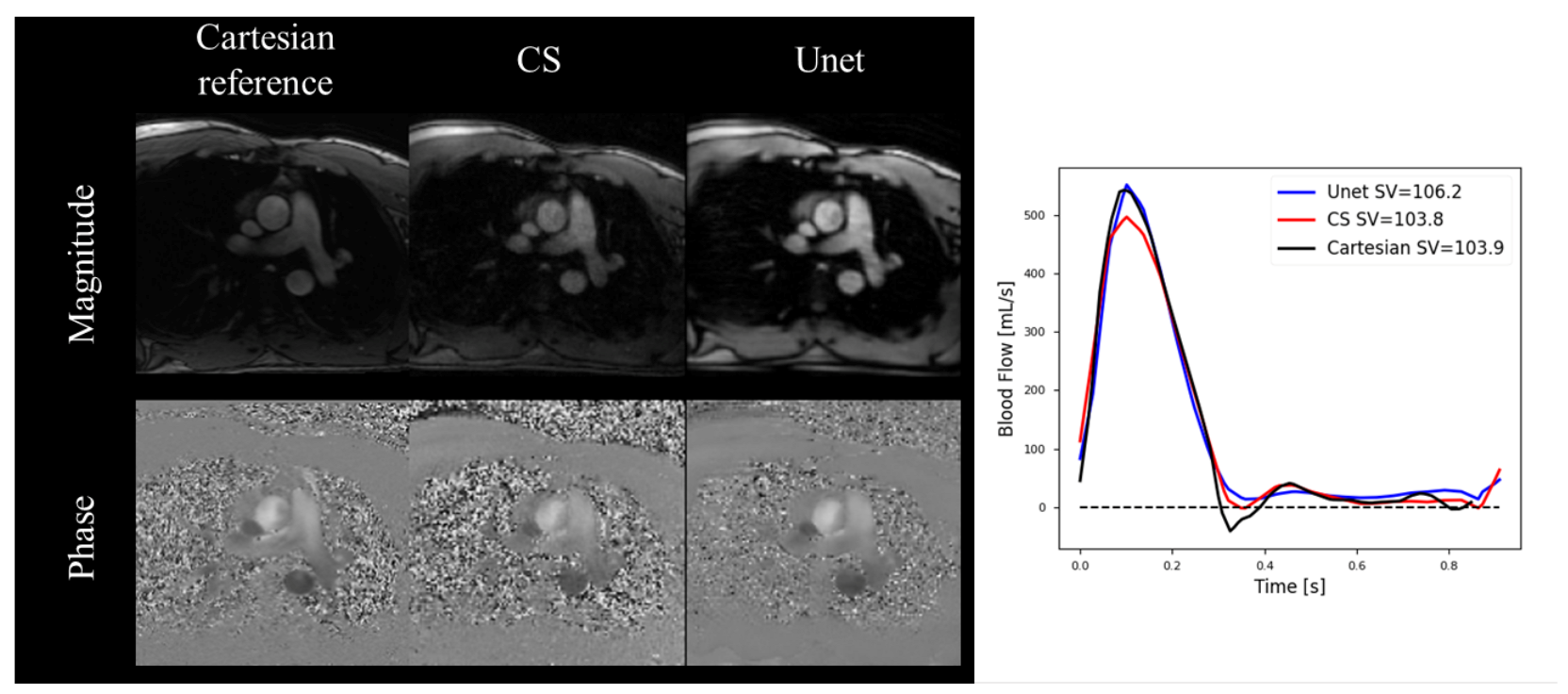
| Cole [99] | 2D-Flow | 2D U-Net | n = 180 | R ≤ 6 | N/A |
| Jaubert [100,101] | 2D-Flow | 3D U-Net | n = 520 | R = 18 | 15× |
| Oscanoa [39] | 2D-Flow | 2D U-Net | n = 155 | R = 8 | N/A |
| Kim [102] | 4D-Flow | Unrolled | n = 140 | R ≤ 6 | N/A |
| Nath [103] | 4D-Flow | 2D U-Net | n = 18 | R = 2.5, 3.3, 5 | 7× |
Disclaimer/Publisher’s Note: The statements, opinions and data contained in all publications are solely those of the individual author(s) and contributor(s) and not of MDPI and/or the editor(s). MDPI and/or the editor(s) disclaim responsibility for any injury to people or property resulting from any ideas, methods, instructions or products referred to in the content. |
© 2023 by the authors. Licensee MDPI, Basel, Switzerland. This article is an open access article distributed under the terms and conditions of the Creative Commons Attribution (CC BY) license (https://creativecommons.org/licenses/by/4.0/).
Share and Cite
Oscanoa, J.A.; Middione, M.J.; Alkan, C.; Yurt, M.; Loecher, M.; Vasanawala, S.S.; Ennis, D.B. Deep Learning-Based Reconstruction for Cardiac MRI: A Review. Bioengineering 2023, 10, 334. https://doi.org/10.3390/bioengineering10030334
Oscanoa JA, Middione MJ, Alkan C, Yurt M, Loecher M, Vasanawala SS, Ennis DB. Deep Learning-Based Reconstruction for Cardiac MRI: A Review. Bioengineering. 2023; 10(3):334. https://doi.org/10.3390/bioengineering10030334
Chicago/Turabian StyleOscanoa, Julio A., Matthew J. Middione, Cagan Alkan, Mahmut Yurt, Michael Loecher, Shreyas S. Vasanawala, and Daniel B. Ennis. 2023. "Deep Learning-Based Reconstruction for Cardiac MRI: A Review" Bioengineering 10, no. 3: 334. https://doi.org/10.3390/bioengineering10030334
APA StyleOscanoa, J. A., Middione, M. J., Alkan, C., Yurt, M., Loecher, M., Vasanawala, S. S., & Ennis, D. B. (2023). Deep Learning-Based Reconstruction for Cardiac MRI: A Review. Bioengineering, 10(3), 334. https://doi.org/10.3390/bioengineering10030334